On the rolling motion of viscous fluid on a rigid surface

Digital Commons @ NJIT

Dissertations

Theses and Dissertations

Summer 2008

On the rolling motion of viscous fluid on a rigid

surface

Xinli Wang

New Jersey Institute of Technology

Follow this and additional works at:

https://digitalcommons.njit.edu/dissertations

Part of the

Mathematics Commons

This Dissertation is brought to you for free and open access by the Theses and Dissertations at Digital Commons @ NJIT. It has been accepted for inclusion in Dissertations by an authorized administrator of Digital Commons @ NJIT. For more information, please contact

[email protected].

Recommended Citation

Wang, Xinli, "On the rolling motion of viscous fluid on a rigid surface" (2008).Dissertations. 874.

Copyright Warning & Restrictions

The copyright law of the United States (Title 17, United

States Code) governs the making of photocopies or other

reproductions of copyrighted material.

Under certain conditions specified in the law, libraries and

archives are authorized to furnish a photocopy or other

reproduction. One of these specified conditions is that the

photocopy or reproduction is not to be “used for any

purpose other than private study, scholarship, or research.”

If a, user makes a request for, or later uses, a photocopy or

reproduction for purposes in excess of “fair use” that user

may be liable for copyright infringement,

This institution reserves the right to refuse to accept a

copying order if, in its judgment, fulfillment of the order

would involve violation of copyright law.

Please Note: The author retains the copyright while the

New Jersey Institute of Technology reserves the right to

distribute this thesis or dissertation

Printing note: If you do not wish to print this page, then select

“Pages from: first page # to: last page #” on the print dialog screen

the personal information and all signatures from

the approval page and biographical sketches of

theses and dissertations in order to protect the

identity of NJIT graduates and faculty.

ON THE ROLLING MOTION OF VISCOUS FLUID ON A RIGID

SURFACE

by

Xinli Wang

This thesis considers two closely related problems. First, the influence of insoluble surfactant at a moving contact line is considered. This work is mostly motivated by the air entrainment during the coating process where there is a three-phase contact point (e.g., air, liquid and solid). For moving contact line problems, when the fluid is assumed to be an incompressible Newtonian fluid and a no-slip boundary condition is enforced at the solid boundary, the non-integrable stress singularity arises at the contact line, which is physically unrealistic. The contact angle of 180

°

is considered as a special case in which the singularity is absent. The previous work showed that there exists a non-singular local solution in the vicinity of the contact line for any capillary number. A simplified asymptotic model is used here to find a global solution with a 180

°

contact angle. Also the effects of insoluble surfactant are checked and numerical results show there exists a critical capillary number above which there is no steady state solution.

The second problem is viscous droplets rolling down a non-wettable inclined plane. The recent experiments show that the contact angle is very large (close to 180

°

) when a droplet rolls on a super-hydrophobic surface. The biharmonic boundary element method (BBEM) is used to implement numerical simulations of rolling motion. The numerical results agree well with the experimental results and theoretical prediction. Numerical evidence is also found that the stress singularity at the contact line is alleviated with a 180

°

contact angle. For droplets with insoluble surfactant on the surface, the finite volume method is used to track the evolution of

SURFACE

by Xinli Wang

A Dissertation

Submitted to the Faculty of New Jersey Institute of Technology and

Rutgers, The State University of New Jersey — Newark in Partial Fulfillment of the Requirements for the Degree of

Doctor of Philosophy in Mathematical Sciences Department of Mathematical Sciences, NJIT

Department of Mathematics and Computer Science, Rutgers-Newark August 2008

ON THE ROLLING MOTION OF VISCOUS FLUID ON A RIGID

SURFACE

Xinli Wang

Michael Siegel, Dissertation Advisor Date

Professor of Mathematics, NJIT

Michael Booty Committee Member_• Date

Associate Professor of Mathematics, NJIT

Lou Kondic, Committee Member Date

Associate Professor of Mathematics, NJIT

Charles Maldarelli, Committee Member Date

Professor of Chemical Engineering, City College of New York

Demetrios Papageorgiou, Committee Member Date

Author: Xinli Wang

Degree: Doctor of Philosophy

Date: August 2008

Undergraduate and Graduate Education: • Doctor of Philosophy in Mathematical Sciences,

New Jersey Institute of Technology, Newark, NJ, 2008 • Master of Science in Applied Mathematics,

New Jersey Institute of Technology, Newark, NJ, 2008 • Bachelor of Science in Applied Mathematics,

Shandong University, Ji'nan, Shandong, China, 2000 Major: Mathematical Sciences

I would like to thank my advisor Dr. Michael Siegel for his patient guidance and consistent encouragement. I have learned from him not only mathematical knowledge and logic way of thinking but also the optimistic and aspiring attitude to everyday life. Whenever

I

feel frustrated, he is always being there to encourage me and help me out. Without his help, this dissertation would not have been accomplished. In China, there is a saying that someone who is your teacher for one day will have been your parent for a whole lifetime. I would like to express my sincere thanks and gratitude to my advisor by this Chinese saying.

I would like to thank my committee members, Professor Demetrios Papageorgiou, Michael Booty, Lou Kondic and Charles Maldarelli for their kindness and advice in my research work. I am lucky that I have an opportunity to have them as my teachers in my Ph.D. study.

I would like to thank the Department of Mathematical Sciences for financial support during my stay at NJIT. I would also like to thank the Chinese Students and Scholars Association (CSSA) and the Office of International Students. They gave me a warm welcome as I begun my study in America.

I would like to express my gratitude to my friends Espin Leonardo and Qiming Wang for sharing experience of LATEX and MATLAB. I would like to thank my classmates Anisha Banerjee, Lakshmi Chandrasekaran and Kamyar Malakuti who gave so much help to my wife and I when our baby was born. I would also like to thank the postdoc Svetlana Tlupova who gave me some advice for numerical calculations. I wish to extend my thanks to all the friends who gave me help during my life.

My deepest appreciation goes to my family. My wife, Bin Du gave her faith, understanding, love and support to me in my life. She also brought the best gift, my lovely daughter Anna Wang to this family during my Ph.D. study. My parents's

Without love from my family, it would be impossible to achieve this.

Chapter

Page

1 INTRODUCTION

1

2 MODEL PROBLEM FOR THE CONTACT ANGLE OF H: THE FLOW

IN A CHANNEL

8

2.1 Introduction

8

2.2 Governing Equations

9

2.3 Exact Solution for No Flow

12

2.4 Asymptotic Solution

13

2.5 Exact Solution for Clean Surface

19

2.6 Numerical Results

20

3 VISCOUS DROPS ROLLING ON A SUBSTRATE

24

3.1 Introduction

24

3.2 Governing Equations

25

3.3 Biharmonic Boundary Integral Method

27

3.4 Numerical Method

32

3.5 Validation of the Code

35

3.6 Rolling Droplets

41

3.7 Numerical Analysis

55

3.8 Rolling Droplets with Surfactant

58

4 ASYMPTOTIC ANALYSIS IN THE VICINITY OF THE CONTACT LINE 64

4.1 Expansion in the Polar Coordinates

64

4.1.1 Dimensionless Equations

67

4.1.2 Previous Work for Rolling Motion

69

4.2 Lubrication Approximation at Contact Line

74

5 CONCLUSION

77

APPENDIX A CURVATURE CALCULATION BY TANGENT ANGLES .

79

(Continued)

Chapter Page

APPENDIX B CENTRAL SCHEME IN THE NON-EQUAL SPACING . . 80

APPENDIX C THE ANGLE BETWEEN THE TANGENT LINE AND THE

RADIAL LINE

82

REFERENCES

83

Figure Page

1.1

Sketch of the tape coating. The heavy line refers to a stagnant layer of

surfactant.

1

1.2

Deformation of the free surface by a vortex dipole.

3

1.3

An inviscid bubble in a two-dimensional model of Taylor's four roller mill.

4

2.1

The sketch of the flow in a channel

8

2.2

The sketch

of the contact region. A is the contact point and

S

lies on the surface. 11

2.3

Free surfaces for different values of the capillary number

22

2.4

Close-up of free surface for different values of capillary number.

22

2.5

The surfactant concentration varies as the capillary number varies

23

2.6

The solution does not exist for large Ca0. The first value of Ca0 is 0.1.

. . .

23

3.1

A schematic of a drop rolling on an inclined plane. LA is the advancing

contact angle;

R

is the receding contact angle.

25

3.2

Geometry for analytic calculation of integral on straight line segment. p

i

is a mid-point and

qj

is a node.

33

3.3

Comparison with the exact solution.

36

3.4

Evolution of a nephroid.

T1=0.2, T2=.05, T3=1, T4=1.5, T5=2, and

T6=10

36

3.5

Evolution of an ellipse. T1=0.2, T2=.05, T3=1, T4=1.5, T5=2, and T6=10. 37

3.6

Geometry of the flow in a corner. The angle of the corner is a = 1.

. . .

38

3.7

Comparison with the exact solution of the flow in a corner.The solid line

is the exact solution. The symbol "+" is the computational solution. .

39

3.8

The drop spreading driven by gravity without surface tension.T=0, T=1,

T=2, T=4, T=8, T=16, and T=32.

39

3.9

The calculation by the boundary element method shows that the steady

drop moves very slowly (velocities about 10

-3

).

* is the initial shape

and

o

is the shape at

t

= 2

41

(Continued)

Figure

Page

3.11 The steady state solution for drop spreading with gravity and surface

tension. T=0, T=1, T=2, T=4, T=8, and T=16

43

3.12 Volume conservation for a spreading drop

44

3.13 Move the contact line by a parabola through the last two grid points. .

44

3.14 Velocity field of a droplet moving on an inclined plane at

T =

1.

45

3.15 A light droplet with

ρ =

0.4 rolls on an inclined plane. Finally it reaches

a steady state. Time = 0, 1, 2, 3, 4,5, 6, 7, 8, 9, 10.

46

3.16 A light droplet with

ρ =

0.4 reaches a steady velocity.

46

3.17 A heavy droplet with

ρ =

2 rolls on the inclined plane. Finally it reaches

a steady state. Time = 0,1, 2, 3, 4,5, 6, 7, 8, 9, 10

47

3.18 A heavy droplet with

ρ =

2 reaches a steady velocity

47

3.19 The steady velocity of the rolling drop for the different liquid density. .

50

3.20 Equilibrium shape of droplets on the super-hydrophobic surface: (a) a

droplet in capillary regime; (b) a droplet in gravity regime.

0

is the

contact angle.

51

3.21 Liquid layer falls down an inclined plane.

52

3.22 Comparison of the theoretical steady velocity to numerical results for

different liquid viscosity.

53

3.23 Comparison of the theoretical steady velocity to numerical results for

different tilt angles. The angle is measured in radians

54

3.24 The footprint decreases linearly as the logarithm of the mesh size decreases

for the rolling drop with the contact angle being 120°

56

3.25 The footprint approaches slowly to a constant as the logarithm of the

mesh size decreases for the rolling drop with the contact angle being 180

°

. 56

3.26 Move the contact line by a parabola

58

3.27 Rolling drop with surfactant.

T =

0, 1, 2, 3, 4, 5, 6, 7, 8, 9, 10, 11, 12

61

3.28 A rolling drop with surfactant reaches a steady velocity.

61

3.29 Distribution of surfactant concentration at

T =

12.

62

3.30 The curvature of free surface at

T =

12.

62

(Continued)

Figure Page

3.31 The rolling motion is retarded due to the presence of surfactant.

63

4.1 The shape of free surface in the vicinity of contact line.

66

A.1 Geometry for curvature calculation. p

i

is a mid-point, and q

i

is a node.

79

B.1 Boundary elements.

80

C.1 The relationship between 0 and 9.

82

INTRODUCTION

This work is partially motivated by air entrainment in the coating of an axisymmetric or three-dimensional fiber or two dimensional tape. The coating is a covering that is applied to an object to protect it or change its physical properties. An example would be a coating applied to an optical fiber to alter its index of refraction [37].

Tape

Free Surface 1 Free Surface

Fluid velocity

Figure 1.1 Sketch of the tape coating. The heavy line refers to a stagnant layer of surfactant.

Figure 1.1 shows a schematic of tape or fiber coating. In the figure a tape is moving vertically downward into coating fluid and the speed of the tape is large enough so that the free surface deforms into a near cusp shape. Usually the tape can be coated uniformly when it is moved slowly. However, as the speed exceeds a critical value which depends on material and fluid properties, it is found that air can be entrained in the fluid in the form of tiny bubbles or long slender filaments of air that project

into the coating fluid [37]. These can ruin the coating because flaws in the form of bubbles, blemishes or voids appear in the coating on the tape or fiber surface. There has been some progress in understanding this entrainment process, but many questions remain.

Physical considerations suggest that surfactant can play an important role in the stability of the contact line and have an effect on the process of air entrainment. When surfactant is present on the free surface, the properties of the free surface change because of non-uniform distribution of surfactant (see e.g., [5,16]). This results in a surface tension gradient, the Marangoni force, which can retard the fluid motion in the vicinity of the free surface. Suppose, for example, that a given surfactant has small or zero affinity for the coating material, i.e., the tape in figure 1.1, so that it piles

up at the contact line. The accumulation of surfactant leads to a Marangoni force on the interface which opposes the downward tangential motion of the coating fluid adjacent to the free surface. When the fluid motion and interface shape are steady, and the surfactant is assumed to be insoluble and diffusion free, the Marangoni force completely retards the tangential flow at the interface, so that effectively a "no-slip" condition appears at points on the free surface where the surfactant concentration is nonzero. This is analogous to "stagnant cap" surfaces studied in [43]. Conversely, the fluid exerts a tangential force or drag on the steady interface. We hypothesize that, for sufficiently large downward tape velocity, the induced Marangoni force will not be large enough to counteract the drag on a steady state, no slip surface, and that this will lead to the nonexistence of a steady interfacial shape, and thus to an entraining flow.

There are several interesting issues related to this work. First of all, when the tape is immersed in fluid at high enough velocity, the free surface deforms into a near cusp shape near the contact line. The presence of a contact line makes mathematical modeling more complicated. A similar flow, but without complication of the contact

line, is the deformation of a free surface or inviscid bubble in a straining flow. Jeong and Moffatt [20] considered the deformation of a free surface in a two-dimensional flow acted by a vortex dipole in the figure 1.2. The undisturbed fluid occupies the

Figure 1.2 Deformation of the free surface by a vortex dipole.

half-space y < 0 and a vortex dipole of strength a is placed at z =

—di (z

is a complex variable). Jeong and Moffatt used complex analysis and conformal mapping techniques to find an exact analytical solution for the steady shapes of the free surface, which exist for all finite capillary number Ca0 = d , where is the viscosity and 'y

is the surface tension. They also found that the curvature at

P

on the free surface is proportional to e32πCa0. Thus, although the steady shape is smooth for all finite Ca 0 , it can have a very large curvature at

P,

which we refer to as a near cusp. Similar steady near cusp formation at the end of a bubble in a strain flow was found by Siegel [32]. The flow geometry considered by Siegel [32] is shown in Figure 1.3. Here a four-roller mill is filled with a highly viscous fluid and the rollers rotated in the directions shown, which produces a strain flow in the neighborhood of a bubble at the center of the mill. Exact analytical solutions were found for steady state shapes both with and without surfactant as well as for the time dependent evolution, for rather general far-field flows. In the case of certain nonlinear far-field flows produced by four rollers [2] and without surfactant, linearly stable steady state solutions exist for all capillary number defined as

Ca =

where it is the viscosity of the outer fluid,

G

is a parameter

mill.

characterizing the strain rate far from the drop,

R

is the undeformed drop radius, and 70 is the surface tension. The curvature at the end points A and

B

is exponentially

Large in the capillary number, which is similar to the Moffatt's result. When insoluble, diffusionless surfactant is present, it piles up at the end points A and

B,

and in the steady state, leads to a no-slip boundary condition near these points. The consequence Df this was found to be that there is a critical capillary number

Ca,

above which no steady solution exists. Siegel [33] also generalized the exact solution to include the time dependence, and showed that in the presence of surfactant and for

Q > Q,,

the

Free surface evolves into a transient cusp shape (i.e. with the infinite curvature). This is suggested to be related to tip-streaming [5] or entrainment. Booty and Siegel [28] studied the influence of insoluble surfactant on an inviscid axisymmetric bubble with a small aspect ratio involving in zero-Reynolds-number extensional flow. They find similar behavior, in that in absence of surfactant steady solutions exist for all

Q,

and

exist. They also derived time-dependent solutions of asymptotic equations for

Q >

Q

c

,

which exhibited the tip-streaming behavior, which is analogous to air entrainment

in the coating problem. These all motivate us to consider effect of surfactant on coating flow as shown in Figure 1.1.

What we are interested is how the contact line moves on a solid substrate if the no-slip boundary condition is enforced between the fluid and the solid substrate including at the contact line. The fluid is assumed incompressible and Newtonian. When this fluid displaces another immiscible fluid across a rigid solid, a nonintegrable stress singularity arises at the contact line [6], which is physically unrealistic. From a mathematical point of view, this singularity of the model comes from the velocity discontinuity at the contact line where, in the reference frame moving with the substrate, the solid substrate is at rest but the fluid near the contact line has to move. There are several proposed ways to remove this singularity. The one most commonly applied is to relax the no slip boundary condition [9, 26]. Another way which has received much less attention is to set the contact angle to 71 [11,25]. In view

of the importance of a nearly cusped interface morphology prior to air-entrainment in coating flows, as depicted in Figure 1.1, we are interested in this second way, i.e., setting the contact angle to 7r. Benny

&

Timson [11] (with a sign error corrected

by Dussan [7]) and Mahadevan & Pomeau [25] showed that there exists non-singular local solution in the vicinity of the contact line for any capillary number. When surfactant is present at the fluid interface, we suspect that there is a critical capillary above which steady shapes no longer exist.

The rest of work is organized as follows. In chapter 2, we consider a simplified problem involving rolling motion of a viscous fluid onto a rigid surface to analyze the influence of surfactant on an air entrainment during coating processes. In chapter 3, we consider a viscous drop rolling down an inclined non-wettable plane. The boundary element method is applied to numerically study this problem. There have

been a number of numerical studies of drops and films moving down an inclined solid substrate. Most of them studied thin drops by the lubrication approximation. Clay and Miksis [34] used a lubrication approximation to study effects of insoluble surfactant on droplet spreading. They found that surfactant can increase the speed of the translation of thin droplets. In the absence of surfactant, Homsy and his coworkers

[1] numerically studied a gravity driven two-dimensional viscous flow with a moving contact line by a boundary element method. The stress singularity at the contact line is regularized by a numerical slip boundary condition (i.e., effective slip due to the numerical discretization). Since the effective regularization or slip depends on the numerical grid spacing, the method [1] does not converge as the mesh spacing near the contact line decreases. In particular, they found in [1] that the maximum height of the profile increases linearly as the logarithm of the mesh size decreases. Zhang, Miksis, and Bankoff [18] considered the dynamics of a viscous drop moving along a substrate under the influence of shear flow in a parallel-walled channel by using the front-tracking numerical method. The no-slip condition at the bottom wall is relaxed by using a Navier-slip law so that the non-integrable stress singularity at the contact line is regularized. They showed that for small Reynolds and capillary number, steady state solutions are obtained; for large values of the parameters, the drop surface appears to rupture. However none of these has considered full numerical simulation of rolling drops with contact angles at or near 7r, and none have considered the influence of surfactant on such drop motion. Our particular interest is in developing numerical methods for nonwetting rolling drops where the stress singularity is removed by setting the contact angle to 7r. We compare our numerical results to the theoretical predictions by [25]. Chapter 4 gives the detail of a local analysis in the vicinity of the contact line with a contact angle of 180

°

. We found a mistake in Mahadevan

&

Pomeau's analysis [25]. The stream function in their analysis does not satisfy the Stokes equation if the leading order pressure is taken to be constant. However a local

parabolic shape in their analysis is consistent with the lubrication approximation

which is conveniently applied in the numerical calculation. Benney

&

Timson [11]

found a local non-singular solution for any capillary number. But the local shape

is determined by the capillary number that makes it difficulty to be applied in the

numerical calculation.

MODEL PROBLEM FOR THE CONTACT ANGLE OF

H:

THE FLOW

IN A CHANNEL

2.1 Introduction

Entrapment of air bubbles during liquid-film coating can lead to flaws such as blemishes or voids. Recent experimental studies [37] suggest there is a connection between air entrainment in coating flows and tip streaming [5] - a phenomenon well known in emulsification technology in which interfacial contaminants (surfactants) can play an important role. This motivates us to examine, via simplified mathematical models, the influence of surfactant on air entrapment during coating processes.

U

Figure 2.1

The sketch of the flow in a channel.

We consider the Stokes flow in a channel with boundaries moving at speed U (Figure 2.1). A fluid is assumed to eject from a source point 0 and be bounded by the moving boundaries and free surfaces, and insoluble surfactant is present at the interface. The distance between two boundaries is b, and the length from the source point 0 to the contact line where the fluid first meets the boundary is L. The outside region could be air or vacuum. The height of the free surface from the axis (dash line) is h(x). We assume the flux of flow is constant. The contact angle at the contact line

is assumed to be 7 which means the free surface is tangent to the solid substrate. The

contact angle at the source point 0 could be any angle. The origin of the Cartesian coordinates is at the source point 0, and the x-axes is on the axis (dash line).

2.2 Governing Equations

The fluid considered here has a large viscosity it, so the flow motion is governed by the Stokes equations

where p is the pressure and u and v are x and y components of fluid velocity respectively.

Then we consider the boundary conditions at the free surface. First we introduce the notation

[f]¹2= (f)

1

—(f)

2 that is used to describe the jump in quantities between region 1 and 2 that are separated by the interface. The fluids in the region 1 and 2 may be two different fluids (or a fluid and a hydrodynamically passive region, e.g., air). In this problem, region 1 is vacuum and region 2 is occupied by fluid. The tangential stress is balanced by the Marangoni force because of non-uniform distribution of surfactant at the interface and the normal stress is balanced by the surface tension. The tangential stress balance (TSB) is:

and the normal stress balance (NSB) is:

where 7- '/, is a unit normal vector pointing into region 1, t is a unit tangential vector,

positive for convex shapes, V3 = 7 — -->n

Fri

• 7) is the surface gradient operator [40],

and

a

is surface tension which depends on surfactant concentration F. In the two dimensional (2D) case,

Then the value at the right hand side in the equations (2.2) is

We assume a dilute concentration of surfactant, and employ a simple linear relationship between

a

and F as the equation of state, i.e.,

where σ0 is the surface tension of the clean surface, I', is the concentration of surfactant

at the contact point,

R

is the universal gas constant, and

T

is the absolute temperature. The surfactant is considered to be insoluble, or confined to the air-fluid interface for which the steady-state equation in 2D is

where u3 is the surface velocity,

D

s is the surface diffusivity which is considered to be a constant on the fluid-air interface, and subindex

s

of F and a refers to the derivative with respect to arc length

s

along the interface. Equation (2.8) is assumed to hold at the wall as well, but with a different value of

D,

than at the interface. If we consider e = -I: << 1 , to the leading order the above equation (2.8) is equivalent to

(2.4)

(2.5)

a

x

(uΓ)

=

DsΓxx,

(2.9)

where u is the x-component of the surface velocity.

At the contact point A, it is assumed that surfactant advects onto the solid boundary only from the free surface since the surfactant is considered to be insoluble i.e. there is no net flux of surfactant to and from the interface from the bulk flow. We assume the relative affinity of the surfactant for the boundary depends only on material properties of the surfactant and wall, e.g., not on velocity. At steady state, surfactant boundary condition at the contact point can be derived by integrating the equation (2.9) between a point

S

on the interface and the contact point A on the wall

Figure 2.2

The sketch of the contact region. A is the contact point and

S

lies on the

surface.

where D

s

(A) is the diffusivity

of the solid boundary which is assumed to be 0. It is

further assumed that a certain proportion A of surfactant accumulating at the contact point A streams onto the solid boundary, which means u(A)Γ(A) = UΛΓc where

U

is the velocity of the moving boundary and

F

is the surfactant concentration at the

contact point. The parameter A does not depend on the velocity and surfactant concentration at the contact line. It only depends on the material properties of the solid boundary. Then putting these two conditions into the above equation (2.11), finally we obtain the governing equation for the steady surfactant distribution at

x = S:

u(S)F(S) — UΛΓc = DsΓx(S). (2.12)

2.3 Exact Solution for No Flow If the interface shape satisfies

then lubrication theory can be applied to simplify the governing equations. We find the condition under which (2.13) holds by first seeking an exact solution in the case of no flow, i.e., both the inside fluid and the boundaries do not move. Because the flow is at rest, the pressure inside the fluid is constant (called hydrostatic pressure) and the fluid velocities are zero. In this case, the Stokes equations and the tangent stress balance equation are automatically satisfied. The normal stress balance is

—σhxx = P0,(2.14)

where a is surface tension, h(x) is the equation of free surface, and P0 is the constant

hydrostatic pressure. The boundary conditions are

Solving the second order ordinary differential equation (2.14) with boundary conditions (2.15), we get the equation of the free surface:

At the contact point

x = L,

we require the contact angle be 7 which means

h' (L)

0. This condition gives a restriction on the hydrostatic pressure:

We then use the following characteristic values to non-dimensionalize equation (2.2)

After non-dimensionalizing and dropping primes, we get the exact solution of free surface with the contact angle of 7:

Note that if the hydrostatic pressure P0 satisfies the equation (2.17) with E = Tb << 1, then the interface shape will be long and slender, and lubrication theory can

be applied to simplify the governing equations. This is done below to compute the steady interface shape when the surface is coated with insoluble surfactant and the walls move with a constant speed

U.

2.4 Asymptotic Solution

where

L

is the length from the outlet to the contact point,

U

is the velocity of the moving boundaries, and σ0 is the constant surface tension at a clean or surfactant-free interface and F, is a representative surfactant concentration. For the numerical computation of section 2.6, it is convenient to take

Γ,

equal to the surfactant concentration at the contact point between the interface and the moving walls. In this way, the surface tension equation (2.7) becomes

a =

1 — ßΓ where 3 =

Rio .

After plugging all these characteristic values into the equations and dropping the primes, we obtain the following governing equations. The Stokes equations and incompressibility condition become

where

Ca

= μ

U

is the capillary number._σ0

at the interface y = h(x) (only the upper interface is considered, the lower interface shape follows from symmetry).

From (2.12), the dimensionless steady-state equation for the surfactant concentration is found to be

(2.22)

where Pe = La' - is the Peclet number and cis evaluated on y = h(x)._AD.,

In order to keep the influence of pressure and surfactant at leading order, we rescale

(2.23)

Thus the leading order systems are: Governing equations:

(2.24a)

(2.24b)

(2.24c)

Boundary conditions are

(2.25)

( 2 . 2 6 )

The dimensionless steady state equation for surfactant is :

Next we are going to solve the leading order system and find the free surface shape y =

h(x).

Starting with the equation (2.24b), we find out that the pressure p

is the function of x and does not depend on y. Then integrate the equation (2.24a) twice with respect to y, and obtain

where

A(x)

and

B(x)

are the functions of integration. According to the symmetry

about y-axis,

A(x)

is 0. Thus

The constant

B(x)

will be determined by the flux conservation. Assume the flux to

b

e q, i.e.,

which leads to

Then the velocity u at the interface will be

From NSB equation (2.26), we get

p

x

= —h

xxx

,

then

Comparing the equation (2.25) with the equation (2.35), we obtain

(2.36)

(2.37) Integrating the above equation (2.36), we obtain

where C1 is a constant of integration. If we know the condition of hxx at the contact

point, then we will be able to determine C1. Since we assume the contact angle to

be 71, then

h

x

(L)

= 0. A summary of the boundary conditions at the contact point is

given below:

Inserting u from equation (2.34),

Γ

from equation (2.37), and F, from (2.36) into the equation (2.27), we finally obtain the governing equation for the free surface,

which can be written in the form of

The boundary conditions for this third order ODE are

The contact angle h'(0) at the outlet x =

0

is determined from the solution of the boundary value problem (2.41) and (2.42), as is the outlet surfactant concentration F(0).

Before the shooting method is applied to solve this problem numerically, we should notice that the flux constant q can be determined. In order to solve the flux q, we first consider the equation (2.40) at the contact point A where u = —1/3Ca0 hxxxh²+

hhxx-hx /2-C1 =

-1_²h - = 1 and

F =

1, thus

130

(2.43)

2.5 Exact Solution for Clean Surface

Here we consider a related special case of flow without surfactant. From the previous analysis, we know the leading order governing equations

The tangential stress balance is

and the normal stress balance is

The velocity is same as that solved for flow with surfactant. The velocity equation (2.29) is

Then the derivative of the velocity u with respect to y is

According to the tangential stress balance - no shear, we know

Thus the shape of free surface is

This is the same shape as for no flow. The reason is that all normal stress balance caring about is the hydrostatic pressure.

2.6 Numerical Results

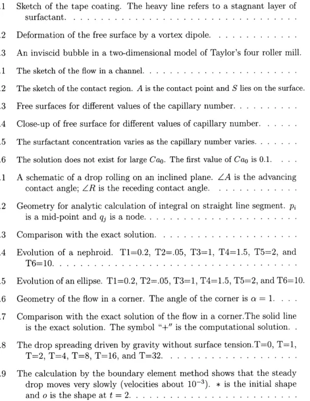
The effects of insoluble surfactant are examined numerically for the steady state motion. As the capillary number Ca0 decreases, we can consider that the characteristic velocity

U

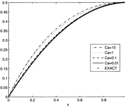
decreases, and the solution will approach the exact solution for no flow or for flow without surfactant. The Figure 2.3 shows different surface shapes for different values of Capillary number Ca 0 , and the Figure 2.4 is the close-up of the left one. The dash-dot line represents the free surface for Ca0 = 10; the dot line represents the free surface for Ca0 = 1; the dash line represents the free surface for Ca0 = 0.1; the solid line represents the free surface for Ca0 = 0.01; the empty circles represent the exact solution of free surface without flow. This numerical calculation in Figure 2.3 show exactly what we anticipated that the solid line (free surface for small Capillary number Ca0 = 0.01) approaches the exact solution of free surface without flow.

Figure 2.5 shows that surfactant concentration is more uniform when the capillary number is small than that of a large capillary number. In Figure 2.5 the dash-dot line represents surfactant concentration at interface for Ca 0 = 10; the dot line represents surfactant concentration at interface for Ca 0 = 1; the dash line represents surfactant concentration at interface for Ca 0 = 0.1; the solid line represents surfactant concentration at interface for Ca0 = 0.01. People usually use Peclet number

Pe

(the ratio of convection to diffusion along the interface) to examine the effects of surfactant. Here we use Capillary number Ca 0 to examine the effects of surfactant, which in fact is equivalent to use Peclet number because the large Capillary number means strong convention along the interface. In Figure 2.5, the solid line (for the small Capillary number Ca0 = 0.01) means when the convection along the interface is weak, the surfactant concentration is almost uniform. The dash-dot line (for the relatively large Capillary number Ca0 = 10) means when the convection along the interface is relatively large, the amount of surfactant at

x =

1 (at the contact line) is much larger than the amount of surfactant at

x =

0 (at the outlet).

In Figure 2.5, empty circles at

x =

0 represent the amount of surfactant at the outlet. We can see that the surfactant concentration at the outlet decreases as the capillary number increases. Finally the surfactant concentration is negative as the capillary number is very large in Figure 2.6 where we plot surfactant concentration at the outlet versus values of Capillary number Ca 0 . This is physically unrealistic, which means there is no steady state solution. Thus there is a critical value for capillary number above which the steady state solution does not exist.

Figure 2.3

Free surfaces for different values of the capillary number.

Figure 2.5

The surfactant concentration varies as the capillary number varies.

VISCOUS DROPS ROLLING ON A SUBSTRATE

3.1 Introduction

We consider the motion of viscus droplets on an inclined non-wettable plane which is a free surface problem with a moving contact line. Some researchers [9,25] suggest that this movement has the form of a rolling or tank-treading motion instead of a sliding motion. Recent improvements in the fabrication of extremely rough surfaces have let to the creation of super-hydrophobic surfaces. Experiments show that a drop resting on a super-hydrophobic surface has a very large contact angle (near

1800). In the natural world, there are some plant leaves having super-hydrophobic

properties [4, 45], such as lotus or water lily. Water droplets rolling on these leaves can carry away contaminating particles completely, resulting in a cleaned surface. It is called self-cleaning ability. Sliding water droplets are not effective at cleaning a surface. This self-cleaning effect is potentially useful in practical applications [27] such as waterproofing of clothes, anti-rain windshields and materials of very low friction in water,

etc.

David Quere and collaborators [8, 36] did some experiments

of viscous drops rolling on an inclined non-wettable solid and showed some very interesting properties of rolling droplets in two different regimes: (a) capillary force is dominant when the drop size is less than capillary length (σ/pg)¹/² ; (

b)

the gravity is

dominant when the drop size is larger than the capillary length (L)1/2 (where

a

is

surface tension,

p

is liquid density and

g

is acceleration of gravity). Mahadevan and Pomeau [25] gave a theoretical prediction of the steady drop velocity by using a rough scaling analysis. We are interested in performing numerical computations to verify the conclusions of Mahadeven and Pomeaus scaling theory by using the boundary element method.

3.2 Governing Equations

Consider a region Q of fluid separated by a surface

O

from an inviscid or passive fluid. The fluid may also be in contact with a solid boundary as shown in Figure 3.1.

Figure 3.1 A schematic of a drop rolling on an inclined plane. LA is the advancing contact angle;

R

is the receding contact angle.

We assume the dynamics inside the drop is governed by the Stokes equations:

where u(x, y) is the fluid velocity, p(x , y) is the pressure, p is the density (assumed constant), u is the viscosity and g is the acceleration of gravity.

On the free boundary separating Q from passive fluid, there are three boundary conditions: kinematic condition; normal stress balance; tangential stress balance. The kinematic condition means fluid particles stay on the surface. The velocity (ux, uy) of

which satisfies

and aΩ is the boundary. The stress balance conditions at the free surface are

where _Tip is stress tensor

(3.6)

ni is outward normal unit vector (i.e. pointed into the inviscid fluid), ti is the tangent

unit vector oriented counter-clockwise, σ(Γ)) is the surface tension depending on the surfactant concentration and ic is the curvature of the surface which is defined to be positive for convex surfaces. It is assumed without loss of generality that the constant pressure outside the drop is zero. On the other hand, these stress balance conditions can be written in the form:

Tangential Stress Balance (TSB):

(3.7)

Normal Stress Balance (NSB):

where un and lit are the normal and tangential components of the velocity, and σ(Γ)

The governing equation for the surfactant concentration is a convection-diffusion equation [17]:

where

t

is time, vs = v —n(n•v) is the surface gradient [40], us is the velocity vector

tangent to the interface,

X(s, t)

is a parametric representation of the interface, and

D,

is the surface diffusivity. Here we have considered the surfactant to be insoluble, i.e., there is no net flux of surfactant to and from the interface from the bulk liquid.

At the no-slip surface, the velocity of the fluid is equal to the velocity of the solid wall:

3.3 Biharmonic Boundary Integral Method

There is a large body of literature on the biharmonic boundary integral method ( [15], [29], [30], [38], [39], [41]) solving free surface viscous flow problems. This method enables us to reformulate the original differential equations which hold on the entire fluid domain as integral equations on only the domain boundary. Thus we only need to discretize the boundary rather than the entire domain. This results in a significant reduction in computational effort. In the plane flow, we introduce the streamfunction W and the vorticity w.

Here we define the vorticity to be the negative curl of velocity. Then the Stokes equations can be written in the well-known form of:

By using the biharmonic boundary integral method, equations (3.13) and (3.14) can be rewritten as a coupled set of integral equations involving the streamfunction, vorticity, and their normal derivatives on the domain boundary ( [29], [30]).

where

2. 50(q)

refers to the differential increment of

aΩ

at

q.

3. G1 and G2 are given by

and are the fundamental solutions to

where

9

is the internal angle included between the tangents to aΩ on either side of p. If the boundary aΩ is smooth, then

9

= 7r. The angle

9

can take on other values at a three phase contact point where the free surface does not always smoothly connect with the solid substrate.

Now the governing equations only depend on the stream function, vorticity, and their normal derivatives. In order to define our problem in such a way that the whole system only depends on the four variables ψ, w and 19:91,-;,), we have to write the

boundary conditions in terms of these quantities. Here we follow the derivation of the desired boundary equations from Betula [41] and Kuiken [15]. We first consider the tangential stress balance at the free surface. Substituting the following equations

into the tangential stress balance equation (3.7), we have

which holds on the boundary as In addition, the vorticity at the contour is

We eliminate the second derivative with respect to the normal direction 0- using equation (3.21) to get the tangential stress balance condition,

Secondly, we consider the normal stress balance at the free surface. Substituting the normal velocity in terms of the streamfunction into the normal stress balance equation (3.8), we get

where the pressure p is unknown. We use the governing Stokes equation to eliminate p. First differentiate the above equation (3.24) with respect to the tangential direction,

On the other hand, the tangential component of the governing equation is,

where the unit tangent vector is (tx, t

y

) and the tilt angle is a. The term (tx sin a — t

y

cos a) is the dot product of the gravity vector and the tangent vector. It appears here because the coordinate system is set up in such a way that x axis is parallel to the plane surface and y axis is perpendicular to the plane surface, and then the unit direction of the gravity vector is (sin a, — cos a). Comparing the above two equations (3.25) and (3.26) and eliminating

at

we obtain

It will be convenient in the numerical calculation to express the derivatives with respect to the tangent direction in terms of derivatives with respect to the contour

Then the tangential stress balance condition (3.23) is

The normal stress balance condition (3.27) is

Third, we consider the kinematic boundary condition through which we will determine how the fluid surface moves in time:

Finally, we describe the boundary condition at the interface between a solid wall and the fluid. Here we use the no-slip condition which means the velocity of fluid is equal to the velocity of the solid wall.

In all our calculations, the wall is rest Uwall = 0 where _Uwall indicates the velocity of

the wall, which means:

3.4 Numerical Method

We discretize the boundary polygonally into an N-gon and approximate the flow variables as being constant over each line of the N-gon. Here we consider all unknown values at the mid-points so that we can avoid calculating the flow values at the contact line. Then the governing equation can be written as the summations:

(3.34)

(3.35)

where the flow variables ‘113 (4)2 and 19

.

`"). are unknown variables, and the integrals

of Green's functions and their derivatives can be evaluated analytically as discussed later. Then these two equations can be written in the form of matrix equations,

(3.36) (3.37)

where A,

B, C

and

D

are matrices, and , w and

an

are vectors [29, 30]. The

elements of the matrices are

(3.38) (3.39) (3.40) (3.41)

where δij is the Kronecker delta, i.e., δij = 1 if i = j, otherwise δij = 0. All these

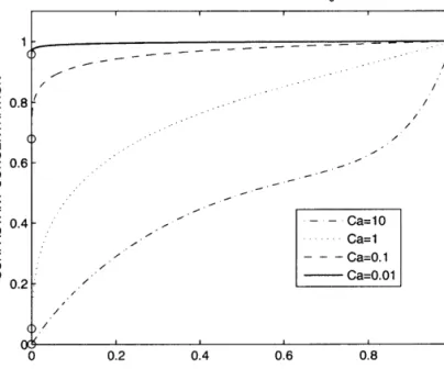
elements can be calculated analytically. We first define the following values in Figure 3.2:

h

Figure 3.2

Geometry for analytic calculation of integral on straight line segment. pi is a mid-point and qj is a node.

discretization and 2N equations. The other 2N equations come from the normal and tangential stress balance conditions. The general centered second-order discretized derivative operators (see Appendix B) are used for these two equations. We write them in the form of matrix:

where

R, S, T, U, V

and W are

N x N

matrices. At the free surface, we have

R

is a tridiagonal matrix, Sid = 0, Tip = —(Sid, V is a tridiagonal matrix as well and

Wig -=

b

is a vector containing the force of surface tension and the gravity. At

the no-slip interface, assuming Uwall = 0, we have

R

id = 1 Vij = 1, _Si.? 0, Tip = 0, Uij = 0, and bi = 0.

For a given initial shape, we can solve the following vector system by an LU decomposition.

After solving the values of the stream function, vorticity, and their derivatives, the velocity field can be obtained by using the stream function and its normal derivative. Then the nodes are moved according to the kinematic boundary condition.

Simply we use the forward Euler approximation,

where vx and vy is the x, y components of the velocity. These are not calculated

directly from vx =

ay

vy = — 2- , but rather are projected from the normal and

tangential velocity which are evaluated directly from vn = -

2-

and vt = -

2- ,

where

the values of the stream function and its normal derivative are obtained from the numerical calculation. The reason that we do not use the derivative with respect to x and y is sometimes Ax = 0 or

Ay = 0.

3.5 Validation of the Code

The code is validated by comparing with several exact solutions. The first problem is the free creeping viscous incompressible plane flow of a finite region, bounded by a simple smooth closed curve and driven only by surface tension. Hopper found an exact solution to this problem by using a time-dependent polynomial conformal mapping function to describe the coalescence of two cylinders [39]. The initial interface shape considered by Hopper is two tangentially touching cylinders, i.e., with two cusps. Our code cannot start from this initial shape with two cusps at t = 0. For the simplicity, we pick the initial time to be t = 0.147 where the cusps have become rounded. In Figure 3.3, the star indicates the initial shape at t = 0.147, the solid line indicates the exact solution at t = 0.551 and the dot indicates the numerical solution at t = 0.551. It shows Hopper's analytical solution and the numerically computed solution agree well at time t = 0.551.

In Figure 3.4 and 3.5, we apply the code to simulate the different initial shape reaching the steady shape. We start with a nephroid and an ellipse in Figure 3.4 and 3.5 respectively. Intuitively, the eventual steady shape would be a circle if the

only driving force is surface tension. The numerical results for different initial shapes

appear to be circular to the eye, which are obtained for

t

= 10.

Time=4.040000e-01, N=100, dt=0.001000, SurfaceTension=1.000000

Figure 3.3

Comparison with the exact solution.

Time=10, N=100, dt=0.010000, SurfaceTension=1.000000

x

Figure 3.4

Evolution of a nephroid. T1=0.2, T2=.05, T3=1, T4=1.5, T5=2, and

T6=10.

Figure 3.5

Evolution of an ellipse. T1=0.2, T2=.05, T3=1, T4=1.5, T5=2, and

T6=10.

In these numerical calculations, we do not use symmetric properties of the flow

directly, i.e., the velocity field is calculated for the entire free surface. However there

is a difficulty that the matrix (3.4) is close to singular. The reason is the existence of

a zero eigenvalue for the system of equations (3.36), (3.37), (3.47) and (3.48), which

seems to be due to the nonuniqueness of the stream function. The difficulty is resolved

by assuming the stream function where the interface intersects the x-axis (which is

a streamline for the flow) is 0, which means we impose one stream function value in

our calculation. The curvature is evaluated by

d

θ

/ds,

where 8 is the tangential angle and

s

is the arc length (see Appendix A).

The second test problem is the flow of a viscous fluid in a corner. A similarity

solution describing the flow between a planar solid surface and a planar free surface

was derived by [41]. In order to numerically compute the solution for the Moffatt

flow, we truncate the geometry as shown in Figure 3.6 where the no-slip interface

extends from

s

= 0 to 1 and the free surface from

s

=

1

to 2 and an arc of a circle

is used to smoothly connect the sides of the corner. We impose the analytic values of the stream function and its derivative according to the theoretical solution at the arc of the circle. Figure 3.7 shows 1F,

2,- ,

(4.) and

an

arclength

s

for the exact and computed solution.The corner is at

s

= 1. As shown in the figure, the numerical solution matches the exact solution very well: the solid line is the exact solution and the symbol "+" is the computational solution. The advantage of this calculation is that vorticity b.) and its derivative co

n

, are well described by this numerical calculation even if their values are divergent at the corner.

Figure 3.6 Geometry of the flow in a corner. The angle of the corner is a = 1.

In Figure 3.8, we use the methods described above to simulate a drop spreading without surface tension on a horizontal plane. The initial shape is part of a circle. During the calculation, the time step is adaptive in order to make sure that the point above the substrate touches the substrate exactly. Since the only force is gravity, the drop will spread forever. Here the final time is

t

= 32. If we want to go further, more

Figure 3.7

Comparison with the exact solution of the flow in a corner.The solid

line is the exact solution. The symbol "+" is the computational solution.

Time=32, N=400, dt=0.010000

Figure 3.8

The drop spreading driven by gravity without surface tension.T=0,

points are need to describe the contact region better. Here the contact angle is not specified which is different from what we do for rolling droplets. When we calculate the rolling motion, the contact angle is fixed at 180

°

.

The third test is to use the code to calculate the velocity field of a steady drop. A viscous drop is assumed to stick to an inclined plane without motion. Since the velocity of the drop is zero, the Stokes equation becomes

where p(x , y) is pressure inside the drop, p is fluid density, g is acceleration of the gravity, and a is a tilt angle. The tangential stress balance is automatically satisfied. The normal stress balance is,

where a is surface tension,

0

is the tangent angle on the interface, and s is the arc

length along the interface moving in the counterclockwise direction. The pressure outside the drop is assumed to be zero. Integrating the equations (3.50) and (3.51), we obtain

where pc is the hydrostatic pressure. Substituting the equation (3.53) of pressure into

the normal stress balance equation (3.52), we obtain

The equation (3.54) is solved numerically to obtain the shape of the motionless drop. This steady shape will then be used as initial data in the boundary element calculation to verify that this shape gives an approximate motionless solution to the

discrete boundary element equations. Since this is a first order ordinary differential equation, we can not specify both the advancing contact angle and the receding contact angle. Here we specify the advancing contact angle and integrate the equation (3.54) along the interface to get the interface shape and receding contact angle. After the steady shape is obtained, we use boundary element method to calculate the velocity field on the interface to update the interface. In Figure 3.9, the star is the initial shape and the circle is the shape at t = 2. This numerical simulation shows that the drop moves very slowly. This means our code is able to describe the velocity field of the interface.

Figure 3.9 The calculation by the boundary element method shows that the steady drop moves very slowly (velocities about 10'). * is the initial shape and o is the shape at t = 2.

3.6 Rolling Droplets

As noted before, there is a singularity at the contact line when the usual hydrodynamic assumptions are applied. However the contact angle 71 is considered as a special case (called rolling motion) in which the singularity is absent. The local analysis

in [11, 24] showed that the singularity is removed for the rolling motion without a hydrostatic pressure term. However there is a sign error in their analysis pointed out by Dussan [7]. Mahadevan and Pomeau [25] considered the leading order pressure as r 0 to be the constant hydrostatic pressure and derived the shape of the free surface y(x) from the normal stress balance equation and the stream function ψ in the vicinity of the contact point:

where

U

is the characteristic velocity, R is the characteristic length, and r and

0

are as in Figure 3.10. These results are based on sufficiently small radius r, the capillary number

Ca = --

(1

-.

and the Bond number

Bo =

P92_a

.

Unfortunately they overlooked

a balance in the Stokes equation. The stream function they derived satisfies the biharmonic equation, but it does not satisfy the Stokes equation if the leading order pressure is taken to be constant. The details of this local analysis are given in chapter 4.

Figure 3.10 The immediate vicinity of the contact point.

All these local analysis and experiments [36] motivate us to consider a rolling drop with a contact angle of 180

°

as a simple model for the motion of viscous drops on an inclined non-wettable plane. Numerically the local shape in the vicinity of the contact line is considered as a parabola. This is a reasonable choice, in view of the simplicity of enforcing this condition and its consistency with the lubrication

approximation (see details in Chapter 4). We will show how this local shape affects

the numerical calculation.

Consider first a droplet spreads under the influence of gravity and surface tension

on a flat non-wettable plane. Figure 3.11 shows that the droplet reaches a steady

shape due to the balance of the gravity and capillary force. The numerical results

for time

T =

4,

T =

8 and

T =

16 are already overlapped, which means velocities of

the drop at these time are small (about 10

-3

). Thus we can consider that the drop

is at the steady state. As a check on the numerics, Figure 3.12 shows the volume

conservation during the process. Here the maximum volume change is about 0.22%.

Figure 3.11 The steady state solution for drop spreading with gravity and surface

tension. T=0, T=1, T=2, T=4, T=8, and T=16.

Figure 3.12 Volume conservation for a spreading drop.

Next we consider a droplet moving on an inclined plane. In the numerical simulation, a parabola is used to move the front and back contact lines through the last tow grid points (See Figure 3.13). In Figure 3.13, the coordinates of p1, /32 and p3

P1

Figure 3.13 Move the contact line by a parabola through the last two grid points. are (x1, 0), (x2, y2) and (x3, y3) respectively. These three grid points satisfy a parabola

y = A(x — x1)2, (3.57)

where A and x1 are unknowns which are determined by points p2 and p3. The first

derivative at /31 is zero y' (x1) = 0 at the contact line which means the free surface of

The boundary element method introduced before is used to update the free surface. A parabola is used to approximate the shape of free surface in the contact region so that the contact points can be moved. Every time step, cubic splines are used to redistribute grid points in order to make the arc length of the boundary elements nearly equal. In order to keep the consistency, the assumption of a 180

°

contact angle is used in the cubic spline. The plot of velocity field in Figure 3.14 shows that the droplet does roll on an inclined plane instead of sliding.

VELOCITY FIELD AT TIME=1

Figure 3.15 A light droplet with

p =

0.4 rolls on an inclined plane. Finally it reaches a steady state. Time = 0, 1, 2, 3, 4, 5, 6, 7, 8, 9, 10.

Figure 3.17 A heavy droplet with

p =

2 rolls on the inclined plane. Finally it reaches a steady state. Time = 0, 1, 2, 3, 4, 5, 6, 7, 8, 9, 10.

There are several interesting phenomena about this rolling drop. A rolling drop goes to a steady velocity which is determined by the balance between the gravitational potential energy which accelerates it and the viscous energy dissipation which retards it. A steady state is reached when these two forces are balanced. The Figure 3.17 shows that a light drop with

ρ =

0.4 reaches a steady velocity about 0.26. The Figure 3.18 shows that a heavy drop with

ρ =

2 reaches a steady velocity about 0.23. A drop is called "light" or "small" when the radius of drop is less than the capillary length ( 0- ¹/² _{1.58 when the values of parameters are}

a = 1, g =

_{1 and}

ρ =

_{0.4. On the}

ρg

other hand, a drop is called "heavy" or "large" when the radius of drop is greater than the capillary length (AN) = ¹/² 0.71 when the values of parameters are

a = 1,

g =

1 and

ρ =

2. In these numerical calculations, the tilt angle a = 10

°

. In Figure 3.16 and 3.18, the velocities are evaluated in such a way that

where Vi+1denotes the velocity at time _ti+¹ and Xi denotes the x coordinates at

time ti. Here the time period ti+¹ — ti is not the time step that we use in numerical

calculation. We mostly use ti+¹ — ti = 1. Although this can not accurately describe

the velocities at the beginning, it can describe the velocities well as the drop goes to a steady state.

Mohadevan and Pomeau [25] use a simple scaling theory to predict the steady velocity of drops rolling down an inclined plane under the influence of gravity and surface tension. They obtained a counter-intuitive result that steady velocity decreases as the radius increases for sufficiently small size droplets. When the drop size is less than the capillary length

(a I ρg)

¹/²

,

the drop is almost a sphere because the surface

tension is dominant. Therefore the drop rolls like an elastic ball from the exterior. Applying this theory to the 2D drops, we have that the steady velocity for sufficiently

where Bo = ρg9R² is the Bond number, and a is the tilt angle of the plane. The result

is surprising because the steady velocity of small droplets is inversely proportional to the drop size even though the driving force of gravitation grows very fast, which is the order of

R

3 in 3D ( R² in 2D). But in fact, the viscous force grows faster than the

gravitational force. The reason is that the contact region increases rapidly because of the growth of gravitational force.

Their theory also predicts that when the radius of the droplet is much larger than the capillary length

(a I ρg)

¹

/

²

,

the steady velocity does not depend on the size of the drop. In other words, the velocity does not depend on liquid density and acceleration of gravity either. These results are similar to the results of a 3D droplet derived by Mahadevan and Pomeau [25]. Specialized to 2D, the result of Mahadevan and Pomeau (correcting for some errors in their paper) states that the velocity of sufficiently large drops scales as

A different argument which leads to (3.62) but does not depend on dimension is given later in this section.

Since the analysis leading to equations (3.61) and (3.62) is only a rough scaling analysis, we have performed numerical computations in an attempt to verify the scaling relations. Instead of changing the size of the droplet, we vary the density of droplet so that we can have same number of nodes on the boundary for different droplets. This can equivalently show that the steady velocity of large droplets does not depend on the drop size. Otherwise, changing the radius of droplets may cause some numerical error because of different size and number of boundary elements. The

results of the computation are shown in Figure 3.19. The horizontal axis is the density

ρ

varying from 0.2 to 2. The vertical axis is the steady velocity. In this calculation, other parameters are

a =

1, u = 1 and

g =

1. In Figure 3.19, it shows that the velocity decreases as the density increases for small density, while velocity goes to a constant as the density goes to a large value.

Figure 3.19 The steady velocity of the rolling drop for the different liquid density. For a large or heavy droplet (called a pancake), Richard and Quere [8] theoretically gave a more precise result of the steady velocity. It is well known that the contact angle

9

is determined by the Young relation

where

as,

σSL and

a

are the solid/air, solid/liquid and liquid/air interface tension respectively. If the droplet sits on a hydrophilic solid (which likes water), the droplet will spread out completely and the contact angle will be very small (close to 0). On the other hand, if the droplet sits on a super-hydrophobic solid (which does not like water), the contact angle

9

will be very large (close to 180

°

). Roughly speaking, the surface tension of a solid

a

s is very small because the solid is hydrophobic.

The roughness of the super-hydrophobic solid makes air be trapped between liquid and solid. The solid/liquid interface is almost like the liquid/air interface. Thus the interface tension of solid/liquid is approximately equal to the surface tension of liquid/air σSL = a, then cos 9 = —1. This is the reason that the roughness of the

Figure 3.20 Equilibrium shape of droplets on the super-hydrophobic surface: (a) a droplet in capillary regime; (b) a droplet in gravity regime. 9 is the contact angle. super-hydrophobic solid leads to a very large contact angle 180

°

. The equilibrium shapes of a droplet are shown in Figure 3.20. If the drop is small, the capillary force is dominant and the gravity is negligible. Therefore the pressure in the droplet is uniform and the shape is almost a sphere. If the drop is large, the gravity is important and is not negligible. The droplet is flattened by gravity and forms a "

,

pancake" . The hydrostatic pressure inside the droplet is equal to ρgh where ρ is the liquid density, g is acceleration of gravity, and h is the depth from the free surface. If the thickness is h0 , the equation of the balance in horizontal forces is

Combine the equation (3.63) and the equation (3.64), and solve the thickness [12] (3.65)

The viscous force in the large rolling drop is approximated by that in the liquid layer flowing down an inclined plane (see Figure 3.21). The viscous force per unit volume is

p*

= p

x according to Poiseuille law. Two boundary conditions are the no-slip boundary condition at the plane u(0) = 0 and no shear at the free surface

0

au

ay( ) = 0. Then the velocity is

(3.66)

The average velocity is

(3.67)

This yields the viscous force

(3.68)

Figure 3.21

Liquid layer falls down an inclined plane.

In the steady flow, the shear stress is balanced by the gravity

Thus the steady velocity of a pancake rolling down an inclined plane is [8]:

In the numerical calculation shown in Figure 3.19, the values of parameters are

0

= 180

°

,

a

= 1,

u

= 1 and a = 10° respectively. According to the theoretical

prediction, the value of the steady velocity in the equation (3.71) is about 0.2315. On the other hand, the numerical calculation shown in Figure 3.19 shows that the steady velocity goes to about 0.23 as the drop size becomes very large which has a very good agreement with the theoretical prediction.

Figure 3.22 Comparison of the theoretical steady velocity to numerical results for different liquid viscosity.

The Figure 3.22 shows how the steady velocity depends on the liquid viscosity for the large droplet. The values of parameters we used in the calculation are the

contact angle

0 =

180

°

, surface tension a = 1, the tilt angle a = 10

°

and density

ρ =

2 respectively. The liquid viscosity varies from 0.5 to 3. Here the droplet is large enough

(ρ =

2) for this set of parameters because the radius of droplet in the numerical calculation is greater than 1 while the capillary length is 1)9 = c- 0.7.

In the figure 3.22, the solid line is theoretical calculation using the formula (3.71), and the circles represent the numerical calculation. First the numerical result shows that the steady velocity decreases as the viscosity increases. This is because energy dissipates more when the friction inside the fluid is stronger due to larger viscosity. More precisely, the steady velocity of large droplets is inversely proportional to liquid viscosity. It matches the theoretical prediction very well.

Figure 3.23 Comparison of the theoretical steady velocity to numerical results for different tilt angles. The angle is measured in radians.

The Figure 3.23 shows how the steady velocity depends on the tilt angle for the large droplet with

ρ =

2 and all other parameters are 1. The tilt angle varies from 6° to 20° which is measured in radians in the figure. The solid line represents the theoretical prediction which is a sine function. The circles represent the numerical