Continuous time resource selection analysis for moving animals

This is a repository copy of

Continuous time resource selection analysis for moving

animals

.

White Rose Research Online URL for this paper:

http://eprints.whiterose.ac.uk/148566/

Version: Accepted Version

Article:

Wang, Y., Blackwell, P.G. orcid.org/0000-0002-3141-4914, Merkle, J.A. et al. (1 more

author) (2019) Continuous time resource selection analysis for moving animals. Methods

in Ecology and Evolution. ISSN 2041-210X

https://doi.org/10.1111/2041-210x.13259

This is the peer reviewed version of the following article: Wang, Y. , Blackwell, P. , Merkle,

J. and Potts, J. (2019), Continuous time resource selection analysis for moving animals.

Methods Ecol Evol. Accepted Author Manuscript. doi:10.1111/2041-210X.13259. This

article may be used for non-commercial purposes in accordance with Wiley Terms and

Conditions for Use of Self-Archived Versions.

[email protected] https://eprints.whiterose.ac.uk/

Reuse

Items deposited in White Rose Research Online are protected by copyright, with all rights reserved unless indicated otherwise. They may be downloaded and/or printed for private study, or other acts as permitted by national copyright laws. The publisher or other rights holders may allow further reproduction and re-use of the full text version. This is indicated by the licence information on the White Rose Research Online record for the item.

Takedown

If you consider content in White Rose Research Online to be in breach of UK law, please notify us by

Continuous time resource selection analysis for

moving animals

Y. Wang

, P.G. Blackwell

, J.A. Merkle

and J.R. Potts

1_{School of Mathematics and Statistics, University of Sheffield, Hicks Building, Hounsfield Road, Sheffield}

4

S3 7RH, UK 5

2

Wyoming Cooperative Research Unit and Department of Zoology and Physiology, University of Wyoming, 6

Laramie, WY, USA 7

∗ _{Correspondence: E-mail: [email protected]}

8

9

Short title: _{Continuous time resource selection analysis} 10

Word Count: 7000 11

Abstract

12

1. Resource selection analysis (RSA) seeks to understand how spatial abundance covaries with environ-13

mental features. By combining RSA with movement, step selection analysis (SSA) has helped uncover 14

the mechanisms behind animal relocations, thereby giving insight into the movement decisions underly-15

ing spatial patterns. However, SSA typically assumes that at each observed location, an animal makes 16

a ‘selection’ of the next observed location. This conflates observation with behavioural mechanism and 17

does not account for decisions occurring at any other time along the animal’s path. 18

19

2. To address this, we introduce a continuous time framework for resource selection. It is based on 20

a switching Ornstein-Uhlenbeck (OU) model, parameterised by Bayesian Monte Carlo techniques. Such 21

OU models have been used successfully to identify switches in movement behaviour, but hitherto not 22

combined with resource selection. We test our inference procedure on simulated paths, representing both 23

migratory movement (where landscape quality varies according to season) and foraging with depletion 24

and renewal of resources (where the variation is due to past locations of the animals). We apply our 25

framework to location data of migrating mule deer (Odocoileus hemionus) to shed light on the drivers of 26

migratory decisions. 27

28

3. In a wide variety of simulated situations, our inference procedure returns reliable estimations of 29

the parameter values, including the extent to which animals trade-off resource quality and travel dis-30

tance (within 95% posterior intervals for the vast majority of cases). When applied to the mule deer data, 31

our model reveals some individual variation in parameter values. Nevertheless, the migratory decisions 32

of most individuals are well-described by a model that accounts for the cost of moving and the difference 33

between instantaneous change of vegetation quality at source and target patches. 34

35

4. We have introduced a technique for inferring the resource-driven decisions behind animal movement 36

that accounts for the fact that these decisions may take place at any point along a path, not just when the 37

animal’s location is known. This removes an oft-acknowledged but hitherto little-addressed shortcom-38

ing of stepwise movement models. Our work is of key importance in understanding how environmental 39

features drive movement decisions and, as a consequence, space use patterns. 40

1

Introduction

41

Resource selection is a fundamental tool for understanding the drivers behind spatial distributions of 42

animals (Manly et al.(2002)). Applications not only include estimation of the distribution and abun-43

dance of species, but also prediction of species diversity, representation of interactions of species, and 44

identification of key spatial features of the landscape (e.g. Chetkiewicz & Boyce (2009), Lendrumet al. 45

(2012), Boyce (2006), McLoughlinet al.(2010)). Furthermore, the role of movement as a primary cause 46

of spatial patterning is becoming increasingly evident (Cagnacci et al. (2010), Thurfjell et al. (2014)) 47

and formally integrated into the resource selection framework (Moorcroft & Barnett (2008), Avgaret al. 48

(2016)). This has diverse applications including home range formation (Merkleet al. (2017)), compe-49

tition (Vanak et al. (2013)), disease spread (Merkle et al. (2018)), territorial interactions (Potts et al. 50

(2014b)), and predator-prey dynamics (Bastille-Rousseauet al.(2015)). 51

Step Selection Analysis (SSA) has provided the main tool for incorporating movement into resource 52

selection (Fortinet al.(2005), Foresteret al.(2009), Thurfjellet al.(2014)). It relies on comparing move-53

ment between two successive location fixes (called a ‘step’) with various possible steps potentially avail-54

able to the animal. As well as explicitly incorporating movement into the resource selection framework, 55

SSA has recently been extended to estimate movement and resource selection parameters simultaneously, 56

termed integrated step selection analysis (iSSA; Avgaret al. (2016)). The iSSA procedure corrects for 57

any error implicit in the choice of distribution for ‘available’ steps, and can be used to parameterise a 58

mechanistic model of animal movement. In addition, appropriate modelling of resource selection at the 59

level of the individual step can link it to the long-term utilisation distribution (Michelotet al.(2018)). 60

However, both SSA and iSSA implicitly assume that movement decisions occur on the same scale as 61

the observation frequency (McClintocket al.(2014)), or the scale of a regular subsample of the observa-62

tions (Pottset al.(2014c)). These assumptions may result in misleading interpretations of inferences from 63

data, and in particular make it tricky to work with irregularly sampled data (McClintocket al.(2014), 64

Thurfjellet al.(2014)). To avoid these issues, it makes sense to model the animal path as a continuous 65

track, where decisions may have occurred at any point along that track, then fit this continuous-time 66

model to the data. 67

Continuous-time modelling frameworks for animal movement have existed for some time. An early 68

example is that of Blackwell (1997). There, a switching Ornstein-Uhlenbeck (OU) process was proposed, 69

which is flexible enough to capture a wide range of animal movement patterns, and has thus gained 70

increasing popularity over the years. It has the advantage of being amenable to rigorous and efficient 71

parameterisation by data using Bayesian Monte Carlo methods (Blackwell (2003)) and has recently been 72

extended to incorporate spatial heterogeneity (Harris & Blackwell (2013), Blackwellet al.(2016)). This 73

opens the question as to whether it can be combined with resource selection analysis (RSA) to model 74

animal decisions as they move in continuous time. 75

Several continuous-time models have already been developed to incorporate resource selection. John-76

sonet al.(2008) was one of the first such studies. This study proposed various possible models for the 77

distribution of a location along path, conditional on the knowledge of all previous locations. However, 78

although the models themselves were defined in continuous time, they all model movement from one 79

measured location to the next, so do not account for the possibility of behavioural changes between 80

location fixes. 81

On the other hand, the approach of Hanks et al. (2015) does deal with between-observation be-82

havioural switches. This method discretises space into a lattice and models movement as jumps between 83

neighbouring lattice sites, building on previous work by Hooten et al. (2010) and Hanks et al.(2011). 84

Behavioual switches are possible at any nearest-neighbour jump, not just those that correspond to mea-85

sured locations. However, the implicit assumption of the model in Hankset al.(2015) is that the spatial 86

scale of discretisation represents the scale of behavioural decisions. In reality, animal movement decisions 87

may play out on multiple scales, with localised considerations (e.g. moving around a small obstacle or 88

over a fence) balanced with longer-term goals (e.g. moving to the next foraging patch or continuing 89

a migratory journey). Furthermore, this technique only considers movement in response to proximate 90

resources (e.g. a local resource gradient). In reality, animals may be attracted to resources that are quite 91

some distance away, due to long-term memory processes. A continuous-time framework is needed that 92

is flexible enough to account for such a variation of possibilities. 93

Here, we extend the switching OU framework of Blackwell et al. (2016) to incorporate resource 94

selection in two separate ways. The first considers resources as objects that have an attractive pull 95

on animals, which may take place over a considerable spatial scale (e.g. in migratory cases). If it is 96

beneficial to move to a new area to gain access to better resources, taking into consideration the cost of 97

moving there, then the animal becomes attracted to that area. In mathematical terms, this corresponds 98

to a switch in the OU process. Otherwise, the animal stays in the vicinity of its current position. At 99

any point, the best possible attractor on the landscape could switch, causing the animal to change its 100

movement mode. We consider cases both where the landscape undergoes seasonal changes and where 101

the quality of resources depends upon the past positions of the animal (through resource depletion and 102

renewal). 103

The second modification is implemented separately from the first and takes a rather different ap-104

proach to modelling animal movement. Here, rather than assuming the animal assesses the whole land-105

scape and moves towards the most desirable goal, we assume that the animal considers only proximate 106

aspects of the terrain and, as such, has a tendency to move up the resource gradient. This is similar to 107

Hankset al.(2015) but framed within a switching random walk framework. In doing this, the animal’s 108

path does not need to be discretised (as in Hanks et al.(2015)). However, by using efficient Bayesian 109

Monte Carlo methods developed over a series of papers (Blackwell (2003), Harris & Blackwell (2013), 110

Blackwellet al.(2016)), inference is still possible within a reasonable time-frame. We compare our frame-111

work with that of Hanks et al.(2015), testing for both speed and precision of inference by application 112

to paths simulated from the model proposed in this paper. 113

We tested our modelling and inference method on both simulated and real trajectories. The simu-114

lated trajectories model (a) migratory behaviour, (b) movement due to resource depletion and renewal 115

in both patchy and lattice landscapes, and (c) resource-gradient following in a fixed (lattice) landscape. 116

Real trajectories were measured from mule deer (Odocoileus hemionus) migrations in the Greater Yel-117

lowstone Ecosystem. Our simulation analysis demonstrates the ability of our method to infer parameters 118

with reasonable accuracy. The application to mule deer data demonstrates that migratory timings may 119

be explained by a simple trade-off between resource quality and travel distance. We include, in the Sup-120

porting Information, code for performing inference and simulating all trajectories used in this manuscript 121

(instructions are found in Supplementary Appendix H). 122

2

Methods

123

2.1

Modelling framework

124

In this section, we model movements in response to the environment in two scenarios. In the first 125

situation, we assume that animals have complete knowledge of the environment and bias their movements 126

towards the most attractive location in space. Then we consider the other extreme, where animals only 127

have information about local conditions. 128

2.1.1

Movements in response to resource change in the whole landscape

A commonly used continuous-time movement model is the OU process, which describes a biased random 130

walk with drift towards an attraction centre. The general formalism is given as follows 131

dx_{(t) =B(}x_{(t)−µ(t))dt+ Λd}W_{(t). (1)}

Here,x_{(t) is the animal’s location at timetinn-dimensional space,µ(t) is the attraction centre at time} 132

t, B is an n by n matrix controlling the tendency towards the attraction centre, Λ is the covariance 133

matrix, and W_{(t) is an n-dimensional Wiener process. Under the process given by Equation (1), the} 134

probability of an animal being at locationx_{(t+τ) at timet+τ, given that it was at} x_{(t) at timet, is} 135

x_(t+τ)|x_{(t)∼M V N(µ(t) +e}Bτ₍x_{(t)−µ(t)),Λ−e}Bτ_ΛeB′τ_{), (2)}

whereτ is a (small) time interval and M V N stands for “Multi-variate normal”. 136

Throughout this paper, we work in two dimensions, so thatBand Λ are 2×2 matrices. Furthermore, 137

we assume B = −bI and Λ = vI with b, v > 0 and I the 2×2 identity matrix, so that there is 138

no correlation between the horizontal and vertical coordinates. Larger b leads to a stronger tendency 139

toward the attraction centre and faster approach to the attraction centre when far away from it, while 140

larger v induces a wider range of wandering near the central point. Hence we refer to b as the drift 141

coefficientandv thediffusive coefficient. 142

To determine the attraction centreµ(t) in the OU process in Equation (2), a function is incorporated 143

into our modelling framework to evaluate the attractiveness of a location or an item in space. For this, 144

we choose a commonly used functional form known as aresource selection function (RSF) and defined 145

as follows (Boyceet al.(2002)) 146

w(x_{) = exp(β1z1(}x_{) +β2z2(}x_{) +· · ·+βkzk(}x_{)), (3)}

wherex_{is a location in space,}z₍x_{) = (z}1(x),· · · , zk(x)) is the vector of predictor covariates, consisting

147

of possible factors affecting selection decision – for example, some kind of vegetation, predator pressure, 148

distance to a road, etc. (Manly et al.(2002)) – and β1,· · ·, βk are coefficients representing the relative

149

weight of each factor. We assume that the animal has complete knowledge of the available space and 150

decides its destination µ(t) at timet by comparing the attractiveness of all potential target locations, 151

given by Equation (3) (cf. Avgar et al. (2017)), then moves towards the most attractive destination. 152

That is, 153

µ(t) =µi where w(µi) = max

j∈Ωw(µj). (4)

Here,µi is the centre of a resource unit, which may be a patch or an item, and Ω indexes the collection

154

of all resource units, which is finite. In most typical situations, µ(t) will be unique, because Equation 155

(3) will normally involve continuous covariates, and so each resource unitµj is likely to have a different

156

value of w(µj) associated to it. In this study, we only consider such situations, so there is never an

157

arbitrary choice between resource units of precisely equivalent quality. 158

2.1.2

Movements following local resource gradient

The OU model described above assumes the animal has complete knowledge of the landscape when 160

making a decision. At the other extreme, we might assume that the animal only has proximate knowledge 161

of the landscape. For this, we model animals as following the local resource gradient. This can be 162

described by a processx_{(t) satisfying a stochastic differential equation with constant drift term (Preisler} 163

et al.(2004)) 164

dx_{(t) =αρ(t)dt+}Σ_dW_{(t), (5)} where α is a governing the drift speed, ρ(t) is a unit vector representing the direction of drift, Σ is 165

ann×n matrix controlling the diffusive aspects of movement. Here we use a two-dimensional (Euler-166

Maruyama) approximation of the conditional distribution of the process defined by Equation (5), which 167

is valid for smallτ. This is given as follows 168

x_(t+τ)|x_{(t)∼M V N(}x_{(t) +αρ(t)τ,}Σ_{τ), (6)}

wherex_{(t) is the animal’s position at timet. We assume Σ =σ}2

IwhereI the 2×2 identity matrix and 169

σis a scalar constant. The model in Equation (6) contrasts with that of Equation (2) in that the former 170

assumes animals respond to a local resource gradient, whereas the latter models animals as choosing a 171

target location from the landscape to move towards. 172

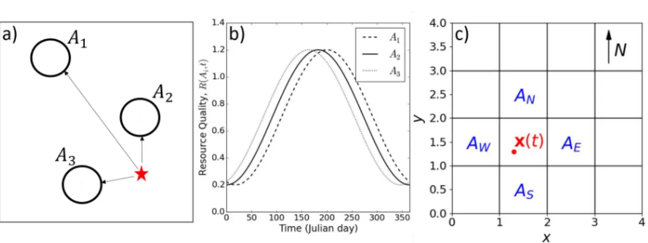
Figure 1: Panel (a) illustrates the patch selection model (Equations 1-4). Assume the

animal is at the red star. In this simplified illustration, there are just three possible

patches it can choose to move towards,

A

, A

,

and

A

(in real situations there may be

many more). The animal’s choice is determined by both the patch quality, which may

vary over time, and the distance to the patch. Panel (b) gives example curves of how

the patch quality of each patch may vary over time, each in the format of Equation (11).

Panel (c) illustrates the gradient following model (Equations 5-8). The animal is located

at position

x

(

t

) at time

t

. Patches

A

,

A

,

A

and

A

are the adjacent squares to

the patch where the animal is located.

N

,

W

,

E

,

S

stand for the north, west, east and

south respectively. When calculating the resource gradient in the nearby area of

x

(

t

), the

resource qualities in the four adjacent patches are considered, which means the animal

only assesses resource qualities in neighbouring areas to determine its moving direction.

We assume that animals move in a rasterised landscape, that is, one subdivided into a square or 173

rectangular lattice. Hereafter we will consider a square lattice for simplicity. We determine the drift 174

directionρ(t) in Equation (6) by considering the resource qualities in the four adjacent squares (North, 175

East, South, West) to the one where the animal is located. Here, the resource gradient is given as follows 176 (cf. Preisleret al.(2013)): 177 ∇w(x_{(t)) :=} w(AE)−w(AW) ∆x , w(AN)−w(AS) ∆y , (7)

where x_{(t) is the animal’s position at time t, w(AE), w(AW), w(AN), and w(AS) are the resource} 178

selection weightings (Equation 3) for the adjacent patchesAE,AW,AN andAS in the east, west, north,

179

and south respectively (Figure 1). We use ∆xto denote the distance between the centres of patchesAE

180

andAW while ∆y is the distance from the north patch to the south patch. Notice that, whilst there are

181

also diagonally adjacent squares (NW, NE, SE, SW), it is sufficient to use just four to define the resource 182

gradient, as shown in Equation (7). Then the vectorρ(t) in Equation (6) is defined as the normalised 183 vector of∇w(x_), 184 ρ(t) = ∇w( x_(t)) |∇w(x_(t))|. (8)

Note that we model our drift speed as constant (α) rather than letting it vary with the magnitude of 185

∇w(x_{). This means that the average speed of the animal across a time intervalτis kept constant, rather} 186

than being allowed to become arbitrarily large. However, the model could easily be adjusted so that 187

ρ(t) =∇w(x) if the user believes that to be more appropriate for their particular study species. 188

2.1.3

Locations between observations

In each of the above movement models, we assume that the animal can potentially make a decision 190

to reassess its movement state at any instant in continuous time. To represent this, reassessments 191

occur according to a Poisson point process with rate κ, as in Blackwell et al. (2016) (see Appendix 192

A in Supporting Information). This process means that the time intervals between reassessments are 193

exponentially distributed with parameterκ. At each reassessment time, we deterministically decide the 194

movement state, which is defined by either the attraction centreµ(t) in Equation (2) or directionρ(t) in 195

Equation (6). The movement state is decided by comparing the relative quality of resources in different 196

patches, using Equations (3-4), or calculating the resource gradient using Equation (7). 197

The fact that the choice of target location is deterministic, based on a complex evaluation of the 198

environment, contrasts with the stochastic switching of Blackwell et al. (2016), where the transition 199

rates are relatively simple functions of habitat and time. One could, in principle, extend our model so 200

that animals choose an attraction centre with a probability, based on the relative quality of each site. 201

However, this introduces extra model complexity that may not increase realism, so we have chosen to 202

model a deterministic switching process for simplicity. 203

2.2

Inference by Markov chain Monte Carlo algorithm

204

Having constructed the modelling frameworks, we use a Markov chain Monte Carlo (MCMC) algorithm, 205

based on Blackwell et al. (2016), to parameterise the models from movement data. For details of the 206

algorithm, see Appendix A in Supporting Information. 207

The MCMC algorithm comprises two main parts, one of which updates the movement trajectory by 208

simulation and the other updates parameters. To take into consideration the fact that animals can make 209

a decision to move at any time, we augment the observed data with points where the animal might have 210

changed its destination. In every iteration, we select an interval from the observed data and generate 211

a simulated path consisting of points where the switches of destinations might happen during the time 212

of the selected interval. Subsequently, we compare this simulated path with the selected interval in 213

existing trajectory by calculating the Hastings ratio, conditional on observed data points. After deciding 214

whether to accept the proposal trajectory or not, we update the parameters conditional on the accepted 215

trajectory (see Blackwellet al. (2016) for details). 216

2.3

Simulations

217

We test the MCMC algorithm on four classes of movement models. The first models migration, so 218

we assume that the animal moves in response to seasonally changing resource qualities. In the second 219

and third types of model, the resource quality depletes and renews according to the animal’s foraging 220

patterns. The last is a gradient-following model, where the animal only compares resource qualities in 221

the surrounding area to decide its direction. 222

2.3.1

Migration model

The first test of our inference method (Section 2.2) uses a very simple model of migration, whereby the 224

decision to migrate is a trade-off between the quality of a patch, which may be a destination range or 225

a stopover site, and how far it is away from the animal. Although migratory routes tend to be fixed, 226

the decision as to when to move to the next patch is not. Rather it is determined by how the quality 227

of patches over the migratory route are changing over time (e.g. due to green-up). We hypothesise that 228

movement to the next patch will occur when the animal will make sufficient foraging gains from the 229

next patch to make the movement worth while. The decision to migrate is thus caused by patch quality 230

varying over time, so we use an adjusted form of Equation (3), which includes time as a variable: 231

w(µ, t) = exp(β1R(µ, t) +β2|µ−x(t)|), (9)

wherez_{(µ, t) = (R(µ, t),|µ−}x_{(t)|) is the vector of predictor covariates withR(µ, t) the resource quality} 232

in a potential target locationµandx(t) the animal’s position at timet. We assumeβ1>0 andβ2<0,

233

representing the animal’s inclination for resources and aversion to distant places. Note that a similar 234

quality/distance trade-off for patch selection was also used by Mitchell & Powell (2004) in the slightly 235

different context of modelling home range formation. 236

In practice, since our aim is to use the patch that maximises Equation (9) as the movement centre, 237

comparing the value of Equation (9) is equivalent to comparing a constant multiple of its exponent. 238

Moreover, we can only inferβ1/β2from data instead of inferringβ1 andβ2simultaneously, because any

239

proposed values forβ1andβ2with ratio close toβ1/β2will lead to the same attraction centre. Therefore,

240

it suffices to consider a simplified version of Equation (9) as follows 241

w(µ, t) = exp(βR(µ, t)− |µ−x(t)|), (10)

whereβ =−β1/β2 is termed theresource coefficient.

242

Our model landscape consists of N non-overlapping patches, denoted by Ai, i ∈ {1,· · ·, N}. The

243

centre of patchAi is denoted byµi= (xi, yi) withy1≤y2· · · ≤yN, ordered by latitude. We assume the

244

resource quality changes periodically over the year and shifts corresponding to the latitude. The resource 245

quality R(Ai, t) in patchAi at time t (Julian day) is assumed to be a cosine function with period 365

246

days and shift controlled by (yi−y1)/(yN−y1), the relative latitude difference:

247 R(Ai, t) =acos 2π 365t− yi−y1 yN −y1 π +m, (11)

whereaand mare the amplitude and mean of resource quality andyi is they-coordinate of the centre

248

ofAi (Figure 1b).

249

We generated migration trajectories by sampling from the model described above with various values 250

of the drift coefficient,b, the diffusion coefficient,v, and the resource coefficient,βin the following ranges: 251

0.1≤b≤0.8, 2≤v≤30, and 1.5≤β ≤8.5. These are chosen to produce simulations showing migration 252

patterns on a 90×160 unit2landscape with 10 randomly generated non-overlapping food patches. These 253

implicitly include the winter and summer ranges and stopover sites between them. 254

We tested the MCMC algorithm on these simulations with resource qualities being given a priori. 255

We used a normally distributed prior for each parameter value with a mean equal to the real parameter 256

value and a standard deviation of 2. Example output is given in Figure 2a, illustrating migration from 257

the winter range in the south to the summer range in the north and back to the south over a year. We 258

used the MCMC algorithm to infer drift and diffusion coefficients (b and v respectively) from the OU 259

process in Equation (2), together with the resource coefficient, β, from the RSF in Equation (10). To 260

investigate the effectiveness of the MCMC algorithm when dealing with missing data, we carried out the 261

inference using every 5th data point, shown as red triangles in Figure 2a. We also investigated the effect 262

of finer rarification for certain simulated datasets from our study. This made very little difference to the 263

inference (details in Supplementary Appendices D-E). 264

2.3.2

Depletion-renewal models in a patchy landscape

In Section 2.3.1, we assumed that animals do not contribute in any significant way to the change of 266

resource quality (e.g. Illius et al.(2002)). In this section, we assume that the resource quality changes 267

according to the residential time of the animal in a food patch (e.g. Mitchell & Powell (2007), Van Moorter 268

et al. (2009)). As in the migration model, we describe a situation where an animal moves in pursuit 269

of quality food using the combination of the OU process and a RSF, introduced in Section 2.1.1. For 270

example, this may represent how an animal forages in its home range with complete knowledge of the 271

environment (e.g. Ford (1983)). As in Section 2.3.1, to test our inference method in a simple case, we 272

assume that the decision to move to a patch is a trade-off between the quality of a patch and the distance 273

to it and use the RSF given by Equation (10). 274

We simulate movements using Equations (2-4) in a landscape with food patchesAi,i∈ {1,· · ·, N},

275

assuming that the resources either are consumed (if the animal is present) or renewed (otherwise). 276

Specifically, if the animal is foraging in patchAi at time t, that is, x(t)∈Ai, then the resource quality

277

R(Ai, t) in patchAi decreases exponentially while those in other patches grow logistically, so that (Ford

278

(1983), Van Moorteret al.(2009)) 279 R(Aj, t+τ) =        R(Aj, t)e−djτ ifj =i, KjR(Aj, t)erjτ Kj+R(Aj, t)(erjτ−1) forj6=i, (12)

wheredj,rj andKj are the depletion rate, growth rate and carrying capacity in patchAj respectively

280

andτis a (short) time-step. For simplicity, here we assume that the growth and depletion rates and the 281

carrying capacity are the same in each patch, and thus denotedr,dandK respectively. 282

We tested the inference procedure on simulations generated with various values of the drift coefficient, 283

b, the diffusion coefficient, v, and the resource coefficient, β in the following ranges: 0.05 ≤ b ≤ 0.5, 284

1700≤v≤3500 and 0.5≤β≤5. We used a 2000×2000 unit2 landscape with 10 randomly generated 285

non-overlapping food patches. Figure 2b shows an example of simulated trajectories of movements 286

depending on resource depletion or renewal in a patchy landscape. We tested the MCMC algorithm with 287

growth (r), depletion rate (d), and carrying capacity (K) being given. We used a normally distributed 288

prior for each parameter value with a mean equal to the real parameter value and a standard deviation 289

of 2. We then inferredbandvin the OU process (Equation 2) andβin Equation (10) using the Bayesian 290

Monte Carlo algorithm. In principle, one could attempt to infer all five parameters (r, d, K, b, v) using 291

our inference procedure, but we found that it was not usually possible to obtain precise inference in 292

this case, so we would advise users to try to measurer, d,andK directly. An example of such a direct 293

method is given by Fortinet al.(2002). 294

2.3.3

Depletion-renewal models in a raster landscape

Although there are many real-life situations where resource patches are disjoint and known (e.g. Merkle 296

et al.(2014), Sawyer & Kauffman (2011)), often resources change continuously over the landscape and 297

are represented in data by a square grid (a.k.a. raster; e.g. Potts et al.(2014a)). To test whether our 298

inference procedure is effective at determining resource attraction in such situations, we model movement 299

on a square grid of resources that deplete and renew over time. In this case, the centre of each square in 300

the grid is a potential attraction centre of the OU process (Equation 2). 301

We started each simulation with homogeneous resource type in every square, which shares the same 302

carrying capacity,K, depletion and growth rates,dand r, across the land (e.g. Figure 2c). The initial 303

resource quality was equal to the carrying capacity and the resource quality in timeτfrom timetforward 304

was calculated using Equation (12) in Section 2.3.2. We tested our inference procedure on simulations 305

of the model in Equations (2-4) generated with 0.05 ≤b ≤ 0.14, 0.05 ≤v ≤0.5 and 0.2 ≤β ≤ 2 on 306

a 3×3 grid composed of unit squares. We carried out the MCMC algorithm on the assumption that 307

d, rand K are known and attempted to infer the movement coefficients b and v in the OU process in 308

Equation (2) and the resource coefficientβ in Equation (10). As for the other simulations, we used a 309

normally distributed prior for each parameter value with a mean equal to the real parameter value and 310

a standard deviation of 2. 311

2.3.4

Gradient-following models

When landscape rasters are large, it may not be computationally feasible to test every square to see if 313

it is an attractive centre. Instead, we take a different modelling approach, assuming that the animal 314

tends to move up the local resource gradient, rather than towards a prime destination. This means that 315

animals are predominantly using local perception rather than memory (cf. Bracis & Mueller (2017)). 316

Figure 2d illustrates such a trajectory in a landscape with three different resource qualities, which are 317

assumed to be static. 318

Here, the movement process is described by Equation (6) with direction corresponding to the resource 319

gradient calculated using Equations (7) and (8). We define the RSF in Equation (7) to be the resource 320

quality at a square. The parameters to be inferred areαandσfor the drift term and covariance matrix 321

in Equation (6). We tested the MCMC algorithm on simulations constructed with 0.1 ≤α, σ≤1 on a 322

10×10 grid consisting of unit squares with 3 resource qualities. As with the other simulated trajectories, 323

we used a normally distributed prior for each parameter value with a mean equal to the real parameter 324

value and a standard deviation of 2. We also compared our framework with that of Hankset al.(2015), 325

testing for both inference speed and precision by application to simulated paths (details in Supplementary 326

Appendix G). In total, for our study we analysed 45 simulated paths for the Migration model, 30 for 327

the Patch depletion/renewal model, 30 for the Raster depletion/renewal model, and 20 for the Gradient 328

following model. 329

2.4

A case study of mule deer data in the Greater Yellowstone

330

Ecosystem

331

We used GPS collar data from 28 adult (>1.5 years of age) female mule deer captured using a netgun 332

fired from a helicopter near Cody, Wyoming (USA). Collars (ATS, Iridium, Isanti, Minnesota, USA) 333

were programmed to take a fix every 2 hours, and we used data collected from March-August 2016. All 334

deer were captured following protocols consistent with the University of Wyoming standards. 335

Before employing the MCMC inference procedure introduced in Section 2.2, we identified foraging 336

patches by grouping data points where an animal stayed within a 3-km radius area for at least 3 days. 337

Subsequently, the average longitude and latitude of locations inside the patches were regarded as the 338

attraction centre (Figure 4a). For our data, these patches were quite straightforward to identify, being 339

obvious just by looking at the location data (Figure 4a; Supplementary Video SV1), and the deer have 340

high fidelity to these sites (Sawyer & Kauffman, 2011). However, this may not be true for all datasets 341

on migratory movement. For each attraction centre, we extracted the values of the normalised difference 342

vegetation index (NDVI) and instantaneous rate of green-up (IRG) for Julian days 1 to 250 from the 343

corresponding pixels in the images (Figures 4c). NDVI and IRG data were compiled from the MODIS 344

satellite based on the methods of Bischofet al.(2012) and Merkle et al.(2016). 345

Our model is based on Equation (10) for decision making and the OU process in Equation (2) for movement, and can be written out in full as follows

x_(t+τ)|x_{(t)∼M V N(µ(t) +e}−bτ_(x(t)−

µ(t)), vI(1−e−2bτ)), (13) µ(t) = argmaxi∈Ω[exp(βR(µi, t)− |µi−x(t)|)], (14)

where Ω indexes the set of attraction centres (centres of the foraging patches). We used our MCMC 346

algorithm to parameterise two different models from data. The first was the NDVI Model, whereR(µi, t)

347

is the NDVI value of patchiat timet. The second was the IRG Model, whereR(µi, t) is the IRG value

348

of patchiat timet. We used the Deviance Information Criterion (DIC) (Spiegelhalteret al.(2002)) for 349

model selection. 350

3

Results

351

3.1

Testing MCMC inference on simulations

352

3.1.1

Migration model

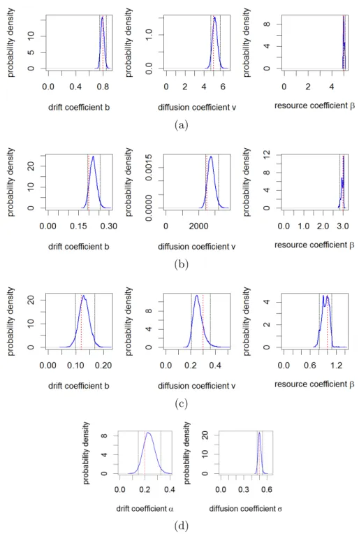
Figure 3a shows the posterior distributions derived by applying MCMC inference on the trajectory shown 354

in Figure 2a. The posterior distributions captured the real values of parameters used in simulations to 355

a good degree of accuracy with the real values lying within a 95% quantile interval of the posterior 356

distributions, indicated by black dashed lines in Figure 3a. 357

When applying the MCMC algorithm on the migration model, the sampling chains converged within 358

similar numbers of iteration in about 20 minutes (on a single thread of an i5 2.0GHz processor in a 359

Windows desktop) regardless of various values for parameters used in simulation (Figure S1 in the Sup-360

porting Information). It took longer for the chains to converge when the number of proposed switching 361

points increases (Figure S2a,b). However, the performance of estimation was not affected by the amount 362

of proposed points (Figure S2c-e). Although the value of increasing κ was insignificant here, it might 363

become important when the frequency of state switch is much higher than observation. 364

As one would expect, the chains converged faster when the initial value of the drift coefficient,b, was 365

closer to the real value, in cases when the diffusion coefficient, v, and the resource coefficient, β, were 366

fixed at real values (Figures S3a,b). However, the initial value ofv had little impact on converging time 367

(Figures S3c,d), while the chains converged faster when the initial value of β was near the real value 368

(Figures S3e,f). 369

As for accuracy, the real values ofb,vandβ were within 95% central posterior intervals of the esti-370

mated values for about 2/3, 4/5 and 1/2 simulations respectively (Figure S4, Table S1). (See Appendices 371

B, F in Supporting Information for more details.) However, where they did deviate from these intervals 372

the deviations were generally quite small (a discrepancy of less than about 25% in all cases). 373

3.1.2

Resource depletion-renewal models in a patchy landscape

The 95% central posterior interval of each posterior distribution in Figure 2b contains the real values 375

(Figure 3b), showing that our inference procedure has good accuracy in this case. 376

The algorithm was able to converge within 26,000 iterations (approximately 55 minutes) in most cases 377

(Figure S5 in the Supporting Information). It took longer for the chains to converge when the initial 378

value ofbwas far away from the real value, whereas the initial values ofv andβ had little influence on 379

the time before converging (Figure S6). Whileb andvwere captured by 95% central posterior intervals 380

for most cases, β was overestimated when the values of v or β used in simulations were higher (Figure 381

S7, Table S1) (See Appendix C in Supporting Information for more details.) 382

3.1.3

Resource depletion-renewal models in a raster landscape

For the case shown in Figure 2c, the posterior distributions captured parameters successfully, as shown 384

in Figure 3c, despite that it is not straightforward to identify the attraction centres simply by eyeballing 385

the trajectory. 386

In general, the convergence time of the algorithm was independent of the values of coefficients used 387

in simulations (Figures S8 in the Supporting Information). However, starting the algorithm with initial 388

values closer to real values usually led to faster convergence, as one would expect (Figure S9). 389

The performance of the MCMC algorithm using every 5th data point was similar to that using 390

every 3rd point, but the discrepancy between sample means ofβ and real values was lower when more 391

observations were considered (Figures S10,11,12). (See Appendix D in Supporting Information for more 392

details.) 393

3.1.4

Gradient-following models

In the case shown in Figure 2d, the posterior distributions successfully captured the real values within 395

95% central posterior intervals. 396

The value of the drift speed, α, used to generate a simulated trajectory had no obvious impact on 397

the time when MCMC chains converged (Figure S13a in the Supporting information). On the other 398

hand, the chains tended to converge quicker when largerσwas used in simulation (Figure S13b). There 399

was no clear relationship between the convergence time and initial values for the MCMC algorithm when 400

inferring parameters from the simulation in Figure 2d (Figure S14). Initial values near real values did 401

not guarantee faster convergence. On the contrary, the algorithm converged after fewer iterations when 402

the initial values of αwere more than 10 times larger than the real value (Figure S14b). This might 403

result from the slower convergence of the sampling chain ofσ, which dominated the overall converging 404

time, and fluctuations in the chains caused by the augmentation of data points. In general, the accuracy 405

of estimatingσimproved significantly when more data points were used in the inference procedure, while 406

the accuracy of estimatingαwas less affected by the density of data (Figures S15,16). (See Appendix 407

E in Supporting Information for more details.) Our comparison with the method of Hankset al.(2015) 408

reveals that our method shows that our method is more precise (e.g. the posterior standard deviation of 409

αwas more than an order of magnitude smaller than the equivalent measure from the model of Hanks 410

et al.(2015)) on data simulated from our model. 411

3.2

Applying MCMC inference on the mule deer data

412

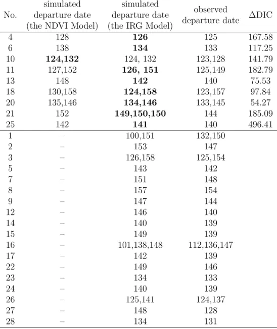
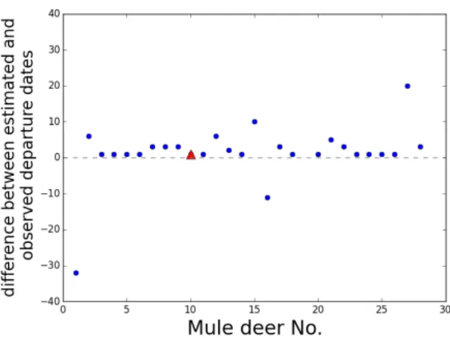
When fitting the IRG Model to the deer data, the MCMC algorithm converged for 27 of the 28 individuals, 413

whereas the NDVI Model only converged for 9. This gives some preliminary indication that the NDVI 414

model is not a good model for these data. In the 9 cases where both the NDVI and IRG Models led to 415

convergent MCMC results (e.g. No. 4, Table 1), the DIC was used to determine the better model. This 416

reveals that the NDVI Model is a better fit for one of the deer (No. 10) and the IRG Model for the other 417

eight (Table 1), confirming our preliminary indications. For those cases where MCMC chains converged, 418

we used the posterior mean of β of the best fit model to calculate the simulated departure dates of 419

migration, shown together with the real departure dates in Table 1. The estimated departure dates were 420

defined to be the dates when a switch of movement centre had occurred according to the RSF. The 421

observed departure dates were the dates when locations occurring outside a patch and towards another 422

patch were first observed. The agreement was generally good, suggesting that, when a model can be 423

fitted to the data, the timing of migration can be explained by a simple trade-off between relative NDVI 424

or IRG values and the distance between successive patches, but usually IRG is a better measurement to 425

use (Figure 5). 426

However, for one individual (No. 21, Table 1), the inference procedure estimated that the individual 427

left a patch, and was attracted to it again for a very short time soon after migrating. This is probably 428

not a behavioural feature, though, since it was not observed in the data. Rather, this is likely to be a 429

quirk resulting from small up-and-down fluctuation in the IRG around the time of migration. 430

Figure 4a gives an example migratory path of an individual, which can be compared with the 431

simulated path from the best-fit model (Figure 4b). Supplementary Video SV1 shows an animation of 432

both these paths superimposed (red dots are the observed locations and blue are simulated). In the 433

best-fit model, the attraction centre changed fromµ1 toµ2on the 126th day of the year (Table 1). This

434

is very close to the actual date of departure from winter range observed from data and is marked by an 435

arrow in Figure 4c. Finally, the posterior distributions for this example are given in Figure 4d, where 436

we observe a significant difference between the posterior mean and zero for each parameter (p <10−5

). 437

4

Discussion

438

We have constructed models of resource selection in continuous time, based on a switching random walk 439

process, and parameterised using a Bayesian Monte Carlo algorithm. We have demonstrated that our 440

method can be applied in a wide range of scenarios, including both movements driven by the evaluation 441

of resources at the landscape scale, and those that simply follow local resource gradients. In broad terms, 442

our model animals first (a) assess location and quality of different resources (either proximately or across 443

the whole landscape), to decide the general direction of movement, then (b) move according to a process 444

that incorporates not only the resource-based decision, but also some stochasticity to account for any 445

unknown factors governing movement. Such stochastic continuous-time models allow us to make use 446

of well-developed, flexible inference procedures (Blackwellet al. (2016)). When applying our inference 447

No.

simulated

departure date

(the NDVI Model)

simulated

departure date

(the IRG Model)

observed

departure date

∆DIC

4

128

126

125

167.58

6

138

134

133

117.25

10

124,132

124, 132

123,128

141.79

11

127,152

126, 151

125,149

182.79

13

148

142

140

75.53

18

130,158

124,158

123,157

97.84

20

135,146

134,146

133,145

54.27

21

152

149,150,150

144

185.09

25

142

141

140

496.41

1

–

100,151

132,150

2

–

153

147

3

–

126,158

125,154

5

–

143

142

7

–

151

148

8

–

157

154

9

–

147

144

12

–

146

140

14

–

140

139

15

–

149

139

16

–

101,138,148

112,136,147

17

–

142

139

22

–

149

146

23

–

134

133

24

–

140

139

26

–

125,141

124,137

27

–

148

128

28

–

134

131

Table 1: The comparison of models for the mule deer data. For cases where the switch of

movement centre occurred on two days, the numbers for the Julian dates are separated

with a comma. Figures in bold indicate the model with smaller DIC value on that

individual.

algorithm to simulated data, where all the parameter values governing the movement are known, we 448

were able to estimate the input parameters, including those governing the trade-off between maximising 449

resource intake and minimising travel costs, with good accuracy. As such, our method can reliably 450

capture important aspects of the processes underlying movement decisions. 451

Our framework can be viewed as generalising ideas from several previous studies. The study of 452

Hankset al.(2015) developed a gradient following algorithm that allows for behavioural switches between 453

observed locations. This is similar to our gradient-following model, yet relies upon discretising the path 454

into presence or absence on pixels of a square lattice, whereas ours considers the full, continuous path. A 455

comparison of our method with that of Hankset al.(2015) on a path simulated from our model revealed 456

that in this case our method is more precise. However, this is not surprising, as we would expect a better 457

fit from a model that accurately mimics the true movement process. Employing the model in Hankset al. 458

(2015), Brennanet al.(2018) attempted better understanding of habitat preferences by considering the 459

impact of corridor choice on speed during migration, while we focus on the movement direction decided 460

by identifying the destination. Breedet al. (2017) gives a model of patch-to-patch movement, based on 461

a switching OU process, but where only the decision toleavea patch depends on environmental features. 462

Ours generalises this by modelling patch-to-patch movements as dependent on the source patch, the 463

target patch, and the distance between them. 464

In this study, we have examined gradient-following and patch selection models separately. In prin-465

ciple, it would be possible to combine these. One would begin by writing down a stochastic differential 466

equation that combines the processes in Equations (1) and (5) then derive from these the distribution of 467

movement across a short time-interval (similar to Equations 2 and 6). This distribution can then be fed 468

into the inference algorithm described in Section 2.2. Of course, such a model would be more complex 469

than those described here, so would likely require more running time and a good dataset to achieve 470

accurate inference. 471

We have focused on a few simple situations where the main factor in movement decisions is resource 472

quality. However, being based on a resource selection function (RSF), our framework has potential 473

to incorporate as wide a variety of movement covariates as in traditional resource- or step-selection 474

analysis. For example, topography (Potts et al. (2014c)), interactions between animals (Vanak et al. 475

(2013)), memory effects (Merkle et al. (2017)), barriers and corridors (Panzacchi et al. (2016)) have 476

all been incorporated into step-selection analysis and so could, in principle, be incorporated into our 477

modelling framework. 478

Classical step selection analysis tends to examine resource selection from one measured location to 479

the next (Thurfjell et al. (2014)). However, it has occasionally been used to measure patch-to-patch 480

movements (e.g. Merkleet al. (2014)) and this is similar in flavour to our patch-based models. On the 481

other hand, our raster-based models are more appropriate for studies where distinct patches are less 482

clear. In this case, it is often far less clear what spatio-temporal scales are being used by the animal 483

to make selection decisions. However, to use step selection analysis, one is forced either to make an 484

a priori choice of scale or perform a complicated model selection procedure (Bastille-Rousseau et al. 485

(2018)). Our approach has the advantage that the spatio-temporal scale of decision-making emerges 486

from the interface between the landscape and the movement processes, and is not tied to the frequency 487

of the location data. In addition, the flexibility of the switching random walk framework means that 488

our models have potential to include variation in behavioural modes in different parts of space (Harris & 489

Blackwell (2013)) or in different states such as encamped and exploratory states (Moraleset al.(2004)). 490

Indeed, the switching OU framework used here has recently been used to model state-switching 491

correlated random walks (Michelot & Blackwell (2019)). This makes use of the same code base as the 492

code used for inference here, so is ready to be combined with our models. Furthermore, although we 493

have developed our techniques for use with single animal tracks, there is ongoing work to incorporate 494

collective movement and animal interactions into the switching OU framework (Niuet al.(2016)), which 495

could be important for the study of mule deer (Sawyer et al., 2006). Therefore we intend for future 496

studies to factor group movement into continuous-time resource selection. 497

To demonstrate how our techniques can be applied to real data, we assessed the underlying mecha-498

nisms behind migration in mule deer. Our results support two hypotheses related to migration. First is 499

the Forage Maturation Hypothesis, which posits that as plants grow herbivores face a trade-off between 500

forage quality and quantity and therefore will select forage patches at intermediate stages of growth 501

(Fryxell (1991), Hebblewhiteet al.(2008)). Second is the Green Wave Hypothesis (Drentet al.(1978)), 502

which is the spatial manifestation of the Forage Maturation Hypothesis (Merkle et al. (2016)). The 503

Green Wave Hypothesis posits that animals migrate to acquire high-quality foods that are propagated 504

as resource waves in space and time. For migratory herbivores, resource waves often correspond to the 505

onset of spring along the migration route (Aikenset al.(2017)). The Green Wave Hypothesis has been 506

tested in a variety of species of both birds and mammals (van Wijket al. (2012), K¨olzschet al.(2015), 507

Merkleet al.(2016)). 508

We used a model where the animal trades-off the relative quality of resources at source and target 509

locations with the effort of moving from one to the other (using distance between patches as a proxy for 510

effort). We used two proxies for resource quality of a patch: NDVI and IRG. The former represents an 511

index of green forage biomass, and the latter represents an index of intermediate forage biomass (Bischof 512

et al.(2012)). Similar to the findings of Aikenset al.(2017) and Merkle et al.(2016) for mule deer, our 513

results suggest that the movements of most individual mule deer could be explained by IRG. The use 514

of growthrate(IRG), rather thanabsolutequality of biomass (NDVI) suggests that movement is caused 515

predominantly by theprocessof change, i.e. green-up. This is consistent with the idea of ‘surfing a green 516

wave’: tracking the places at which rate of change is greatest. Note that for one individual, however, 517

the model using NDVI did fit better (No. 10, Table 1). Nonetheless, the resulting best-fit models 518

tend to anticipate the migratory times well (Table 1, Figure 5), and simulated paths are qualitatively 519

similar to the real paths (Supplementary Video SV1). Therefore our method has potential to test various 520

hypotheses explaining migratory movement, and resource-driven movement in general. 521

In conclusion, we have developed a flexible framework for continuous-time inference of resource 522

selection decisions in moving animals. The switching random-walk model, combined with Bayesian 523

Monte Carlo inference, generalises several previous methods, and has potential to be extended to a wide 524

range of scenarios. Whilst the inference speed is sufficient for paths of several hundred data-points, it 525

may prove too slow with modern-era tracks that can contain millions (Hays et al.(2016)). Therefore a 526

significant future challenge would be to develop either methods for speeding-up inference significantly 527

(K´alm´an filters may be an appropriate technique here: e.g. Fleming et al. (2017)), or rarefying high-528

resolution data to extract key locations in the path that represent animal decisions (Pottset al.(2018)). 529

Indeed, the key limiting factor for speed is the number of MCMC samples required for convergence. 530

Better data, sampled at behaviourally-meaningful locations, may have a clearer signal thus requiring 531

less time for the MCMC procedure to converge, even if the datasets might be larger. In summary, 532

our framework represents an important methodological step in understanding resource-use decisions by 533

moving animals. 534

Acknowledgements

535

This work is supported in part by a scholarship provided by Ministry of Education of Taiwan (YW). 536

We thank Mu Niu and Th´eo Michelot for contributions to the code that we adapted in building our 537

inference procedure. Collection of the mule deer data was supported by the Wyoming Game and Fish 538

Department, the Nature Conservancy of Wyoming, and the Knobloch Family Foundation. We thank two 539

anonymous reviewers, an associate editor and the senior editor, Bob O’Hara, for comments that have 540

helped improve the manuscript. 541

Author Contributions

542

JRP, PGB conceived and designed the research; YW performed the research; JAM provided data; PGB 543

provided code for inference; YW, JRP led the writing of the manuscript. All authors contributed critically 544

to the drafts and gave final approval for publication. 545

Data Accessibility

546

Data used in this manuscript are archived on Data Dryad atdoi:10.5061/dryad.f9p3dq4. 547

References

548

1. 549

Aikens, E.O., Kauffman, M.J., Merkle, J.A., Dwinnell, S.P., Fralick, G.L. & Monteith, K.L. (2017). 550

The greenscape shapes surfing of resource waves in a large migratory herbivore. Ecol. Lett., 20, 551

741–750. 552

2. 553

Avgar, T., Lele, S.R., Keim, J.L. & Boyce, M.S. (2017). Relative Selection Strength: Quantifying 554

effect size in habitat- and step-selection inference. Ecol Evol, 7, 5322–5330. 555

3. 556

Avgar, T., Potts, J.R., Lewis, M.A. & Boyce, M.S. (2016). Integrated step selection analysis: bridging 557

the gap between resource selection and animal movement. Methods Ecol Evol, 7, 619–630. 558

4. 559

Bastille-Rousseau, G., Murray, D.L., Schaefer, J.A., Lewis, M.A., Mahoney, S.P. & Potts, J.R. (2018). 560

Spatial scales of habitat selection decisions: implications for telemetry-based movement modelling. 561

Ecography, 41, 437–443. 562

5. 563

Bastille-Rousseau, G., Potts, J.R., Schaefer, J.A., Lewis, M.A., Ellington, E., Rayl, N., Mahoney, 564

S. & Murray, D.L. (2015). Unveiling trade-offs in resource selection of migratory caribou using a 565

mechanistic movement model of availability. Ecography, 38, 1049–1059. 566

6. 567

Bischof, R., Loe, L.E., Meisingset, E.L., Zimmermann, B., Van Moorter, B. & Mysterud, A. (2012). 568

A migratory northern ungulate in the pursuit of spring: jumping or surfing the green wave? Am. 569

Nat., 180, 407–424. 570

7. 571

Blackwell, P.G. (1997). Random diffusion models for animal movement. Ecol Modell, 100, 87–102. 572

8. 573

Blackwell, P.G. (2003). Bayesian inference for Markov processes with diffusion and discrete compo-574

nents. Biometrika, 90, 613–627. 575

9. 576

Blackwell, P.G., Niu, M., Lambert, M.S. & LaPoint, S.D. (2016). Exact Bayesian inference for animal 577

movement in continuous time. Methods Ecol Evol, 7, 184–195. 578

10. 579

Boyce, M.S. (2006). Scale for resource selection functions. Diversity Distrib., 12, 269–276. 580

11. 581

Boyce, M.S., Vernier, P.R., Nielsen, S.E. & Schmiegelow, F.K. (2002). Evaluating resource selection 582

functions. Ecol Modell, 157, 281–300. 583

12. 584

Bracis, C. & Mueller, T. (2017). Memory, not just perception, plays an importnat role in terrestrial 585

mammalian migration. Proc. R. Soc. B, 284, 20170449. 586

13. 587

Breed, G.A., Golson, E.A. & Tinker, M.T. (2017). Predicting animal home-range structure and 588

transitions using a multistate Ornstein-Uhlenbeck biased random walk. Ecology, 98, 32–47. 589

14. 590

Brennan, A., Hanks, E.M., Merkle, J.A., Cole, E.K., Dewey, S.R., Courtemanch, A.B. & Cross, P.C. 591

(2018). Examining speed versus selection in connectivity models using elk migration as an example. 592

Landscape Ecol, 33, 955–968. 593

15. 594

Cagnacci, F., Boitani, L., Powell, R.A. & Boyce, M.S. (2010). Animal ecology meets GPS-based 595

radiotelemetry: a perfect storm of opportunities and challenges. Phil. Tran. R. Soc. B, 365, 2157– 596

2162. 597

16. 598

Chetkiewicz, C.L.B. & Boyce, M.S. (2009). Use of resource selection functions to identify conservation 599

corridors. J. Appl. Ecol., 46, 1036–1047. 600

17. 601

Drent, R., Ebbinge, B. & Weijand, B. (1978). Balancing the energy budgets of arctic-breeding geese 602

throughout the annual cycle: a progress report. Verh. Ornithol. Ges. Bayern., 23, 239–264. 603

18. 604

Fleming, C.H., Sheldon, D., Gurarie, E., Fagan, W.F., LaPoint, S. & Calabrese, J.M. (2017). K´alm´an 605

filters for continuous-time movement models. Ecol. Inform., 40, 8–21. 606

19. 607

Ford, R.G. (1983). Home range in a patchy environment: optimal foraging predictions.Integr. Comp. 608

Biol., 23, 315–326. 609

20. 610

Forester, J., Im, H. & Rathouz, P. (2009). Accounting for animal movement in estimation of resource 611

selection functions: sampling and data analysis. Ecology, 90, 3554–3565. 612

21. 613

Fortin, D., Beyer, H., Boyce, M.S., Smith, D., Duchesne, T. & Mao, J.S. (2005). Wolves influence elk 614

movements: behavior shapes a trophic cascade in Yellowstone National Park.Ecology, 86, 1320–1330. 615

22. 616

Fortin, D., Fryxell, J.M. & Pilote, R. (2002). The temporal scale of foraging decisions in bison.Ecology, 617

83, 970–982. 618

23. 619

Fryxell, J.M. (1991). Forage quality and aggregation by large herbivores. Am. Nat., 138, 478–498. 620

24. 621

Hanks, E.M., Hooten, M.B. & Alldredge, M.W. (2015). Continuous-time discrete-space models for 622

animal movement. Ann. Appl. Stat., 9, 145–165. 623

25. 624

Hanks, E.M., Hooten, M.B., Johnson, D.S. & Sterling, J.T. (2011). Velocity-based movement modeling 625

for individual and population level inference. PLOS ONE, 6, e22795. 626

26. 627

Harris, K.J. & Blackwell, P.G. (2013). Flexible continuous-time modelling for heterogeneous animal 628

movement. Ecol Modell, 255, 29–37. 629

27. 630

Hays, G., Ferreira, L., Sequeira, A., Meekan, M., Duarte, C., Bailey, H., Bailleul, F., Bowen, W., 631

Caley, M. & Costa, D. (2016). Key questions in marine megafauna movement ecology. Trends Ecol. 632

Evol., 31, 463–475. 633

28. 634

Hebblewhite, M., Merrill, E. & McDermid, G. (2008). A multi-scale test of the forage maturation 635

hypothesis in a partially migratory ungulate population. Ecol. Monogr., 78, 141–166. 636

29. 637

Hooten, M.B., Johnson, D.S., Hanks, E.M. & Lowry, J.H. (2010). Agent-based inference for animal 638

movement and selection. J Agric Biol Environ Stat, 15, 523–538. 639

30. 640

Illius, A.W., Duncan, P., Richard, C. & Mesochina, P. (2002). Mechanisms of functional response and 641

resource exploitation in browsing roe deer. J. Anim. Ecol., 71, 723–734. 642

31. 643

Johnson, D.S., Thomas, D.L., Ver Hoef, J.M. & Christ, A. (2008). A general framework for the 644

analysis of animal resource selection from telemtry data. Biometrics, 64, 968–976. 645

32. 646

K¨olzsch, A., Bauer, S., Boer, R., Griffin, L., Cabot, D., Exo, K.M., van der Jeugd, H.P. & Nolet, 647

B.A. (2015). Forecasting spring from afar? Timing of migration and predictability of phenology along 648

different migration routes of an avian herbivore. J. Anim. Ecol., 84, 272–283. 649

33. 650

Lendrum, P.E., Anderson Jr., C.R., Long, R.A., Kie, J.G. & Bowyer, R.T. (2012). Habitat selection 651

by mule deer during migration: effects of landscape structure and natural-gas development.Ecosphere, 652

3, 82. 653

34. 654

Manly, B., McDonald, L., Thomas, D., McDonald, T. & Erickson, W. (2002). Resource selection by 655

animals: statistical analysis and design for field studies. 2nd edn. Springer Netherlands. 656

35. 657

McClintock, B.T., Johnson, D.S., Hooten, M.B., Ver Hoef, J.M. & Morales, J.M. (2014). When to be 658

discrete: the importance of time formulation in understanding animal movement. Movement Ecol, 2. 659

36. 660

McLoughlin, P.D., Morris, D.W., Fortin, D., Vander Wal, E. & Contasti, A.L. (2010). Considering 661

ecological dynamics in resource selection functions. J. Anim. Ecol., 79, 4–12. 662

37. 663

Merkle, J.A., Cross, P., Scurlock, B.M., Cole, E., Courtemanch, A., Dewey, S. & Kauffman, M.J. 664

(2018). Linking spring phenology with mechanistic models of host movement to predict disease trans-665

mission risk. J. Appl. Ecol., 55, 810–819. 666

38. 667

Merkle, J.A., Fortin, D. & Morales, J.M. (2014). A memory-based foraging tactic reveals an adaptive 668

mechanism for restricted space use. Ecol Lett, 17, 924–931. 669

39. 670

Merkle, J.A., Monteith, K.L., Aikens, E.O., Hayes, M.M., Hersey, K.R., Middleton, A.D., Oates, B.A., 671

Sawyer, H., Scurlock, B.M. & Kauffman, M.J. (2016). Large herbivores surf waves of green-up during 672

spring. Proc. R. Soc. B, 283, 20160456. 673

40. 674

Merkle, J.A., Potts, J.R. & Fortin, D. (2017). Energy benefits and emergent space use patterns of an 675

empirically parameterized model of memory-based patch selection. Oikos, 126. 676

41. 677

Michelot, T. & Blackwell, P.G. (2019). State-switching continuous-time correlated random walks. 678

Methods in Ecology and Evolution. 679

42. 680

Michelot, T., Blackwell, P.G. & Matthiopoulos, J. (2018). Linking resource selection and step selection 681

models for habitat preferences in animals. Ecology. Accepted Author Manuscript. 682

43. 683

Mitchell, M.S. & Powell, R.A. (2004). A mechanistic home range model for optimal use of spatially 684

distributed resources. Ecol. Modell., 177, 209–232. 685

44. 686

Mitchell, M.S. & Powell, R.A. (2007). Optimal use of resources structures home ranges and spatial 687

distribution of black bears. Anim. Behav., 74, 219–230. 688

45. 689

Moorcroft, P. & Barnett, A. (2008). Mechanistic home range models and resource selection analysis: 690

a reconciliation and unification. Ecology, 89, 1112–1119. 691

46. 692

Morales, J.M., Haydon, D.T., Frair, J., Holsinger, K.E. & Fryxell, J.M. (2004). Extracting more out 693

of relocation data: building movement models as mixtures of random walks. Ecology, 85, 2436–2445. 694

47. 695

Niu, M., Blackwell, P.G. & Skarin, A. (2016). Modeling interdependent animal movement in continuous 696

time. Biometrics, 72, 315–324. 697