Digital Object Identifier (DOI) 10.1007/s00220-009-0754-z
Mathematical
Physics
On the Mean-Field Limit of Bosons
with Coulomb Two-Body Interaction
Jürg Fröhlich, Antti Knowles, Simon Schwarz
Institute of Theoretical Physics, ETH Hönggerberg, CH-8093 Zürich, Switzerland. E-mail: juerg@itp.phys.ethz.ch; aknowles@itp.phys.ethz.ch; sschwarz@itp.phys.ethz.ch Received: 28 May 2008 / Accepted: 2 December 2008
Published online: 28 February 2009 – © Springer-Verlag 2009
Abstract: In the mean-field limit the dynamics of a quantum Bose gas is described by a Hartree equation. We present a simple method for proving the convergence of the microscopic quantum dynamics to the Hartree dynamics when the number of particles becomes large and the strength of the two-body potential tends to 0 like the inverse of the particle number. Our method is applicable for a class of singular interaction potentials including the Coulomb potential. We prove and state our main result for the Heisenberg-picture dynamics of “observables”, thus avoiding the use of coherent states. Our formu-lation shows that the mean-field limit is a “semi-classical” limit.
1. Introduction
Whenever many particles interact by means of weak two-body potentials, one expects that the potential felt by any one particle is given by an average potential generated by the particle density. In this mean-field regime, one hopes to find that the emerging dynamics is simpler and less encumbered by tedious microscopic information than the original N -body dynamics.
The mathematical study of such problems has quite a long history. In the context of classical mechanics, where the mean-field limit is described by the Vlasov equation, the problem was successfully studied by Braun and Hepp [3], as well as Neunzert [16]. The mean-field limit of quantum Bose gases was first addressed in the seminal paper [10] of Hepp. We refer to [6] for a short discussion of some subsequent results. The case with a Coulomb interaction potential was treated by Erd˝os and Yau in [6]. Recently, Rodnianski and Schlein [21] have derived explicit estimates for the rate of convergence to the mean-field limit, using the methods of [10and9]. A sharper bound on the rate of convergence in the case of a sufficiently regular interaction potential was derived by Schlein and Erd˝os [22], by using a new method inspired by Lieb-Robinson inequalities. In [7,15], the mean-field limit (N → ∞) and the classical limit were studied simultaneously. A conceptually quite novel approach to studying mean-field limits was introduced in [8].
In that paper, the time evolution of quantum and corresponding “classical” observables is studied in the Heisenberg picture, and it is shown that “time evolution commutes with quantisation” up to terms that tend to 0 in the mean-field (“classical”) limit, which is a
Egorov-type result.
In this paper we present a new, simpler way of handling singular interaction poten-tials. It yields a Egorov-type formulation of convergence to the mean-field limit, thus obviating the need to consider particular (traditionally coherent) states as initial con-ditions. Another, technical, advantage of our method is that it requires no regularity (traditionally H1- or H2-regularity) when applied to coherent states.
Such kinds of results were first obtained by Egorov [5] for the semi-classical limit of a quantum system. Roughly, the statement is that time-evolution commutes with quanti-sation in the semi-classical limit. We sketch this in a simple example: Let us start with a classical Hamiltonian system of a finite number f of degrees of freedom. The classical algebra of observablesAis given by (some subalgebra of) the Abelian algebra of smooth functions on the phase space :=R2 f. Let H ∈ Abe a Hamilton function. Together with the symplectic structure on, H generates a symplectic flowφt on. Now we define a quantisation map(·):A→A, whereAis some subalgebra ofB(L2(Rf)). For concreteness, let(·)be Weyl quantisation with deformation parameter. This implies that
A,B =
i{A,B}+ O(
2),
for→0. The quantised Hamilton function defines a 1-parameter group of automor-phisms onAthrough
A → eitH/A e−itH/, A∈A.
A Egorov-type semi-classical result states that, for all A∈Aand t ∈R,
(A◦φt)
= eitH/Ae−itH/
+ R(t),
whereR(t) →0 as→0.
This approach identifies the semi-classical limit as the converse of quantisation. In a similar fashion, we identify the mean-field limit as the converse of “second quantisa-tion”. In this case the deformation parameter is not, but N−1, a parameter proportional to the coupling constant. We consider the mean-field dynamics (given by the Hartree equation in the case of bosons), and view it as the Hamiltonian dynamics of a classical Hamiltonian system. We show that its quantisation describes N -body quantum mechan-ics, and that the “semi-classical” limit corresponding to N−1→0 takes us back to the Hartree dynamics.
We sketch the key ideas behind our strategy.
(1) Use the Schwinger-Dyson expansion to construct the Heisenberg-picture dynamics of p-particle operators
eit HNA
N(a(p))e−it HN
(in the notation of Sect.3).
(2) Use Kato smoothing plus combinatorial estimates (counting of graphs) to prove convergence of the Schwinger-Dyson expansion on N -particle Hilbert space, uni-formly in N and for small|t|. Diagrams containing l loops yield a contribution of
(3) Use Kato smoothing plus combinatorial estimates to prove convergence of the iterative solution of the Hartree equation, for small|t|.
(4) Show that the Wick quantisation of the series in (3) is equal to the series of tree diagrams in (2).
(5) Extend (2) and (3) to arbitrary times by using unitarity and conservation laws. This paper is organised as follows. In Sect.2we show that the classical Newtonian mechanics of point particles is the second quantisation of Vlasov theory, the latter being the mean-field (or “classical”) limit of the former. The bulk of the paper is devoted to a rigorous analysis of the mean-field limit of Bose gases. In Sect.3we recall some impor-tant concepts of quantum many-body theory and introduce a general formalism which is convenient when dealing with quantum gases. Section4contains an implementation of Step (1) above. The convergence of the Schwinger-Dyson series for bounded inter-action potentials is briefly discussed in Sect.5. Section6implements Step (2) above. Steps (3), (4) and (5) are implemented in Sect.7. Finally, Sect.8extends our results to more general interaction potentials as well as nonvanishing external potentials.
2. Mean-Field Limit in Classical Mechanics
In this section we consider the example of classical Newtonian mechanics to illustrate how the atomistic constitution of matter arises by quantisation of a continuum theory. The aim of this section is to give a brief and nonrigorous overview of some ideas that we shall develop in the context of quantum Bose gases, in full detail, in the following sections.
A classical gas is described as a continuous medium whose state is given by a non-negative mass density dµ(x, v) = M f(x, v)dx dv on the “one-particle” phase space R3×R3. Here M is the mass of one “mole” of gas;µ(A)is the mass of gas in the
phase space volume A⊂R3×R3. Letdx dv f(x, v)=ν <∞denote the number of “moles” of the gas, so that the total mass of the gas isµ(R3×R3)=νM. An example
of an equation of motion for f(x, v)is the Vlasov equation
∂tft(x, v) = −(v· ∇xft) (x, v)+
1
m (∇Veff[ft] · ∇vft) (x, v), (2.1)
where m is a constant with the dimension of a mass, t denotes time, and
Veff[f](x) = V(x)+
dy W(x−y)
dv f(y, v).
Here V is the potential of external forces acting on the gas and W is a (two-body) potential describing self-interactions of the gas.
The Vlasov equation arises as the mean-field limit of a classical Hamiltonian sys-tem of n point particles of mass m, with trajectories(xi(t))ni=1, moving in an external potential V and interacting through two-body forces with potential N−1W(xi −xj).
Here N is the inverse coupling constant. We interpret N as “Avogadro’s number”, i.e. as the number of particles per “mole” of gas. Thus, M =m N and n=νN . More precisely,
it is well-known (see [3,16]) that, under some technical assumptions on V and W ,
ft(x, v) = w*-lim n→∞ ν n n i=1 δ(x−xi(t)) δ(v− ˙xi(t)) (2.2)
exists for all times t and is the (unique) solution of (2.1), provided that this holds at time t =0. Here, ft is viewed as an element of the dual space of continuous bounded
functions.
Note that n and N are, a priori, unrelated objects. While n is the number of particles in the classical Hamiltonian system, N−1 is by definition the coupling constant. The mean-field limit is the limit n→ ∞while keeping n∝ N ; the proportionality constant
isν.
It is of interest to note that the Vlasov dynamics (2.1) may be interpreted as a Hamiltonian dynamics on an infinite-dimensional affine phase space Vlasov. To see
this, we write
f(x, v) = ¯α(x, v)α(x, v),
whereα(¯ x, v), α(x, v)are complex coordinates onVlasov. For our purposes it is enough
to say thatVlasovis some dense subspace of L2(R6)(typically a weighted Sobolev space
of index 1). OnVlasovwe define a symplectic form through
ω = i
dx dvdα(¯ x, v)∧dα(x, v).
This yields a Poisson bracket which reads
α(x, v), α(y, w)=α(¯ x, v),α(¯ y, w) = 0,
α(x, v),α(¯ y, w)=iδ(x−y)δ(v−w). (2.3)
A Hamilton function H is defined onVlasovthrough H(α):=i dx dvα(¯ x, v) −v· ∇x+ 1 m∇V(x)· ∇v α(x, v) + i m dx dvα(¯ x, v) dy dw∇W(x−y)|α(y, w)|2 · ∇vα(x, v).(2.4) Note that H is invariant under gauge transformationsα→e−iθα,α¯ →eiθα¯, which by Noether’s theorem implies that|α|2dx dv= f dx dvis conserved.
Let us abbreviate K := −∇V/m and F := −∇W/m. After a short calculation using
(2.3) we find that the Hamiltonian equation of motionα˙t(x, v) = {H, αt(x, v)}reads
˙ αt(x, v)=(−v· ∇x−K(x)· ∇v) αt(x, v)− dy dw F(x−y)|αt(y, w)|2· ∇vαt(x, v) + dy dw F(x−y)α¯t(y, w)αt(x, v)· ∇wαt(y, w). (2.5)
Also,α¯tsatisfies the complex conjugate equation. Therefore,
d dt|αt(x, v)| 2=(−v· ∇ x−K(x)· ∇v)|αt(x, v)|2 − dy dw F(x−y)|αt(y, w)|2· ∇v|αt(x, v)|2 +|αt(x, v)|2 dy dwF(x−y) ·α¯t(y, w)∇wαt(y, w)+αt(y, w)∇wα¯t(y, w) . (2.6)
We assume that
|α(x, v)| = o(|(x, v)|−1), (x, v)→ ∞. (2.7)
We shall shortly see that this property is preserved under time-evolution. By integra-tion by parts, we see that the second line of (2.6) vanishes, and we recover the Vlasov equation of motion (2.1) for f = |α|2.
We comment briefly on the existence and uniqueness of solutions to the Hamiltonian equation of motion (2.5). Following Braun and Hepp [3], we assume that K and F are bounded and continuously differentiable with bounded derivatives. We use polar coordinates
α = βeiϕ,
whereϕ∈Randβ ≥0. Then the Hamiltonian equation of motion (2.5) reads ˙ βt(x, v)=(−v· ∇x−K(x)· ∇v) βt(x, v) − dy dwF(x−y) βt2(y, w)· ∇vβt(x, v), (2.8a) ˙ ϕt(x, v)=(−v· ∇x−K(x)· ∇v) ϕt(x, v)− dy dwF(x−y) βt2(y, w)· ∇vϕt(x, v) + dy dw F(x−y) βt2(y, w)· ∇wϕt(y, w). (2.8b)
We consider two cases.
(i) ϕ = 0. In this caseα = β and the equations of motion (2.8) are equivalent to the Vlasov equation for f = β2. The results of [3,16] then yield a global well-posedness result.
(ii) ϕ =0. The equation of motion (2.8a) is independent ofϕ. Case (i) implies that it has a unique global solution. In order to solve the linear equation (2.8b), we apply a contraction mapping argument. Consider the space X := {ϕ∈C(R6) : ∇ϕ ∈ L∞(R6)}. Using Sobolev inequalities one finds that X , equipped with the norm
ϕX := |ϕ(0)|+∇ϕ∞, is a Banach space. We rewrite (2.8b) as an integral
equation, and using standard methods show that, for small times, it has a unique solution. Using conservation ofdx dv βt2we iterate this procedure to find a global solution. We omit further details.
Note that, as shown in [3], the solutionβt can be written using a flow φt on the
one-particle phase space:βt(x, v) =β0(φ−t(x, v)). The flowφt(x, v) =(x(t), v(t))
satisfies ˙ x(t)=v(t), ˙ v(t)=K(x(t))+ dy dw βt2(y, w)F(x(t)−y).
Using conservation ofdx dv βt2we find that there is a constant C such that|φ−t(x, v)| ≤
|(x, v)|(1 + t)+ C(1 + t2). Therefore (2.7) holds for all times t provided that it holds at time t =0.
The Hamiltonian formulation of Vlasov dynamics can serve as a starting point to recover the atomistic Hamiltonian mechanics of point particles by quantisation: Replace
¯
whereα∗N andαN are creation and annihilation operators acting on the bosonic Fock
spaceF+
L2(R6); see AppendixA. They satisfy the canonical commutation relations (A.2); explicitly, αN(x, v),αN(y, w) =α∗N(x, v),α∗N(y, w) = 0, αN(x, v),α∗N(y, w) = 1 N δ(x−y)δ(v−w). (2.9)
Given a function A onVlasovwhich is a polynomial inαandα, we define an operator
AN onF+ by replacingα# withα#N and Wick-ordering the resulting expression. We
denote this quantisation map by(·)N. Here, N−1is the deformation parameter of the
quantisation: We find that
AN,BN = N
−1
i {A,B}N+ O(N
−2),
for N → ∞. Here A and B are polynomial functions onVlasov.
The dynamics of a state∈Fis given by the Schrödinger equation
iN−1∂tt = HN t, (2.10)
where HN is the quantisation of the Vlasov Hamiltonian H . In order to identify the dynamics given by (2.10) with the classical dynamics of point particles, we study wave functions(n)(x1, v1, . . . ,xn, vn)in the n-particle sector ofF+, and interpretρ(n) :=
||2as a probability density on the n-body classical phase space. If∈F
+denotes the
vacuum vector annihilated byαN(x, v)then
(n)=N√n/2 n!
dx1dv1· · ·dxndvn(n)(x1, v1, . . . ,xn, vn)α∗N(xn, vn)· · ·α∗N(x1, v1).
It is a simple matter to check that (2.9) and (2.10) imply that
∂t(tn)= n i=1 −vi · ∇xi+ 1 m∇V(xi)· ∇vi (n) t + 1 N 1≤i=j≤n 1 m∇W(xi−xj)· ∇vi (n) t .
Also,(tn)satisfies the same equation. Therefore,
∂tρt(n)= n i=1 −vi· ∇xi+ 1 m∇V(xi)· ∇vi ρ(n) t + 1 N 1≤i=j≤n 1 m∇W(xi−xj)· ∇viρ (n) t .
This is the Liouville equation corresponding to the Hamiltonian equations of motion of
n classical point particles,
∂txi =vi, m∂tvi = −∇V(xi)− 1 N j=i ∇W(xi −xj).
Analogous results can be proven ifα∗N andαN are chosen to be fermionic creation
and annihilation operators obeying the canonical anti-commutation relations and acting on the fermionic Fock spaceF−(L2(R6)).
3. Quantum Gases: The Setup
Although our main results are restricted to bosons, all of the following rather general formalism remains unchanged for fermions. We therefore consider both bosonic and fermionic statistics throughout Sects.3–6. Details on systems of fermions will appear elsewhere.
Throughout the following we consider the one-particle Hilbert space
H:=L2(R3,dx).
We refer the reader to AppendixAfor our choice of notation and a short discussion of many-body quantum mechanics.
In the following a central role is played by the p-particles operators, i.e. closed operators a(p) on H(±p) = P±H⊗p, where P+ and P− denote symmetrisation and
anti-symmetrisation, respectively. When using second-quantised notation it is conve-nient to use the operator kernel of a(p). Here is what this means (see [18] for details): Let
S(Rd)be the usual Schwartz space of smooth functions of rapid decrease, andS(Rd)
its topological dual. The nuclear theorem states that to every operator A on L2(Rd), such that the map(f,g)→f,Agis separately continuous onS(Rd)×S(Rd), there belongs a tempered distribution (“kernel”)A˜∈S(R2d), such that
f,Ag = ˜A(f¯⊗g).
In the following we identify A with A. In the suggestive physicist’s notation we thus˜
have f(p),a(p)g(p)= dx1· · ·dxpdy1· · ·dyp f(p)(x1, . . . ,x p)a(p)(x1, . . . ,xp;y1, . . . ,yp)g(p)(y1, . . . ,yp),
where f,g∈S(R3 p). It will be easy to verify that all p-particle operators that appear in the following satisfy the above condition; this is for instance the case for all bounded
a(p)∈B(H⊗p).
Next, we define second quantisationAN. It maps a closed operator on H( p)
± to a
closed operator onF±according to the formula
AN(a(p)):= dx1· · ·dxpdy1· · ·dyp ψN∗(xp)· · ·ψ∗N(x1)a( p)( x1, . . . ,xp;y1, . . . ,yp)ψN(y1)· · ·ψN(yp). (3.1) Here ψ#N := √1 N ψ
#, where ψ# is the usual creation or annihilation operator; see
AppendixA.
In order to understand the action ofAN(a(p))onH(±n), we write
(n) = N√n/2 n!
and applyAN(a(p))to the right side. By using the (anti) commutation relations (A.2) to
pull the p annihilation operatorsψN(yi)through the n creation operatorsψN∗(zi), and
ψN(x) =0, we get the “first quantised” expression
AN(a(p))H(n) ± = p! Np n p P±(a(p)⊗1(n−p))P±, n≥ p, 0, n< p. (3.2)
This may be viewed as an alternative definition ofAN(a(p)).
We defineAas the linear span ofAN(a(p)) : p∈N,a(p) ∈B(H(±p))
. ThenAis a∗-algebra of closable operators onF±0 (see AppendixA). We list some of its important properties, whose straightforward proofs we omit.
(i) A(a(p))∗=A((a(p))∗).
(ii) If a(p)∈B(H(±p))and b(q)∈B(H(±q)), then
AN(a(p))AN(b(q)) = min(p,q) r=0 p r q r r! Nr AN a(p)•r b(q) , (3.3) where a(p)•rb(q) := P±(a(p)⊗1(q−r)) (1(p−r)⊗b(q))P± ∈ B(H(±p+q−r)). (3.4)
(iii) The operatorA(a(p))leaves the n-particle subspacesH(±n)invariant. (iv) If a(p)∈B(H(p)
± )and b∈B(H)is invertible, then (b−1)AN(a(p)) (b) = AN (b−1)⊗pa(p)b⊗p , (3.5) where(b)is defined onH(±n)by b⊗n. (v) If a(p)∈B(H(p) ± )then AN(a(p))H(n) ± ≤ n N p a(p). (3.6)
Of course, on an appropriate dense domain, (3.3) holds for unbounded operators a(p) and b(q)too. We introduce the notation
a(p),b(q)r := a(p)•rb(q)−b(q)•r a(p). (3.7)
Note thata(p),b(q)0=0. Thus,
AN(a(p)),AN(b(q)) = min(p,q) r=1 p r q r r! Nr AN a(p),b(q)r . (3.8)
We now move on to discuss dynamics. Take a one-particle Hamiltonian h(1)≡h of
the form h = −+v, whereis the Laplacian overR3andv is some real function. We denote by V the multiplication operatorv(x). Two-body interactions are described
by a real, even functionwonR3. This induces a two-particle operator W(2) ≡W on
H⊗2, defined as the multiplication operatorw(x1−x2). We define the Hamiltonian
HN := AN(h)+
1
2AN(W). (3.9)
Under suitable assumptions onvandwthat we make precise in the following sections, one shows that HN is a well-defined self-adjoint operator onF±. It is convenient to introduce HN :=NHN . OnH±(n)we have the “first quantised” expression
HNH(n) ± = n i=1 hi + 1 N 1≤1<j≤n Wi j =: H0+ 1 NW, (3.10) in self-explanatory notation.
4. Schwinger-Dyson Expansion and Loop Counting
Without loss of generality, we assume throughout the following that t≥0.
Let a(p) ∈ B(H(±p))andw be bounded, i.e.w ∈ L∞(R3). Using the fundamental theorem of calculus and the fact that the unitary group(e−it H0)
t∈Ris strongly
differen-tiable one finds
eit HNAN(a(p))e−it HN(n) = eis HNe−its H0eit H0A N(a(p))e−it H0eis H0e−is HN (n)s=t = AN(at(p)) (n)+ t 0 ds eis HNe−is H0iN 2 AN(Ws),AN(at(p)) eis H0e−is HN(n),
where(·)t :=(eit h)(·)(e−it h)denotes free time evolution. As an equation between
operators defined onF±0, this reads eit HNA N(a(p))e−it HN =AN(a(tp))+ t 0 ds eis HNe−is H0iN 2 AN(Ws),AN(a(tp)) eis H0e−is HN. (4.1) Iteration of (4.1) yields the formal power series
∞ k=0 k(t) dt (iN) k 2k AN(Wtk), . . . AN(Wt1),AN(a (p) t ) . . .. (4.2)
It is easy to see that, onH(±n), the kthterm of (4.2) is bounded in norm by
t n2w∞/Nk k! n N p ap. (4.3)
Therefore, onH(±n), the series (4.2) converges in norm for all times. Furthermore, (4.3) implies that the rest term arising from the iteration of (4.1) vanishes for k→ ∞, so that (4.2) is equal to (4.1).
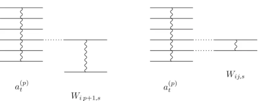
Fig. 4.1. Two terms of the productAN(at(p))AN(Ws), represented as labelled diagrams. A tree term (left)
produces a tree diagram. A loop term (right) produces a diagram with one loop
The mean-field limit is the limit n=νN → ∞, whereν >0 is some constant. The above estimate is clearly inadequate to prove statements about the mean-field limit. In order to obtain estimates uniform in N , more care is needed.
To see why the above estimate is so crude, consider the commutator iN 2 AN(Ws),AN(at(p)) H(n) ± = p! Np n p i NP± 1≤i<j≤n Wi j,s,a(tp)⊗1(n−p) P±.
We see that most terms of the commutator vanish (namely, whenever p<i< j ). Thus,
for large n, the above estimates are highly wasteful. This can be remedied by more careful bookkeeping. We split the commutator into two terms: the tree terms, defined by 1≤i ≤ p and p + 1≤ j ≤n, and the loop terms, defined by 1≤i < j ≤ p. All other
terms vanish. This splitting can also be inferred from (3.8).
The naming originates from a diagrammatic representation (see Fig. 4.1).
A p-particle operator is represented as a wiggly vertical line to which are attached
p horizontal branches on the left and p horizontal branches on the right. Each branch on
the left represents a creation operatorψ∗N(xi), and each branch on the right an annihila-tion operatorψN(yi). The productAN(a(p))AN(b(q))of two operators is given by the
sum over all possible pairings of the annihilation operators inAN(a(p))with the creation
operators inAN(b(q)). Such a contraction is graphically represented as a horizontal line
joining the corresponding branches. We consider diagrams that arise in this manner from the multiplication of a finite number of operators of the formAN(a(p)).
We now generalise this idea to a systematic scheme for the multiple commutators appearing in the Schwinger-Dyson expansion. To this end, we decompose the multiple commutator (iN)k 2k AN(Wtk), . . . AN(Wt1),AN(a (p) t ) . . .
into a sum of 2kterms obtained by writing out each commutator. Each resulting term is a product of k + 1 second-quantised operators, which we furthermore decompose into a sum over all possible contractions for which r >0 in (3.3) (at least one contraction for each multiplication). The restriction r >0 follows from[a(p),b(q)]0 =0. This is
We call the resulting terms elementary. The idea is to classify all elementary terms according to their number of loops l. Write
(iN)k 2k AN(Wtk), . . . AN(Wt1),AN(a (p) t ) . . .= k l=0 1 Nl AN Gt(k,t,1,...,l) tk(a(p)) , (4.4) where G(tk,t,1,...,l) tk(a
(p))is a(p +k−l)-particle operator, equal to the sum of all elementary
terms with l loops. It is defined through the recursion relation (onH(±p+k−l))
G(tk,t,1,...,l) tk(a(p))=i(p + k−l−1) Wtk,G(tk,t−1,...,1,l)tk−1(a (p)) 1 + i p + k−l 2 Wtk,G(t,kt−1,...,1,l−tk1−)1(a (p)) 2 =i P± p+k−l−1 i=1 Wi p+k−l,tk,G(tk,t−1,...,1,l)tk−1(a (p))⊗1 P± + i P± 1≤i<j≤p+k−l Wi j,tk,G (k−1,l−1) t,t1,...,tk−1(a (p))P±, (4.5) as well as G(t0,0)(a(p)):=a( p) t . If l <0, l>k, or p+k−l>n, then G( k,l) t,t1,...,tk(a(p))=0.
The interpretation of the recursion relation is simple: a(k,l)-term arises from either a
(k−1,l)-term without adding a loop or from a(k−1,l−1)-term to which a loop is added. It is not hard to see, using induction on k and the definition (4.5), that (4.4) holds. It is often convenient to have an explicit formula for the decomposition into elementary terms: G(tk,t,1,...,l) tk(a (p)) = c(p,k,l) α=1 G(tk,t,1,...,l)(α)tk(a (p)), where G(t,kt,1l,...,)(α)tk(a(
p))is an elementary term, and c(p,k,l)is the number of elementary
terms in G(t,kt,1,...,l) tk(a(p)).
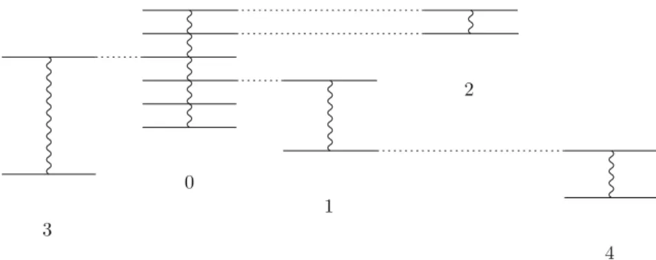
In order to establish a one-to-one correspondence between elementary terms and diagrams, we introduce a labelling scheme for diagrams. Consider an elementary term arising from a choice of contractions in the multiple commutator of order k, along with its diagram. We label all vertical lines v with an index iv ∈ Nas follows. The ver-tical line of a(p) is labelled by 0. The vertical line of the first (i.e. innermost in the multiple commutator) interaction operator is labelled by 1, of the second by 2, and so on (see Fig.4.2). Conversely, every elementary term is uniquely determined by its labelled diagram. We consequently useα =1, . . . ,c(p,k,l)to index either elementary terms or labelled diagrams.
Use the shorthand t=(t1, . . . ,tk)and define
G(tk,l)(a(p)) :=
k(t)
dt G(tk,t,l)(a(p)). (4.6)
Fig. 4.2. The labelled diagram corresponding to a one-loop elementary term in the commutator of order 4 eit HNAN(a(p))e−it HN = ∞ k=0 k l=0 1 Nl AN G(tk,l)(a(p)) , (4.7)
which converges in norm onH(±n), n∈N, for all times t.
5. Convergence for Bounded Interaction
For a bounded interaction potential,w∞ <∞, it is now straightforward to control the mean-field limit.
Lemma 5.1. We have the bound
G(tk,t,l)(a(p)) ≤ c(p,k,l)wk∞a(p). (5.1) Furthermore, c(p,k,l) ≤ 2k k l (p + k−l)l(p + k−1)· · ·p. (5.2)
Proof. Assume first that l =0. Then the number of labelled diagrams is clearly given by 2kp· · ·(p + k−1). Now if there are l loops, we may choose to add them at any l of the k steps when computing the multiple commutator. Furthermore, each addition of a loop produces at most p + k−l times more elementary terms than the addition of a tree
branch. Combining these observations, we arrive at the claimed bound for c(p,k,l). Alternatively, it is a simple exercise to show the claim, with c(p,k,l)replaced by the bound (5.2), by induction on k.
Lemma 5.2. Letν >0 and t < (8νw∞)−1. Then, onH(ν±N), the Schwinger-Dyson series (4.7) converges in norm, uniformly in N .
Proof. Recall that p + k−l ≤ n for nonvanishingAN
Gt(k,t,l)(a(p))
H(n)
± . Using the
symbol I{A}, defined as 1 if A is true and 0 if A is false, we find
∞ k=0 k l=0 1 Nl k(t)dt AN G(tk,t,l)(a(p)) H(νN) ± ≤∞ k=0 k l=0 (p + k−l)l Nl I{p+k−l≤νN} 1 k!(2w∞t) k k l p + k−1 k k!νp+k−la(p) ≤∞ k=0 (8νw∞t)k(2ν)pa(p) = 1 1−8νw∞t (2ν) p a(p),
where we used thatlk=0
k l
=2k, and in particularkl≤2k.
In the spirit of semi-classical expansions, we can rewrite the Schwinger-Dyson series to get a “1/N -expansion”, whereby all l-loop terms add up to an operator of order O(N−l).
Lemma 5.3. Let t< (8νw∞)−1and L∈N. Then we have onH(ν±N),
eit HNA N(a(p))e−it HN = L−1 l=0 1 Nl ∞ k=l AN G(tk,l)(a(p)) + O 1 NL ,
where the sum converges uniformly in N .
Proof. Instead of the full Schwinger-Dyson expansion (4.2), we can stop the expansion whenever L loops have been generated. More precisely, we iterate (4.1) and use (3.8) at each iteration to split the commutator into tree (r =1) and loop (r =2) terms. Whenever a term obtained in this fashion has accumulated L loops, we stop expanding and put it into a remainder term. Thus all fully expanded terms are precisely those arising from diagrams containing up to L−1 loops, and it is not hard to show that the remainder term is of order N−L.
In view of later applications, we also give a proof using the fully expanded Schwinger-Dyson series. From Lemma5.2we know that the sum converges onH(ν±N)in norm, uni-formly in N , and can be reordered as
eit HNAN(a(p))e−it HN = ∞ l=0 1 Nl ∞ k=l k(t) dt AN G(tk,t,l)(a(p)) ,
∞ l=L 1 Nl ∞ k=l k(t)dt AN G(tk,t,l)(a(p)) H(νN) ± ≤ 1 NL ∞ l=L ∞ k=l (p + k−l)l Nl−L I{p+k−l≤νN} ×1 k!(2w∞t) k k l p + k−1 k k!νp+k−la(p) ≤ 1 (νN)L ∞ l=L ∞ k=l (p + k−l)L(8νw∞t)k(2ν)pa(p) = 1 (νN)L ∞ l=L ∞ k=0 (p + k)L(8νw∞t)k+l(2ν)pa(p) ≤ (ν1 N)L ∞ l=L (8νw∞t)l e pL! (1−8νw∞t)L+1(2ν) pa(p) = 1 (νN)L epL!(8νw∞t)L (1−8νw∞t)L+2(2ν) p a(p),
where we used that∞k=0(p + k)Lxk ≤ (1−epxL)L+1! .
6. Convergence for Coulomb Interaction
In this section we consider an interaction potential of the form
w(x) = κ 1
|x|, (6.1)
whereκ∈R. We take the one-body Hamiltonian to be
h = −,
the nonrelativistic kinetic energy without external potentials. We assume this form of h andwthroughout Sects.6and7. In Sect.8, we discuss some generalisations.
6.1. Kato smoothing. The non-relativistic dispersive nature of the free time evolution
eitis essential for controlling singular potentials. The key tool for all of the following is the Kato smoothing estimate:
R
|x|−1eitψ2dt ≤ πψ2, (6.2)
whereψ∈L2(R3). Estimate (6.2) follows from Kato’s theory of smooth perturbations; see [20,23]. In Sect.8we provide a proof of (6.2) (without the sharp constantπ), for a larger class of interaction potentials, using Strichartz estimates.
In order to avoid tedious discussions of operator domains in equations such as (4.1), we introduce a cutoff to make the interaction potential bounded. Forε≥0 set
so thatwε∞≤ε−1. Now (6.2) implies, forε≥0, R wεeitψ2 dt ≤ R weitψ2dt ≤ πκ2ψ2. (6.3)
An immediate consequence is the following lemma. Lemma 6.1. Let(n)∈H±(n). Then
R Wε i je−it H0(n) 2 dt ≤ πκ 2 2 (n)2. (6.4)
Proof. By symmetry we may assume that(i,j)=(1,2). Choose centre of mass coordi-nates X :=(x1+x2)/2 andξ =x2−x1, set˜(n)(X, ξ,x3, . . . ,xn):=(n)(x1, . . . ,xn),
and write R Wε 12e− it H0(n)2dt = R wε(ξ)e2itξ˜(n)2 dt,
since H0 = −1−2 = −X/2−2ξ and[X, wε(ξ)] =0. Therefore, by (6.3)
and Fubini’s theorem, we find
R Wε 12e−it H0(n) 2 dt = d X dx3· · ·dxn dt dξwε(ξ)e2itξ˜(n)(X, ξ,x3, . . . ,xn)2 ≤ πκ2 2 d X dx3· · ·dxn dξ ˜(n)(X, ξ,x3, . . . ,xn)2 = πκ2 2 (n)2. By Cauchy-Schwarz we then find that
t 0 Wε i j,s( n) ds≤t1/2 R Wε i je− is H0(n)2ds 1/2 ≤ πκ2t 2 1/2 (n). (6.5) By iteration, this implies that, for all elementary termsα,
t 0 dt1. . . t 0 dtk G(tk,t,l)(α),ε(a(p))(p+k−l)≤ πκ2t 2 k/2 a(p) (p+k−l),(6.6) where the superscriptεreminds us that Gt(,kt,l)(α),ε(a(p))is computed with the regularised
potentialwε. Thus one finds
G(k,l),ε t (a(p)) ≤ c(p,k,l) πκ2t 2 k/2 a(p), for allε≥0.
Unfortunately, the above procedure does not recover the factor 1/k! arising from the time-integration over the k-simplexk(t), which is essential for our convergence
estimates. First iterating (6.4) and then using Cauchy-Schwarz yields a factor 1/√k!,
which is still not good enough.
A solution to this problem must circumvent the highly wasteful procedure of replac-ing the integral overk(t)with an integral over[0,t]k. The key observation is that, in the sum over all labelled diagrams, each diagram appears of the order of k!times with different labellings.
6.2. Graph counting. In order to make the above idea precise, we make use of graphs
(related to the above diagrams) to index terms in our expansion of the multiple commu-tator (iN)k 2k AN(Wtk), . . . AN(Wt1),AN(a (p) t ) . . .. (6.7)
The idea is to assign to each second quantised operator a vertexv =0, . . . ,k, and to
represent each creation and annihilation with an incident edge. A pairing of an annihila-tion operator with a creaannihila-tion operator is represented by joining the corresponding edges. The vertex 0 has 2 p edges and the vertices 1, . . . ,k have 4 edges. We call the vertex 0
the root.
The edges incident to each vertex v are labelled using a pairλ = (d,i), where
d =a,c is the direction (a stands for “annihilation” and c for “creation”) and i labels
edges of the same direction; i =1, . . . ,p ifv=0 and i =1,2 ifv =1, . . . ,k. Thus,
a labelled edge is of the form{(v1, λ1), (v2, λ2)}. GraphsGwith such labelled edges
are graphs over the vertex set V(G)= {(v, λ)}. We denote the set of edges of a graph
G(a set of unordered pairs of vertices in V(G)) by E(G). The degree of each(v, λ)is either 0 or 1; we call(v, λ)an empty edge ofv if its degree is 0. We often speak of connecting two empty edges, as well as removing a nonempty edge; the definitions are self-explanatory.
We may drop the edge labelling ofGto obtain a (multi)graphGover the vertex set {0, . . . ,k}: Each edge{(v1, λ1), (v2, λ2)} ∈E(G)gives rise to the edge{v1, v2} ∈E(G).
We understand a path inGto be a sequence of edges in E(G)such that two consecutive edges are adjacent in the graphG. This leads to the notions of connectedness ofGand loops inG.
The admissible graphs – i.e. graphs indexing a choice of pairings in the multiple commutator (6.7) – are generated by the following “growth process”. We start with the empty graphG0, i.e. E(G0)= ∅. In a first step, we choose one or two empty edges of 1 of
the same direction and connect each of them to an empty edge of 0 of opposite direction. Next, we choose one or two empty edges of 2 of the same direction and connect each of them to an empty edge of 0 or 1 of opposite direction. We continue in this manner for all vertices 3, . . . ,k. We summarise some key properties of admissible graphsG. (a) Gis connected.
(b) The degree of each(v, λ)is either 0 or 1.
(c) The labelled edge{(v1, λ1), (v2, λ2)} ∈ E(G)only ifλ1 andλ2 have opposite
directions.
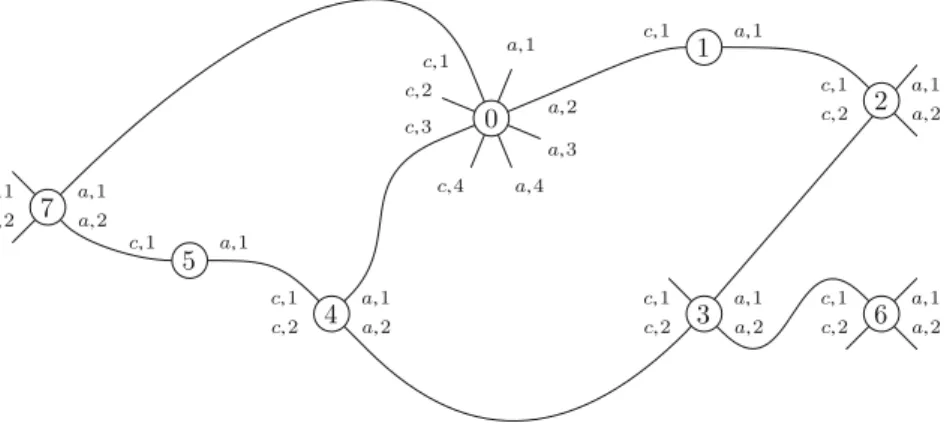
Property (c) implies that each graphGhas a canonical directed representative, where each edge is ordered from the a-label to the c-label. See Fig.6.1for an example of such a graph.
We call a graphGof type(p,k,l)whenever it is admissible and it contains l loops. We denote byG(p,k,l)the set of graphs of type(p,k,l).
Fig. 6.1. An admissible graph of type(p=4,k=7,l=3)
By definition of admissible graphs, each contraction in (6.7) corresponds to a unique admissible graph. A contraction consists of at least k and at most 2k pairings. A con-traction giving rise to a graph of type(p,k,l)has k + l pairings. The summand in (6.7) corresponding to any given l-loop contraction is given by an elementary term of the form
(iN)k 2kNk+lAN b(p+k−l) , (6.8)
where the(p + k−l)-particle operator b(p+k−l)is of the form
b(p+k−l)=P±Wi1j1,tv1· · ·Wirjr,tvr
at(p)⊗1(k−l)
Wir +1jr +1,tvr +1· · ·Wikjk,tvkP±, (6.9)
for some r =0, . . . ,k. Indeed, the (anti)commutation relations (A.2) imply that each pairing produces a factor of 1/N . Furthermore, the creation and annihilation operators of
each summand corresponding to any given contraction are (by definition) Wick ordered, and one readily sees that the associated integral kernel corresponds to an operator of the form (6.9). Thus we recover the splitting (4.4), whereby Gt(,kt,1,...,l) tk(a(p))is a sum,
indexed by all l-loop graphs, of elementary terms of the form (6.9).
As remarked above, we need to exploit the fact that many graphs have the same topo-logical structure, i.e. can be identified after some permutation of the labels{1, . . . ,k}of the vertices corresponding to interaction operators. We therefore define an equivalence relation on the set of graphs:G ∼G if and only if there exists a permutationσ ∈ Sk
such thatG=Rσ(G). Here Rσ(G)is the graph defined by
{(v1, λ1), (v2, λ2)} ∈ E(Rσ(G)) ⇐⇒ {(σ(v1), λ1), (σ(v2), λ2)} ∈E(G),
whereσ (0)≡0. We call equivalence classes[G]graph structures, and denote the set
of graph structures of admissible graphs of type(p,k,l)byQ(p,k,l).
Note that, in general, Rσ(G)need not be admissible ifGis admissible. It is conve-nient to increaseG(p,k,l)to include all Rσ(G), whereσ ∈ SkandGis admissible. In order to keep track of the admissible graphs in this larger set, we introduce the symbol
iG which is by definition 1 ifG ∈ G(p,k,l)is admissible and 0 otherwise. Because
Rσ(G)=Gifσ = id,
Our goal is to find an upper bound on the number of graph structures of type(p,k,l), which is sharp enough to show convergence of the Schwinger-Dyson series (4.2). Let us start with tree graphs: l =0. In this case the number of graph structures is equal to 2k times the number of ordered trees1with k + 1 vertices, whose root has at most 2 p children and whose other vertices have at most 3 children. The factor 2karises from the fact that each vertexv=1, . . . ,k can use either of the two empty edges of compatible
direction to connect to its parent. We thus need some basic facts about ordered trees, which are covered in the following (more or less standard) combinatorial digression.
For x,t ∈Rand n∈Ndefine
An(x,t) := x x + nt x + nt n (6.11) as well as A0(x,t):=1. After some juggling with binomial coefficients one finds
n
k=0
Ak(x,t)An−k(y,t) = An(x + y,t); (6.12)
see [12] for details. Therefore
n1+···+nr=n An1(x1,t)· · ·Anr(xr,t) = An(x1+· · ·+ xr,t). (6.13) Set Cmn := An(1,m) = 1 1 + nm 1 + nm n = 1 n(m−1)+ 1 nm n , (6.14)
the nthm-ary Catalan number. Thus we have
n1+···+nr=n Cnm1· · ·C m nr = r r + nm r + nm n . (6.15) In particular, n1+···+nm=n−1 Cnm1· · ·Cnmm = Cnm. (6.16) Define an m-tree to be an ordered tree such that each vertex has at most m children. The number of m-trees with n vertices is equal to Cnm. This follows immediately from
Cm0 =1 and from (6.16), which expresses that all trees of order n are obtained by adding
m (possibly empty) subtrees of combined order n−1 to the root.
We may now compute|Q(p,k,0)|. Since the root of the tree has at most 2 p children, we may express|Q(p,k,0)|as the number of ordered forests comprising 2 p (possibly empty) 3-trees whose combined order is equal to k. Therefore, by (6.15),
|Q(p,k,0)| = 2k n1+···+n2 p=k Cn31· · ·Cn32 p = 2k 2 p 2 p + 3k 2 p + 3k k . (6.17)
Next, we extend this result to all values of l in the form of an upper bound on |Q(p,k,l)|.
Lemma 6.2. Let p,k,l∈N. Then |Q(p,k,l)| ≤ 2k k l 2 p + 3k k (p + k−l)l. (6.18)
Proof. The idea is to remove edges fromG∈G(p,k,l)to obtain a tree graph, and then use the special case (6.17).
In addition to the properties (a) – (c) above, we need the following property of
G(p,k,l):
(d) IfG∈G(p,k,l)then there exists a subsetV⊂ {1, . . . ,k}of size l and a choice of directionδ:V → {a,c}such that, for eachv ∈V, both edges ofvwith direction
δ(v) are nonempty. Denote byE(v) ⊂ E(G)the set consisting of the two above edges. We additionally require that removing one of the two edges of E(v)from
G, for eachv ∈V, yields a tree graph, with the property that, for eachv ∈V, the remaining edge ofE(v)is contained in the unique path connectingvto the root. This is an immediate consequence of the growth process for admissible graphs. The setV corresponds to the set of vertices whose addition produces two edges. Note that property (d) is independent of the representative and consequently holds also for non-admissible
G∈G(p,k,l).
Before coming to our main argument, we note that a tree graphT ∈G(p,k,0)gives rise to a natural lexicographical order on the vertex set{1, . . . ,k}. Letv ∈ {1, . . . ,k}.
There is a unique path that connectsvto the root. Denote by 0=v1, v2, . . . , vq =vthe
sequence of vertices along this path. For each j=1, . . . ,q−1, letλjbe the label of the
edge{vj, vj +1}atvj. We assign tovthe string S(v):=(λ1, . . . , λq−1). Choose some
(fixed) ordering of the sets of labels{λ}, for eachv. Then the set of vertices{1, . . . ,k}
is ordered according to the lexicographical order of the string S(v).
We now start removing loops from a given graphG ∈G(p,k,l). DefineR1as the
graph obtained fromGby removing all edges inv∈VE(v). By property (d) above,R1
is a forest comprising l trees. DefineT1as the connected component ofR1containing
the root. Now we claim that there is at least onev ∈ V such that both edges ofE(v) are incident to a vertex ofT1. Indeed, were this not the case, we could choose for each
v∈Van edge inE(v)that is not incident to any vertex ofT1. CallR1the graph obtained
by adding all such edges toR1. Now, since no vertex inVis in the connected
compo-nent ofR1, it follows that no vertex inVis in the connected componentR1. This is a
contradiction to property (d) which requires thatR1should be a (connected) tree. Let us therefore consider the setV˜ of all v ∈ V such that both edges ofE(v)are incident to a vertex ofT1. We have shown thatV˜ = ∅. For each choice ofvand e, where
v ∈ ˜V and e∈ E(v), we get a forest of l−1 trees by adding e to the edge set ofR1.
Thenvis in the same tree as the root, so that each such choice ofvand e yields a string
S(v)as described above. We choosev1and e(v1)as the unique couple that yields the
smallest string (note that different choices have different strings). Finally, setG1equal
toGfrom which e(v1)has been removed, andV1:=V\ {v}.
We have thus obtained an(l−1)-loop graphG1and a setV1of size l−1, which
together satisfy the property (d). We may therefore repeat the above procedure. In this manner we obtain the sequencesv1, . . . , vlandG1, . . . ,Gl. Note thatGl is obtained by
removing the edges e(v1), . . . ,e(vl)fromG, and is consequently a tree graph. Also, by
construction, the sequencev1, . . . , vlis increasing in the lexicographical order ofGl.
Next, consider the tree graphGl. Each edge e(vj)connects the single empty edge of
vis smaller thanvj in the lexicographical order ofGl. It is easy to see that, for each j ,
there are at most(p + k−l)such connections.
We have thus shown that we can obtain anyG ∈ G(p,k,l)by choosing some tree
Gl ∈G(p,k,0), choosing l elementsvj out of{1, . . . ,k}, ordering them
lexicograph-ically (according to the order ofGl) and choosing an edge out of at most(p + k−l)
possibilities forv1, . . . , vl. Thus,
G(p,k,l) ≤ k l
(p + k−l)lG(p,k,0). The claim then follows from (6.10) and (6.17).
6.3. Proof of convergence. We are now armed with everything we need in order to
estimatek(t)dt G( k,l) t,t (a(p)). Recall that G(t,kt,1,...,l) tk(a(p)) = ik 2k G∈G(p,k,l) iGGt(,kt,1,...,l)(Gtk)(a(p)), (6.19) where G(t,kt,1,...,l)(Gt)k(a(
p))is an elementary term of the form (6.9) indexed by the graphG.
We rewrite this using graph structures. Pick some choiceP :Q(p,k,l)→G(p,k,l)
of representatives. Then we get
G(tk,t,1,...,l) tk(a (p))= ik 2k Q∈Q(p,k,l) G∈Q iGG(tk,t,1,...,l)(Gt)k(a (p)) = ik 2k Q∈Q(p,k,l) σ∈Sk iRσ(P(Q))G(tk,t,1,...,l)(Rtσk(P(Q)))(a (p)).
Now, by definition of Rσ, we see that
G(tk,t,1,...,l)(Rtσk(G))(a (p)) = Gt(k,t,σ(l)(1)G,...,) tσ (k)(a( p)). Thus, k(t)dt G (k,l) t,t1,...,tk(a (p))= ik 2k Q∈Q(p,k,l) σ∈Sk iRσ(P(Q)) k(t)dt G (k,l)(P(Q)) t,tσ(1),...,tσ (k)(a (p)) = ik 2k Q∈Q(p,k,l) k Q(t) dt G(t,kt,1,...,l)(Ptk(Q))(a(p)), where k Q(t):= {(t1, . . . ,tk): ∃σ ∈Sk :iRσ(P(Q)) =1, (tσ(1), . . . ,tσ(k))∈k(t)} ⊂ [0,t]k
Therefore, (6.5) and (6.9) imply, for any(p+k−l)∈H±(p+k−l), that k(t)dt G (k,l) t,t (a(p)) (p+k−l) ≤ 1 2k Q∈Q(p,k,l) k Q(t) dtG(tk,t,1,...,l)(Pt(kQ))(a (p)) (p+k−l) ≤ 1 2k Q∈Q(p,k,l) [0,t]kdt G(k,l)(P(Q)) t,t1,...,tk (a (p)) (p+k−l) ≤ 1 2k Q∈Q(p,k,l) πκ2t 2 k/2 a(p)(p+k−l) ≤ 2 p + 3k k k l (p + k−l)l πκ2t 2 k/2 a(p)(p+k−l),
where the last inequality follows from Lemma 6.2. Of course, the above treatment remains valid for regularised potentials. We summarise:
G(tk,l),ε(a(p)) ≤ 2 p + 3k k k l (p + k−l)l πκ2t 2 k/2 a(p), (6.20) for allε≥0.
Using (6.20) we may now proceed exactly as in the case of a bounded interaction potential. Let
ρ(κ, ν) := 1
128πκ2ν2. (6.21)
The removal of the cutoff and summary of the results are contained in Lemma 6.3. Let t< ρ(κ, ν). Then we have onH(ν±N)
eit HNA N(a(p))e−it HN = ∞ k=0 k l=0 1 Nl AN G(tk,l)(a(p)) , (6.22)
in operator norm, uniformly in N . Furthermore, for L ∈N, we have the 1/N -expansion
eit HNAN(a(p))e−it HN = L−1 l=0 1 Nl ∞ k=l AN G(tk,l)(a(p)) + O 1 NL , (6.23)
where the sum converges onH(ν±N)uniformly in N .
Proof. Using (6.20) we may repeat the proof of Lemma5.3to the letter to prove the statements about convergence. Thus (6.22) holds for allε >0. The proof of (6.22) for
ε=0 follows by approximation and is banished to AppendixB.
7. Mean-Field Limit
In this section we identify the mean-field dynamics as the dynamics given by the Hartree equation.
7.1. Hartree equation. The Hartree equation reads
i∂tψ = hψ+(w∗ |ψ|2)ψ. (7.1)
It is the equation of motion of a classical Hamiltonian system with phase space :=
H1(R3). Here H1(R3)is the usual Sobolev space of index one. In analogy toAN we
define A as the map from closed operators onH+(p)to functions on phase space, through
A(a(p))(ψ):= ψ⊗p,a(p)ψ⊗p = dx1· · ·dxpdy1· · ·dypψ(¯ xp)· · · ¯ ψ(x1)a(p)(x1, . . . ,xp;y1, . . . ,yp) ψ(y1)· · ·ψ(yp).
We define the space of “observables”Aas the linear hull of{A(a(p)) : p∈N,a(p)∈B
(H(p) + )}.
The Hamilton function is given by
H := A(h)+1 2A(W), i.e. H(ψ)= dx|∇ψ|2+ 1 2 dx(w∗ |ψ|2)|ψ|2=ψ ,hψ+1 2ψ ⊗2, Wψ⊗2. (7.2) Using the Hardy-Littlewood-Sobolev and Sobolev inequalities (see e.g. [13]) one sees that H(ψ)is well-defined on: dx dy |ψ(x)| 2|ψ(y)|2 |x−y| |ψ| 22 6/5 = ψ 4 12/5 ψ 4 H1,
where the symbol means the left side is bounded by the right side multiplied by a positive constant that is independent ofψ.
The Hartree equation is equivalent to
i∂tψ = ∂ψ¯H(ψ).
The symplectic form onis given by
ω=i
dx dψ(¯ x)∧dψ(x),
which induces a Poisson bracket given by
{ψ(x),ψ(¯ y)} = iδ(x−y), {ψ(x), ψ(y)} = { ¯ψ(x),ψ(¯ y)} = 0. For A,B ∈Awe have that
{A,B}(ψ) = i
dx∂ψA(ψ) ∂ψ¯B(ψ)−∂ψB(ψ) ∂ψ¯A(ψ).
The “mass” function
N(ψ) :=
dx|ψ|2
is the generator of the gauge transformationsψ→e−iθψ. By the gauge invariance of the Hamiltonian,{H,N} = 0, we conclude, at least formally, that N is a conserved quantity. Similarly, the energy H is formally conserved.
(i) A(a(p))=A(a(p))∗.
(ii) If a(p)∈B(H(+p))and b∈B(H), then
A(a(p))(bψ) = A
(b∗)⊗pa(p)b⊗p
(ψ).
(iii) If a(p)and b(q)are p- and q-particle operators, respectively, then
A(a(p)),A(b(q)) = i pqAa(p),b(q)1 . (7.3) (iv) If a(p)∈B(H(+p)), then A(a(p))(ψ) ≤ a(p) ψ2 p. (7.4)
The free time evolution
φt
0(ψ) := e−it hψ
is the Hamiltonian flow corresponding to the free Hamilton function A(h). We abbrevi-ate the free time evolution of observables A∈Aby At := A◦φ0t. Thus, A(a(p))t =
A(at(p)).
In order to define the Hamiltonian flow on all of L2(R3), we rewrite the Hartree equation (7.1) with initial dataψ(0)=ψas an integral equation
ψ(t) = e−it hψ−i
t
0
ds e−i(t−s)h(w∗ |ψ(s)|2)ψ(s). (7.5) Lemma 7.1. Let ψ ∈ L2(R3). Then (7.5) has a unique global solution ψ(·) ∈ C
(R;L2(R3)), which depends continuously on the initial dataψ. Furthermore,ψ(t) =
ψ for all t . Finally, we have a Schwinger-Dyson expansion for observables: Let a(p)∈B(H(+p)),ν >0 and t< ρ(κ, ν). Then A(a(p))(ψ(t))= ∞ k=0 A G(tk,0)(a(p)) (ψ) =∞ k=0 1 2k k(t)dt A(Wtk), . . .A(Wt1),A(a (p) t ) . . .(ψ), (7.6)
uniformly in the ball Bν := {ψ∈ L2(R3) : ψ2≤ν}.
Proof. The well-posedness of (7.5) is a well-known result; see for instance [4,24]. The remaining statements follow from a “tree expansion”, which also yields an existence result. We first use the Schwinger-Dyson expansion to construct an evolution on the space of observables. We then show that this evolution stems from a Hamiltonian flow that satisfies the Hartree equation (7.5).
First, we generalise our class of “observables” to functions that are not gauge invari-ant, i.e. that correspond to bounded operators a(q,p) ∈ B(H+p;H
q
+). We set A(a(q,p))
(ψ):= ψ⊗q,a(q,p)ψ⊗p, and denote byAthe linear hull of observables of the form
A(a(q,p))with a(q,p) ∈B(H+p;H q +).
It is convenient to introduce the abbreviations
G := {A(h),· }, D := 1
2{A(W),· }.
Then eGt is well-defined onAthrough(eGtA)(ψ)= A(e−ihψ), where A ∈ A. Note also that
Ds := eGsDe−Gs = 1
2{A(Ws),· }.
Let A ∈ A. We use the Schwinger-Dyson series for e(G+D)t to define the flow S(t)A
through S(t)A:= ∞ k=0 k(t) dt Dtk· · ·Dt1e GtA = ∞ k=0 k(t) dt 1 2k A(Wtk), . . .A(Wt1),At). . .. (7.7) Our first task is to show convergence of (7.7) for small times.
Let A=A(a(q,p)). As with (7.3) one finds, after short computation, that 1 2{A(W),A(a (q,p))} = A i q i=1 Wi q+1(a(q,p)⊗1)−i p i=1 (a(q,p)⊗1)Wi p+1 .(7.8) Thus we see that the nested Poisson brackets in (7.7) yield a “tree expansion” which may be described as follows. Define Tt(,kt1),...,tk(a
(q,p))recursively through Tt(0)(a(q,p)):=a( q,p) t , Tt(,kt1,...,) tk(a (q,p)):= i P+ q+k−1 i=1 Wi q+k,tk Tt(,kt1,...,−1)tk−1(a (q,p))⊗1 P+ −i P+ p+k−1 i=1 Tt(,kt1,...,−1)tk−1(a (q,p))⊗1Wi p+k ,tkP+. Note that Tt(,kt1,...,) tk(a( q,p))is an operator fromH(p+k) + toH( q+k) + . Moreover, (7.8) implies that 1 2k A(Wtk), . . . A(Wt1),A(a (q,p) t ) . . . = A Tt(,kt1,...,) tk(a(q,p)) . (7.9)
Also, by definition, we see that for gauge-invariant observables a(p)we have
Tt(,kt1,...,) tk(a
(p)) = G(k,0) t,t1,...,tk(a
(p)).
We may use the methods of Sect. 6 to obtain the desired estimate. One sees that
Tt(,kt1),...,tk(a(
root has degree at most p + q, and whose other vertices have at most 3 children. From (6.15) we find that there are
p + q p + q + 3k p + q + 3k k
unlabelled trees of this kind. Proceeding exactly as in Sect.6we find that
k(t)dt Tt(,kt1,...,) tk(a(q,p))(p+k) ≤ p + q + 3k k πκ2t 2 k/2 a(q,p)(p+k),
where (p+k) ∈ H+(p+k). Letψ ∈ L2(R3)withψ2 ≤ ν. Then|A(a(q,p))(ψ)| ≤
a(q,p)ψp+q implies k(t)dt 21k A(Wtk), . . .A(Wt1),A(a (q,p) t ) . . .(ψ) ≤ p + q + 3k k πκ2t 2 k/2 a(q,p)νk+(p+q)/2. (7.10) Convergence of the Schwinger-Dyson series (7.7) for small times t follows immediately. Thus, for small times t, the flow S(t)is well-defined onA, and it is easy to check that it satisfies the equation
S(t)A = eGtA +
t
0
ds S(s)D eG(t−s)A, (7.11)
for all A∈A.
In order to establish a link with the Hartree equation (7.5), we consider f ∈ L2(R3)
and define the function Ff ∈ Athrough Ff(ψ) := f, ψ. Clearly, the mapping f →(S(t)Ff)(ψ)is antilinear and (7.10) implies that it is bounded. Thus there exists
a unique vectorψ(t)such that
(S(t)Ff)(ψ) =: f, ψ(t).
We now proceed to show that(S(t)A)(ψ)= A(ψ(t))for all A∈A. By definition, this is true for A=Ff. As a first step, we show that
S(t)(A B) = (S(t)A)(S(t)B), (7.12) where A,B∈A. Write S(t)(A B)= ∞ k=0 k(t)dt Dtk· · ·Dt1e Gt( A B) =∞ k=0 k(t)dt Dtk· · ·Dt1(AtBt),
where we used eGt(A B)=(eGtA)(eGtB). We now claim that
k(t)dt Dtk· · ·Dt1(AtBt)= l+m=k l(t)dt m(t)ds Dtl· · ·Dt1At Dsm· · ·Ds1Bt , (7.13)