Doctoral Dissertations Student Scholarship
Fall 2016
Computationally Efficient Specifications of Spatial
Point Process Models and Spatio-Temporal
Gaussian Models: Combining Remote Sensing
Drivers with Geospatial Disease Case Data to
Enhance Geographic Epidemiology
Beth Louise Ziniti
University of New Hampshire, Durham
Follow this and additional works at:https://scholars.unh.edu/dissertation
This Dissertation is brought to you for free and open access by the Student Scholarship at University of New Hampshire Scholars' Repository. It has been accepted for inclusion in Doctoral Dissertations by an authorized administrator of University of New Hampshire Scholars' Repository. For more information, please [email protected].
Recommended Citation
Ziniti, Beth Louise, "Computationally Efficient Specifications of Spatial Point Process Models and Spatio-Temporal Gaussian Models: Combining Remote Sensing Drivers with Geospatial Disease Case Data to Enhance Geographic Epidemiology" (2016).Doctoral Dissertations. 1378.
COMPUTATIONALLY EFFICIENT SPECIFICATIONS OF SPATIAL POINT PROCESS MODELS AND SPATIO-TEMPORAL GAUSSIAN MODELS: COMBINING REMOTE
SENSING DRIVERS WITH GEOSPATIAL DISEASE CASE DATA TO ENHANCE GEOGRAPHIC EPIDEMIOLOGY
BY
BETH L. ZINITI
B.A., McGill University, Quebec Canada, 2005 M.S., University of New Hampshire, 2012
DISSERTATION
Submitted to the University of New Hampshire in Partial Fulfillment of
the Requirements for the Degree of
Doctor of Philosophy in
Statistics
This dissertation has been examined and approved in partial fulfillment of the requirements for the degree of Ph.D. in Statistics by:
Dissertation Director, Dr. Ernst Linder, Professor of Mathematics & Statistics
Dr. Linyuan Li,
Professor of Mathematics & Statistics
Dr. Haiying Wang,
Assistant Professor of Mathematics & Statistics
Dr. Mark Lyon,
Associate Professor of Mathematics & Statistics
Dr. Nathan Torbick,
Director, Human & Environment Interactions Applied Geosolutions, LLC
On August 9 2016
DEDICATION
ACKNOWLEDGEMENTS
This dissertation could not have been written without the support and guidance from many individuals, and I would like to express my deepest appreciation to some of these people in particular.
To begin, I would like to give special thanks to my advisor, Dr. Ernst Linder, for
introducing me to Spatial Statistics and the EAR model, and for all his time and guidance that he has provided me in the research and writing of this dissertation. I was glad to revisit the topic of Markov Chains, which I first saw during my undergraduate studies and most enjoyed.
I would also like to thank the members of my committee Drs. Linyuan Li, Haiying Wang, Mark Lyon and Nathan Torbick for taking the time to discuss relevant research topics with me and to provide me useful suggestions and valuable comments.
I would like to give particular thanks to Dr. Nathan Torbick for introducing me to such an important and complex scientific application, as well as for providing all the water quality data and much guidance and suggestions in my modeling. Also I am thankful to all the employees of Applied Geosolutions for providing such a friendly and welcoming atmosphere, and especially to Megan Corbiere for all her work in processing the data.
I am thankful to all the people in the Dartmouth group in particular, Dr. Elijah Stommel, Dr. Angeline Andrew, Dr. Xun Shi, Dr. Tracie Caller and Ms. Patricia Henegan for providing the case data, for their interest in this work, and for all their helpful suggestions and comments.
The work in this dissertation was funded from the National Science Foundation grant GSS (BCS-1433756) and is part of a larger collaborative project that includes researchers from the University of New Hampshire, Applied Geosolutions LLC, Dartmouth College and the Dartmouth Hitchcock Medical Center. I am honored to have been a part of this project.
I am very grateful for the generous financial support I received during my doctorial studies and that allowed me to complete this dissertation. I would like to thank the UNH Mathematics and Statistics Department for providing me funding in the form of teaching assistantships as well as for funding to attend conferences. I would like to thank the UNH Graduate School for also providing funding to attend conferences. I am thankful for some additional funding I received as a consultant in the UNH Mathematics and Statistics
department’s statistical consulting service, in particular for a project requested by Senior Vice Provost for Research Jan Nesbit. I am thankful for the LandScan background population data paid for by the UNH Library.
I would like to thank Professor Edward Hinson and Professor Rita Hibschweiler for their guidance during my time at UNH, and to thank Jan Jankowski, Ellen O'Keefe, and April Flore in the math office for their various forms of support. I am thankful for the writing and editing assistance I received at the UNH writing center, in particular from Lauren Short and Molly Tetreault. I am grateful to my fellow graduate students; Meng Zhao, Michael Willliams, Shuang Wu, and many more for their many helpful and interesting conversations and for joining me on many hiking, running and x-country skiing adventures.
Finally, I am most grateful for my supportive and understanding family, especially thank you to my husband, Charlie Ziniti who has helped me through some difficult days, and to my father, Bill Roberts, for all his support, for his patience and for his persistence. I have finally found that something technical that I truly enjoy.
TABLE OF CONTENTS
DEDICATION ... iii
ACKNOWLEDGEMENTS ... iv
TABLE OF CONTENTS ... vi
LIST OF TABLES ... viii
LIST OF FIGURES ... ix
ABSTRACT ... xii
CHAPTER PAGE I INTRODUCTION ... 1
ALS IN NORTHERN NEW ENGLAND... 3
STUDY GOALS ... 5
II BASICS OF EPIDEMIOLOGY ... 10
2.1 TERMINOLOGY ... 10
2.2 ALSEXPECTED COUNTS ... 14
III DESCRIPTION OF ALS CASE AND EXPOSURE DATA ... 22
3.1 NNEALSCASE DATA ... 22
3.2 EXPOSURE METRICS FOR WATER QUALITY ... 23
3.2.1 Torbick et al. (2014) Water Quality Metrics ... 24
3.2.2 Phycocyanin (PC) Metric ... 26
3.2.3 Tropic Status Index (TSI) Metric ... 28
3.2.4 Lake Champlain Surface Water Temperatures ... 32
IV STATISTICAL MODELS ... 37
4.1 BAYESIAN INFERENCE FOR HIERARCHICAL MODELS ... 37
4.2 INTRODUCTION TO GAUSSIAN PROCESSES ... 44
4.3 COMPUTATIONAL EFFICIENCY ISSUES ... 49
4.4 GAUSSIAN MARKOV RANDOM FIELDS FOR SMOOTH PROCESSES ... 51
V SUMMARIZING DATA TO COMPUTATIONAL GRIDS ... 60
5.1 COMPUTATIONAL GRIDS FOR ESTIMATING ALSRISK ... 60
5.1.2 VTNH and VTNH_rmcty 4 and 8km Computational Grids ... 67
5.2 COMPUTATIONAL GRIDS FOR LAKE CHAMPLAIN SURFACE WATER TEMPERATURES ... 70
VI SPATIAL DISTRIBUTION OF ALS ... 73
6.1 GOALS & ORGANIZATION ... 73
6.2 MODEL... 74
6.3 ALSSPATIAL DISTRIBUTION IN NNE ... 76
6.4 ALSSPATIAL DISTRIBUTION IN VTNH VS VTNH_RMCTY ... 77
VII ESTIMATING EXPOSURE EFFECTS ... 82
7.1 RELATIONSHIP OF WATER QUALITY TO ALSRISK OVER NNE ... 83
7.1.1 Model ... 83
7.1.2 Results ... 84
7.2 RELATIONSHIP OF WATER QUALITY TO ALSRISK OVER VTNH AND VTNH_RMCTY ... 87
7.2.1 Model ... 87
7.2.2 Results ... 88
VIII EXPOSURE MODELING... 96
8.1 SPATIAL DISTRIBUTION OF HUC12MAX PC IN VT AND NH ... 96
8.2 SPATIO-TEMPORAL SURFACE TEMPERATURES OF LAKE CHAMPLAIN ... 99
8.2.1 Model ... 99
8.2.2 Results & Discussion ... 103
IX CONCLUSIONS... 110
X FUTURE WORK ... 114
REFERENCES ... 117
APPENDIX A: R CODE FOR CHAMPLAIN ANALYSIS ... 123
LIST OF TABLES
Table II-1. Observed ALS case counts by age/sex class and boundary area ... 16
Table II-2. Modified observed ALS case counts by age/sex class and boundary area ... 17
Table II-3. Comparison of total population counts by age/sex class for all of NNE ... 20
Table V-1. Minimum contrast estimates of the scale and variance parameters for the exponential covariance ... 62
Table V-2. Age/sex class case and population counts ... 64
Table V-3. Lattice cell frequency by ALS case count ... 65
Table V-4. Aggregation Scales used to summarize PC in ug/L & Lake TSI ... 69
Table VI-1. Number of lattice cells by boundary region and lattice resolution ... 75
Table VII-1. Summary of parameter posterior samples for BYM and Leroux models fit using CARBayes package in R with 1 chain having 1000 samples ... 84
Table VII-2. Odds Ratios (OR) of average Chl-A effect on ALS risk based on BYM and Leroux models ... 85
Table VII-3: Summary of P-values for each variables 16 models ... 89
Table VII-4. Marginal Posterior summaries of the coefficients for the 16 models that included PC IDW6 ... 92
Table VII-5. Odds ratio of effect of PC IDW 6 when model includes BYM random effects, SEDAC expected counts, the boundary is VTNH_rmcty, and the grid resolution is 8km ... 92
Table VII-6. Marginal Posterior summaries of the coefficients for the 16 models that included TSI_2004_IDW6... 93
Table VIII-1. Summary of posterior samples for model parameters (2160m grid) ... 104
LIST OF FIGURES
Figure II-1. Boundary areas of the study region are in gray; NNE (right); VTNH (middle); VTNH_rmcty (left). ... 14 Figure III-1. Distribution of lake average SD, TN and Chl-a satellite derived metrics for all 4453
lakes in NNE greater than 6 hectares. Top: Metric boxplots of all lakes; Bottom: Metric histogram of non-outliers values only... 25 Figure III-2. Late Summer 2009/2010 snapshot values of lake average secchi depth, total
nitrogen, and chlorophyll-a for lakes sized 6 hectares for more across Northern New
England ... 26 Figure III-3. Late Summer 2014/2015 Snapshot Representation of the amount of phycocyanin for
each 30m water pixel for all lakes sized 6 hectares or more in Northern NewEngland ... 27 Figure III-4. Lake average phycocyanin (ug/L) for 4867 lakes sized 6 hectares or more across
Northern New England based on Landsat derived metric at 30 meter resolution pixels. ... 28 Figure III-5. JAS 2000-2005 TSI lake classifications compared with the early period 2000-2001
classification, the middle period 2002-2003 classification and the late period 2004-2005 classification. ... 30 Figure III-6. Number of 50% cloud free Landsat overpasses by lake for each time period ... 31 Figure III-7. Average time of month for all 50% cloud free Landsat overpass dates by lake for
each time period. ... 32 Figure III-8. Sampling Pattern of Landsat LT5 and LE7 for mostly cloud free images of path row tile 014029 over Lake Champlain ... 34 Figure III-9. Average lake satellite-derived surface water temperatures of Lake Champlain from
1984-2014 by day of year ... 35 Figure III-10. Satellite-derived surface water temperatures of Lake Champlain from 1984-2011
for days of year 195 to 244 vs. buoy in-situ water temperatures from 1992-2013 for days of year 195 to 244 and depths below 4 meters. (Gray line at 16 degrees Celsius.) ... 35 Figure III-11. Satellite-derived surface water temperatures of Lake Champlain and Landsat
image near St. Albans Bay for Year 1989 and Day of Year 230 ... 36 Figure IV-1. Eigenvalues and Eigenvectors of EAR’s precision matrix Q compared with Spatial
Regression Covariates ... 58 Figure IV-2. Simulated EAR process with mean 0 and 𝜓 = 0.5 for different values of 𝜃 ... 59 Figure V-1. Illustration of direction aggregation effect (colors red, brown, green, blue, orange,
Figure V-2. NNE region overlaid with 8km resolution lattice (black cells are 13 excluded cells) ... 67 Figure V-3. Semivariance plots for each least squares estimated parameter ... 72 Figure V-4. Computational Grids used to model remotely sensed surface water temperatures of
Lake Champlain ... 72 Figure VI-1. Fixed modeling component combinations used in estimation of ALS spatial
distribution ... 73 Figure VI-2. Posterior relative risk mean estimates... 76 Figure VI-3. Probability Relative Risk is greater than 1.5 for VTNH by resolution scale and
background population... 78 Figure VI-4. Probability Relative Risk is greater than 1.5 for VTNH_rmcty using SEDAC by
resolution scale; (left) 4km and (right) 8km ... 80 Figure VI-5. Comparison of DIC values between the 8 models estimating the spatial distribution
of ALS using different population backgrounds, different boundaries and different
computational grid size resolutions. ... 81 Figure VII-1. Illustration of direction Effect ... 86 Figure VII-2. Illustration showing the different fixed components of the model that are varied . 88 Figure VII-3. Distribution of p-values for all 320 models ... 90 Figure VII-4. Boxplots (distributions) of 16 p-values for each of the 20 variables ... 91 Figure VII-5. Distribution of lake TSI 2004-2005 temporal aggregation; left is original lake
aggregation scale; upper right is the histogram of TSI 2004-2005 values when aggregated to match 4km grid using IDW6 scale; lower right is the spatial distribution of the histogram values. ... 94 Figure VII-6. Comparison of DIC values between the 320 models estimating the effect of water
metric regression variables on the spatial distribution of ALS using different population backgrounds, different boundaries, different computational grid size resolutions, different water metrics and using BYM or no spatial random effects. ... 95 Figure VIII-1. HUC12 boundaries colored by Max lake average PC in ug/L (White areas do not
contain any lakes sized a least 6 hectares.) ... 97 Figure VIII-2. Model predicted MaxPC_huc12 (left); Lower 95% credibility bound (middle);
Upper 95% credibility bound (right)... 98 Figure VIII-3. Proportion of posterior spatial random effect samples greater than 0. ... 99 Figure VIII-4. Eigenvalues by ID for the matrix D-A when the 1080m lattice is used. ... 101
Figure VIII-5.Example Eigenvectors of the Matrix D – A for the 1080m computational lattice. (Top: Large-scale spatial variability; Bottom: Small-scale spatial variability). ... 102 Figure VIII-6. Posterior Mean of Average Surface water temperatures (right) and 95% credibility
interval (center and left) based on the 1080m resolution grid. ... 105 Figure VIII-7. Locations of significantly warmer and significantly cooler than lake average
surface water temperatures. ... 106 Figure VIII-8. Satellite-derived surface water temperatures of Lake Champlain and Landsat
image near Missiquoi Bay for Year 2008 and Day of Year 227 ... 107 Figure VIII-9. Posterior Mean of Temperature Trends (right) and 95% credibility interval (center and left) based on the 1080m resolution grid... 108 Figure VIII-10. Locations with significantly warmer or cooler temperatures based on a p-value of
0.05 and confidence interval of 95% ... 108 Figure VIII-11. Probability of increasing trends ... 109
ABSTRACT
COMPUTATIONALLY EFFICIENT SPECIFICATIONS OF SPATIAL POINT PROCESS MODELS AND SPATIO-TEMPORAL GAUSSIAN MODELS: COMBINING REMOTE
SENSING DRIVERS WITH GEOSPATIAL DISEASE CASE DATA TO ENHANCE GEOGRAPHIC EPIDEMIOLOGY
by Beth L. Ziniti
University of New Hampshire, September, 2016
In this dissertation, the flexibility of Bayesian hierarchical models specified using a latent Gaussian Markov Random Field (GMRF) are evaluated for use in analyzing large complex spatial and spatio-temporal data with the goal of contributing to an interdisciplinary effort of developing an eco-epidemiological model that quantifies the relationship between remotely sensed water quality and the incidence of ALS (Amyotrophic Lateral Sclerosis or Lou Gehrig’s Disease) over large areas such as Northern New England (NNE).
In particular, a Log-Gaussian Cox Process (LGCP) specified by the logarithm of a GMRF on a regular lattice is shown to allow for simultaneous estimation of the spatial distribution of ALS risk and its relationship to remotely sensed water quality metrics. This approach improves
on previous analyses of the dataset considered by explicitly accounting for the spatial uncertainty in determining locations of ALS “hotspots” needed in the estimation of the hotspots’ relationship to the water quality of lakes in NNE.
Finally, since warming lake temperatures have been associated with more frequent cyanobacteria blooms (blue-green algae), which is a possible risk factor of ALS, a spatially varying coefficient model specified with an Extended Autoregression (EAR) latent process is used in an analysis of remotely sensed surface water temperatures of Lake Champlain. New interpretations of the EAR model are suggested and issues relating to its parameter’s
I INTRODUCTION
The field of eco-epidemiology seeks to identify causes of spatial and temporal patterns in disease incidence and mortality at multiple scales and in relationship to the Earth’s changing ecologies (Susser, 2004). It is an emerging discipline but has roots at least as far back as 1854 when Dr. John Snow used maps to link London England’s cholera outbreak to the contamination of the water supply in certain neighborhoods. Its questions lie at the intersection of diverse fields including epidemiology, geography, the environmental sciences, computer science, mathematics and statistics and require a collaborative effort in the collection and analysis of complex spatio-temporal datasets.
Spatio-temporal data contains measurements that are geographically and temporally indexed. These data generally follow the principle stated by the geographer Waldo Tobler, “Everything is related to everything else, but near things are more related than distant things.” In geographic space, the “near things” are measurements taken at a small Euclidean distance apart while in the time domain, the “near things” are measurements taken at a small time interval apart. In statistics, this concept is known as positive autocorrelation and is commonly modeled using a Gaussian Process. The Gaussian Process is characterized by a mean function and a covariance function. The mean function is generally interpreted to describe large-scale trends, while the covariance function describes the small-scale dependencies or autocorrelations. In the analysis of
count or binary data common in epidemiology and ecology, the Gaussian Process is often used in a hierarchical model as a latent process that drives the discrete outcome.
The advancement of remote sensing technologies, such as satellite imaging that include information from global positioning systems and timestamps, has greatly facilitated the
collection of large environmental temporal datasets. In the area of public health, spatio-temporal datasets have also become more available in recent years. The spatial and spatio-temporal scales of remotely sense datasets often vary by technology, while the scales of public health data vary for reasons of ethics and confidentiality. As the world populations become more connected and interdependent, and the need for research in eco-epidemiology grows, it becomes
increasingly important to have methods to analyze spatio-temporal data that are flexible in their ability to combine data sources collected at various temporal and spatial scales, that are robust in the presence of abnormalities unrelated to the questions under study and computationally
efficient for big data. Furthermore, for the purpose of decision/policy making, it is not enough that an analysis produces an answer, but it must be able to account for the uncertainty in its answer that comes from various sources such as measurement error, model specification and parameter estimation.
In statistics, a probability framework is used to make inference on the processes from which data are sampled and uncertainty is quantified by variance. This framework is particularly useful in the study of public health since although medical science can explain many of the biological mechanisms by which disease occurs, not all persons in contact with the suspected causes will become diseased. Thus, the statistical approach quantifies a person’s disease risk as their probability of contracting the disease and tests exposures to identify and quantify the ones that significantly modify a person’s risk (Waller & Gotway, 2004).
One disease that is not very well understood by medical science is the progressive neurodegenerative disease, Amyotrophic Lateral Sclerosis (ALS) also known as Lou Gehrig’s disease. Except in very few cases, ALS is fatal and has an expected survival time of
approximately 3 years after onset (Noonan, White, Thurman, & Wong, 2005). ALS is also a rare disease with annual incidence rates varying spatially within the United States ranging from 1 to 1.8 in 100,000 people, although studies have indicated that these rates have been increasing over time (Noonan et al., 2005). Incidence rates have been shown to be age and sex related with the highest incidence occurring for ages between 55-75 years and in males, but the change in incidence over time shows a diminished effect of sex (Noonan et al., 2005). The change in incidence however could be attributed to several factors including the aging population,
improved diagnosis, and the creation of registries for more complete case ascertainment (Caller, Chipman, Field, & Stommel, 2013). Only between 5-10% of cases can be attributed to a genetic cause, while the rest known as sporadic ALS (sALS) are assumed to be the result of genetic susceptibility combined with environmental exposures (Noonan et al., 2005; Caller et al., 2013; Torbick, Hession, Stommel, & Caller, 2014). One exposure of particular interest is the presence of the neurotoxin, beta-methylamino-L-alanine (BMAA) produced by cyanobacteria (blue-green algae), which has been linked to the high incidence of ALS and Parkinson’s disease occurring in Guam during the early 1950’s (Caller et al., 2009; Caller et al., 2013; Torbick et al., 2014; Banack et al., 2015).
ALS in Northern New England
In Northern New England (NNE), which comprised the US states of Maine, New
Hampshire and Vermont, several clusters of ALS, regions with higher ALS cases than would be expected, have been identified based on case event data for 1997 to 2009 that were aggregated to
the census block group level (Caller et al., 2013). Since ALS is a non-contagious disease, the presence of clusters in this region is likely due to environmental heterogeneity. In particular, at least one cluster occurs adjacent to a lake with frequent harmful cyanobacteria blooms and in which BMAA has been found in fish and filtered aerosol samples (Caller et al., 2009; Banack et al., 2015). Torbick et al. (2014) reanalyzed the case event data for this region aggregating at the census track level and also found similar clusters to those identified by Caller et al. (2013). The fact that each study arrives at a similar conclusion having used different aggregation scales for cluster determination gives strong evidence in favor of the existence of an environmental risk factor for ALS. Furthermore, Torbick et al. (2014) shows that cases close to lakes with poorer water quality had an increased chance of belonging to an ALS cluster.
However, since there is no one coordinated medical system for the entire NNE region and no mandatory national ALS registry at the time of data collection, incomplete case ascertainment could be an issue for the ALS case dataset used in Caller et al. (2013) and Torbick et al. (2014). It is suspected that case counts in this dataset underestimate the risk of ALS in NNE during 1997-2009, in particular for all of Maine, parts of southern New Hampshire that are close to Boston, Massachusetts and southwestern Vermont that are close to Albany, New York. Since the case ascertainment appears to vary spatially, the identified clustering may be an artifact of this ascertainment. In an Irish study where a nearly complete ascertainment was possible due to a national ALS registry, no high-risk ALS clusters were found (Rooney et al., 2014; Rooney et al., 2015). Furthermore, the relationship between ALS risk and the water quality of lakes in the region is only based on the census track clusters, the larger of the two scales, and does not explicitly account for the spatial uncertainty of the clusters in the logistic regression used to estimate the effect of poor water quality exposure.
An alternate approach would restrict the study region to areas where nearly complete case ascertainment was possible and would use Bayesian Inference of a Log-Gaussian Cox Process (LGCP) (Møller, Syversveen, & Waagepetersen, 1998) to simultaneously estimate the spatial distribution of ALS risk and its relationship to the water quality of the region’s lakes.
Furthermore, an aggregation scale chosen to approximate a continuous LGCP, along with the Markov Property assumption for spatial autocorrelation would allow for a computationally efficient estimation and yet sufficient approximation (Waagepetersen 2004; Lindgren, Rue, & Lindström, 2011; Diggle, Moraga, Rowlingson, & Taylor, 2013; Simpson, Illian, Lindgren, Sørbye, & Rue, 2016).
Study Goals
In this dissertation, the ALS case dataset discussed in Caller et al. (2013) and Torbick et al. (2014) is reanalyzed using Bayesian inference of a LGCP specified by the logarithm of a Gaussian Markov Random field (GMRF) on a regular lattice (grid). The modeled component of the LGCP intensity, which represents relative risk due to environmental heterogeneity, will include spatial random effects used to model small-scale autocorrelations and fixed effects of the region’s lake water quality used to model spatial trends. Two forms of GMRF spatial random effects will be compared, the Besag-York-Mollié model (Besag, York, & Mollié, 1991) which is a convolution of the intrinsic CAR and independent random effects, and the Leroux model (Lee, 2011) which will be shown to have random effects equivalent to those of the Czado CAR (Czado & Prokopenko, 2008) and equivalent to the EAR model (Yuan, 2011) with smoothing
parameter,𝜃 = 1. Although these two models are widely used in the statistical literature on disease mapping, there is little investigation of what effect varying spatial scales will have on the estimated parameters. In this dissertation, two scales will be compared. Furthermore, it has been
suggested that the use of these random effects models to account for spatial autocorrelations, may bias fixed effect estimations due to collinearities of the spatial random effects with the fixed effects (Reich, Hodges, and Zadnik, 2006; Hughes and Haran, 2013; Hughes, 2015). However, this issue has only been demonstrated with the BYM model and not the Leroux model. Since the Leroux model is shown to be connected to the EAR model developed by Yuan (Yuan, 2011), this dissertation will investigate the effect of this issue with the EAR model.
Fixed effects will be derived from the lake water quality data used by Torbick et al. (2014) which are measurements of satellite derived lake average secchi depth (SD in meters), total nitrogen (TN in micrograms per liter (ug/L)), and chlorophyll-a (Chl-a in ug/L) of lakes sized 6 hectares or more except for Lake Champlain, as well as satellite derived measures of phycocyanin (PC in ug/L) aggregated on various lake scales for all lakes sized 6 hectares or more including Lake Champlain. Lake aggregation scales include original Landsat measurement scale of 30-meter resolution pixels covering each lake, lake average, lake maximum, lake area
weighted watershed average at the HUC12 and HUC10 scales, and the lake area weighted watershed maximum at the HUC12 and HUC10 scales. Lake Champlain includes a couple watersheds and so an entire lake average is not used for this lake, but instead local averages within the lake are considered based on these watersheds. In order to account for the spatial misalignment between the lake scales smaller than the watershed size and the residential locations (i.e. houses are not built in the water), the small lake scales are matched to the regular lattice summarizing case intensity using a few different deterministic approaches including a fixed distance water area-weighted average and an inverse distance water area-weighted average. Distances are calculated to the centroids of the cells in the lattice used to summarize case
summarized case intensity grid may underestimate the uncertainty in the effect of the exposure (Waller & Gotway, 2004, pp. 405-409), an exploratory analysis of spatial variability of the PC variable at the HUC12 scale will also be considered.
To account for the incomplete cases ascertainment, different area boundaries will be considered. The population at risk for the different area boundaries will be based on Census 2000 population estimates. Although this does not account for changes that may occur in the population at risk over the 13-year period from 1997 to 2009, it represents the best available data. Furthermore, to avoid the spatial misalignment that would result from using Census block or Census track aggregation scales of the population at risk with the regular lattice chosen to summarized case intensity, the background population will be estimated from two modeled population products of the 2000 Census, SEDAC’s 1km resolution population product for the 2000 US census (Seirup & Yetman, 2006) and ORNL’s LandScan 2000 1km resolution population product (LandScan 2000). The LGCP model parameters calculated using these two different backgrounds will be compared to check the sensitivity of these parameter estimates to small differences in the backgrounds.
Finally, there exists some temporal misalignment between the water quality data and the ALS disease onset of case data. The ALS disease onset for cases in this study occurred before or during the time period from 1997 to October of 2009 (Caller et al., 2013; Torbick et al., 2014). While, the lake average TN, SD and Chl-a were derived from Landsat images taken in late August and early September (days of year 242, 244, 248) for the years 2009 and 2010 (Torbick et al., 2014), and the PC metrics were derived from Landsat images taken in summers of 2014 and 2015. The use of these water quality metrics may produce biased exposure estimates
time of onset of the ALS cases. Little is known about the spatial distribution of the water quality in this region over time. There is recent evidence that lakes in this region have warmed and that the spatial distribution of the warming is heterogeneous (Smeltzer, Shambaugh, & Stangel, 2012; Torbick, Ziniti, Wu, & Linder, 2016). In order to address this concern, a general water quality metric, Trophic Status Index (TSI) is also considered as a fixed effect in the LGCP, aggregated over different years. In particular, the TSI metric is derived from Landsat images taken during the months of July, August and September between 2000 and 2005, and is averaged for four time periods, 2000 to 2001, 2002 to 2003, 2004 to 2005 and 2000 to 2005. Furthermore, a local analysis of the spatial distribution of lake skin temperature trends within Lake Champlain is considered. This investigation of temperature may be useful because there is evidence that warming temperatures have been associated with more frequent algal blooms (Paerl and Huisman, 2008, 2009).
The dissertation’s chapters are organized as follows. Chapter II details terminology commonly used in the Epidemiological literature and details the expected counts estimation. Chapter III provides details about the ALS dataset and the metrics used for water quality. Chapter IV begins with an introduction to Bayesian Hierarchical models and estimation using Markov Chain Monte Carlo (MCMC) and Integrated Nested Laplace Approximation (INLA). Next is a brief introduction to Gaussian Process models and Spatial Point Process Models. This section ends with details about Gaussian Markov Random Fields. EAR Models from Hupper (2005) and Yuan (2011) are reviewed and the issue of collinearity between fixed effects and random effects is discussed. Chapter V outlines the use of computational grids for estimating ALS risk and also in the spatio-temporal modeling of Lake Champlain surface water
to various scales and boundaries of the NNE region to investigate spatial clustering of cases. Results are compared with clusters found in Caller et al. (2013) and Torbick et al. (2014). In Chapter VII, BYM model fits are compared with non-spatial Bayesian Poisson regression model fits estimated using INLA in order to estimate exposure effects of lake water quality on ALS risk. Various scales of the exposures variables (PC, TSI) are considered and ranked by significance. Chapter VIII discusses two case studies of exposure modeling. The first applies the EAR model (Yuan, 2011) in a spatially-varying coefficient model similar to the one also discussed in Hupper (2005) to satellite derived lake skin temperatures of Lake Champlain between 1984 and 2011. The second case study applies the EAR model with smoothing parameter equal to 1 to the spatial distribution of HUC12 aggregated maximum lake phycocyanin (in ug/L) derived from Landsat images during the summers of 2014 and 2015. In Chapter IX, conclusions are discussed and Chapter X ends with suggestions for future research.
II BASICS OF EPIDEMIOLOGY
2.1TERMINOLOGY
In Epidemiology, interest lies in comparing risk between individuals or groups of individuals with different exposures. Exposure is a general term. It can refer to demographic factors such as age and sex, activities such as smoking and swimming in polluted lakes or location information such as town of residence.
When the spatial distribution of a particular disease is of interest, an epidemiologist will need to collect public health data in one of two forms, case event data or case count data. Case event data is a collection of geographically referenced points usually representing the residence of a disease case, while case count data is a collection of areal units such as census regions, administrative areas or zip codes with a count of the total disease cases having a residence location within the given areal unit. The two forms of data are related since case count data are spatially aggregated case event data. From a confidentiality point of view, spatially aggregated data is preferred since a map of exact case locations would still allow patient identification even when other identifying information such as patient name or social security number are not included in a dataset (Lawson, 2012). This is particularly true for rare diseases in rural areas. On the other hand, a relationship found between an exposure and the case counts on an areal unit that indicates an increased risk in the presence of the exposure may not exist or be the opposite (decreased risk with the exposure) when the exposure is analyzed with respect to the individual
cases. This is known as the ecological fallacy, which is another version of Simpson’s paradox in the analysis of contingency tables or a special case of the modifiable areal unit problem (MAUP) discussed in the geography literature and the change of support problem in the geostatistics literature (Waller & Gotway, 2004, pp. 29-31). Thus when the research question pertains to individual level risk and/or effects at small spatial scales such as effects of pollution sources on surrounding communities, case event data is preferred because the unit of study is the individual and not an areal unit (Lawson, 2012).
From a modeling viewpoint, the distinction between the two types of spatial public health data, case event and case count, may be important dependent on other assumptions about the disease in question (Lawson, 2012; Waller & Gotway, 2004). In general, case count data is modeled using the binomial distribution or when the case counts are divided by expected counts, i.e. transformed to standardized incidence ratios (SIR), they can be modeled using the Normal approximation, while case event data are best modeled using the Poisson distribution in a spatial point process. However, when the disease is rare, both case event data and case count data are modeled with a Poisson distribution (Waller & Gotway, 2004; Li, Brown, Gesink, & Rue, 2012). The justification for the use of a Poisson distribution for case count data when the disease is rare comes from the relationship between the Binomial and Poisson distributions. As the probability of disease decreases and the study population increases, such that their product approaches a fixed number, the binomial probability of x disease cases in a population of n, approaches the Poisson probability of x disease cases in a fixed region. Furthermore, when the disease is rare a Normal approximation for the standardized incidence ratios (SIR) can be poor since case counts are small or zero unless the aggregation scale is quite large in space or time (Li et al., 2012).
A risk ratio is a common method used to compare risk estimates between groups having different exposures, and it addresses relative risk, the multiplicative impact of exposure. When estimating risk, the epidemiology literature is very precise about the quantities calculated. In particular, the definition of risk includes a specified time period that is required in determining the probability a person contracts the disease in question (Waller & Gotway, 2004, p. 9). Further distinctions are made with respect to this time frame for both the numerator and denominator of risk ratios. In the numerator, when only people who contracted the disease within the specified time period are counted this is called incidence and is the preferred quantity of interest when the study question is about what exposures are related with disease onset. Prevalence is a count of the all the people having the disease within the specified time period who may of either
contracted it during the time period or before. Prevalence will be related to exposures that effect both onset and duration. In some cases, it may be impossible to know the exact time a disease was contracted and only a prevalence count can be calculated, but for diseases that have a short duration, the prevalence will be close to the incidence (Waller & Gotway, 2004, pp. 8-9).
The distinction between a rate and a proportion is defined by the quantity in the denominator of a risk ratio. In particular, a rate has a denominator that is the sum of the
observation time for each person in the population at risk, while a proportion has a denominator that is the count of the population at risk. The population at risk fluctuates over time; people leave the study region; people die of unrelated causes and when people contract the disease in question, they no longer are part of the population at risk. For example, if 5 people make up a population at risk for a disease under study for 5 years, but 1 person contracts the disease after 1 year, and 2 people die in car crash at 2 years, the denominator for the proportion will be 5 people but the denominator for the rate will be 1+2*2+(5-3)*5 = 15 person years. When studying large
populations at risk in an observational setting, it may be impossible to determine how long each person remains in the population at risk. However, when the disease is rare and/or the study period is short, proportions provide good approximations of rates (Waller & Gotway, 2004, pp. 9-10).
Standardized ratios are used to adjust raw ratios by removing the effect of known exposures not of interest for the study. For example, it is known that locations with higher population densities have more disease cases. Furthermore, some demographic factors such as age are known to correlate to disease occurrence. Disease occurrence is generally higher among older individuals than younger ones. Since a study population’s density and demographic composition will vary spatially, it is important to calculate standardized ratios when one is interested in comparing risks between individuals at different locations in order to make the ratios from the different locations comparable (Waller & Gotway, 2004, p. 11). The standardized incidence ratio (SIR) also known as the standardized mortality ratio (SMR) compares the number of disease cases observed in a study population to the number that would be expected based on demographic (age, sex, a known factor not of interest) specific rates from a standard population (Waller & Gotway, 2004, p. 15). A number of different standard populations are possible. For example, when comparing risks between locations A and B, one could define the standard population to be the population at location A, the population at location B, the sum of the populations at locations A and B, or the population at a location C. In general, one chooses a standard population that makes the most sense for the particular study question, but issues of cost and accuracy of available information about a certain population will also be deciding factors. When the study question is related to determining if spatial clusters of disease cases exist, a
common approach is to use the combined population from all sub-regions within the study region as the standard population.
2.2ALSEXPECTED COUNTS
The denominator of the standardized incidence ratio (SIR) is called the standardized expected counts, which represent the number of the cases expected in the study population if the study population contracts a disease at the same rate as the standard population (Waller & Gotway, 2004, pp. 14-15). The question of interest for risk of ALS in Northern New England (NNE) is if the spatial distribution of ALS has clusters (or hot spots). Thus the standard
population for the calculation of expected counts is defined to be the collection of all sub-regions under study. Since the ALS dataset being used in this analysis is suspected to underestimate the risk for the entire NNE region, different boundary areas for the sub-regions under study are considered. These include the boundary area of all NNE, the boundary area of just the states of Vermont and New Hampshire (VTNH) and the boundary area covered by all Vermont counties except for Bennington and all New Hampshire counties except for Cheshire, Hillsborough, Rockingham, and Strafford (VTNH_rmcty). These boundary areas are pictured in Figure II-1.
Since the onset of ALS is age and sex related (Noonan, White, Thurman, & Wong, 2005), expected ALS cases in the study population will depend on the age/sex specific rates in the standard population. Noonan et al. (2005) defines 12 age/sex classes given as M & 0-44, M & 45-54, M & 55-64, M & 65-74, M & 75-84 and M & 85+, F & 0-44, F & 45-54, F & 55-64, F & 65-74, F & 75-84 and F & 85+, where M stands for male and F stands for female. Thus three sets of age/sex specific rates, one for each of the boundary areas, are calculated as follows:
𝑟𝑖 =∑𝑎𝑙𝑙 𝑥𝑂𝑖(𝑥) ∑𝑎𝑙𝑙 𝑥𝑛𝑖(𝑥),
where 𝑖 = 1, 2, … , 12 is the identifier for one of the 12 age/sex classes defined by Noonan et al. (2005), 𝑥 represents one of the sub-regions within a boundary area, 𝑂𝑖(𝑥) is the number of observed ALS cases in sub-region 𝑥 having age/sex class 𝑖, and 𝑛𝑖(𝑥) is the total population at risk in sub-region 𝑥 having age/sex class 𝑖. Following the calculation of the age/sex specific rates, the standardized expected counts for each sub-region 𝑥 are calculated as:
𝐸(𝑥) = ∑ 𝑛𝑖(𝑥) ∗ 𝑟𝑖
𝑎𝑙𝑙 𝑖
. [𝟐. 𝟐. 𝟏]
Note that the above standard population rates differ slightly from the rates used in both Caller et al. (2013) and Torbick et al. (2014) who use the sex specific direct-age adjusted rates that Noonan et al. (2005) calculates for motor neuron disease mortality over the entire United States for the time period 1994-1998. The method described in this analysis more explicitly corrects for the effect of age since the sex specific rates of Noonan et al. (2005) are direct-age adjusted to the age distribution for the entire United States that may different from the age distribution of Northern New England.
A caveat is that the age of diagnosis is not available for the dataset used in this analysis, and the observed age class counts are based on the case’s age at year 2000 determined from the case’s date of birth. Furthermore, several cases are missing date of birth or sex values. Counts of observed cases by age and sex class with the missing values also separated are shown in Table II-1.
Table II-1. Observed ALS case counts by age/sex class and boundary area
sex age NNE VTNH VTNH_rmcty
1 F 0 - 44 28 20 15 2 F 45 - 54 60 44 29 3 F 55 - 64 63 49 34 4 F 65 - 74 60 43 26 5 F 75 - 84 39 22 16 6 F 85+ * * * 7 F unknown 61 31 23 8 M 0 - 44 63 42 22 9 M 45 - 54 96 65 36 10 M 55 - 64 79 54 34 11 M 65 - 74 88 62 51 12 M 75 - 84 41 31 23 13 M 85+ * * * 14 M unknown 68 43 32 15 unknown unknown * * * 16 Totals 762 516 347
*Values less than 10 are suppressed for privacy reasons.
In order to estimate the age/sex specific rates, cases with missing data were not excluded but added to the known data in such a way as to keep the proportions of the known data fixed. For example, consider the case of adding female cases of unknown age to those female cases with known age. Let 𝑁(𝑦) represent the number of 𝑦, and 𝑃(𝑦|𝐴) represent the probability of 𝑦 given A. The following expression describes the procedure for calculating total female and age class counts from both the known ages and unknown ages:
𝑁(𝑎𝑔𝑒𝑖 & 𝐹) + 𝑃(𝑎𝑔𝑒𝑖|𝐹) ∗ 𝑁(𝑢𝑛𝑘𝑛𝑜𝑤𝑛 𝑎𝑔𝑒 & 𝐹)
𝑤ℎ𝑒𝑟𝑒 𝑃(𝑎𝑔𝑒𝑖|𝐹) = 𝑁(𝑎𝑔𝑒𝑖 & 𝐹) ∑𝑎𝑙𝑙 𝑖𝑁(𝑎𝑔𝑒𝑖 & 𝐹).
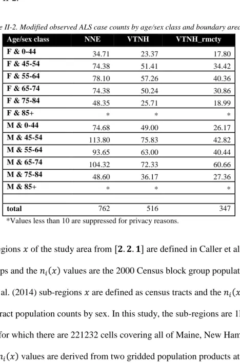
The modified case counts by age/sex and boundary area used to estimate age/sex specific rates are given in Table II-2.
Table II-2. Modified observed ALS case counts by age/sex class and boundary area
Age/sex class NNE VTNH VTNH_rmcty
F & 0-44 34.71 23.37 17.80 F & 45-54 74.38 51.41 34.42 F & 55-64 78.10 57.26 40.36 F & 65-74 74.38 50.24 30.86 F & 75-84 48.35 25.71 18.99 F & 85+ * * * M & 0-44 74.68 49.00 26.17 M & 45-54 113.80 75.83 42.82 M & 55-64 93.65 63.00 40.44 M & 65-74 104.32 72.33 60.66 M & 75-84 48.60 36.17 27.36 M & 85+ * * * total 762 516 347
*Values less than 10 are suppressed for privacy reasons.
The sub-regions 𝑥 of the study area from [𝟐. 𝟐. 𝟏] are defined in Caller et al. (2013) as census block groups and the 𝑛𝑖(𝑥) values are the 2000 Census block group population counts by sex. In Torbick et al. (2014) sub-regions 𝑥 are defined as census tracts and the 𝑛𝑖(𝑥) values are the 2000 Census tract population counts by sex. In this study, the sub-regions are 1km by 1km square grid cells, for which there are 221232 cells covering all of Maine, New Hampshire and Vermont and the 𝑛𝑖(𝑥) values are derived from two gridded population products at a 1km resolution representing the region’s population by the 12-age/sex classes at the year 2000. One
of the gridded population products is provided by the Socioeconomic Data and Applications Center (SEDAC) (Seirup & Yetman, 2006) and the other is a product of OakRidge National Laboratory (ORNL) called LandScan (LandScan 2000).
SEDAC’s 1km population product is lightly modeled meaning Census 2000 block counts were disaggregated using one data layer, while ORNL’s LandScan product uses more data layers. ORNL’s LandScan 2000 population product is also based off of population values of the 1990 Census projected to the year 2000. Given the difference in input variables used to model the populations between the two organizations, there is also a slightly different meaning to the population locations for each. SEDAC’s population estimates were modeled using nighttime lights and so represent nighttime population locations while LandScan represents daytime
populations (What Are the Differences Between GPW, GRUMP and Landscan? 2015). Neither of the SEDAC or LandScan 2000 1km population products are available by the age/sex classes defined in Noonan et al. (2005). Thus a simple approach that assumes demographic
characteristics are constant at the census block level was used to apply the age/sex class totals from the 2000 Census at the census block level. Although this assumption may not be true for large census blocks, this represents the best-known available data.
First, age/sex class proportions were calculated for each 2000 Census block within the NNE region. Then the shape file of Census 2000 block polygons was rasterized to a 20-meter resolution lattice with the same extent and origin as the 1km SEDAC lattice and all lattice cells with centroid in the same polygon received the age/sex count from that polygon. The 20-meter resolution was chosen since this was the smallest width or length dimension of any of the census block polygons. Rasterized census block age/sex proportions made up a 12-layer raster brick, where each layer contained the proportion of each census block population belonging to a
specific age/sex class. This 20-meter resolution raster brick was then aggregated to a 1km resolution by averaging the proportions in each layer separately. For a 1km cell falling
completely inside a census block, the 1km cell would have the same value as all the 20-m cells. For 1km cells intersecting several census blocks, the proportion represents an area-weighted average of proportions from different census blocks, and finally if regions with no population were included in the 1km cells, these regions were excluded in the average calculation. After age/sex proportions were aggregated to the 1km resolution, the 12 layers were summed in order to verify each cell had a value of either 1 (at least one of the age/sex classes is present) or 0 (no population). Each of the age/sex class proportion layers was then multiplied by the population counts for each SEDAC and LandScan 2000 separately. The LandScan 2000 global lattice at 1km resolution cropped to the NNE region had a slightly different origin than SEDAC’s NNE 1km population raster. Thus, population counts from the LandScan 2000 were resampled to match the SEDAC lattice.
Table II-3. Comparison of total population counts by age/sex class for all of NNE
Age/sex class Census blocks SEDAC LandScan
1 F & 0-44 971469 826144.9408 837851.9386 2 F & 45-54 236326 252879.8987 258295.7725 3 F & 55-64 146905 177108.8892 178379.3266 4 F & 65-74 115673 135658.4292 139148.6193 5 F & 75-84 85539 93696.24544 97578.34566 6 F & 85+ 37291 32589.75896 33682.87883 7 M & 0-44 979005 845637.6616 853779.2156 8 M & 45-54 234088 252396.0614 259875.2447 9 M & 55-64 142861 170199.82 173161.5455 10 M & 65-74 99533 124757.9363 126240.4717 11 M & 75-84 56594 67465.08834 68286.85924 12 M & 85+ 14252 14499.35824 14502.82532 13 Total Female 1593203 1518078.162 1544936.881 14 Total Male 1526333 1474955.926 1495846.162 15 Total (after) --- 2993034.088 3040783.044 16 Total (before) 3119536 3119535.991 3145258
Total population counts by age/sex class for the entire NNE region are summarized in the Table II-3. Rows 15 and 16 compare the total population estimate by SEDAC and LandScan 2000 before proportions were applied and afterward. Before proportion were applied the SEDAC total population for NNE matches the Census 2000 count, while the LandScan 2000 count is slightly larger. Recall, LandScan 2000 counts were developed before the 2000 US census was complete and is thus based on projections from the 1990 US census. After the proportions were applied, both the total populations for SEDAC and LandScan 2000 decrease. This is likely due to spatial uncertainty in locations without populations. Age/sex class differences between the Census blocks totals and calculated values for SEDAC and LandScan 2000 show that calculated values are less than Census values for both sexes younger than 45 and greater than Census values for both sexes older than 44 with the exception of females older than 84. It is important to note that all these estimates, Census 2000, SEDAC and LandScan 2000 contain some unquantifiable
uncertainty about the true population in this region for this time. However, by using two different estimates of expected counts, the effect of estimates can be partially quantified.
III DESCRIPTION OF ALS CASE AND EXPOSURE DATA
3.1NNEALSCASE DATA
The ALS case datasets discussed in Caller et al. (2013) and Torbick et al. (2014), included case data collected from medical records at Dartmouth Hitchcock Medical Center (DHMC) and the Muscular Dystrophy Association (MDA) of Northern New England. Both studies report a thorough data collection quality control process that only included cases having year of diagnosed (or in some cases year of MDA registration) between January 1997 and October 2009 and who had a primary address in Northern New England (NNE). The collected information about each case included age at diagnosis, side of symptom onset, year of diagnosis, year of death, family history, dwelling address at time of diagnosis, and in some instances historical dwelling addresses (Caller et al., 2013; Torbick et al., 2014). Note that given the uncertainty with some of the times of diagnosis, this data is more likely a representation of ALS prevalence, however since life expectancy for ALS patients is short, the prevalence will be close to the incidence.
In the current analysis, only the variables date of birth, sex, and longitude/latitude coordinates for an approximate dwelling address at time of diagnosis were made available from the ALS case dataset used in Caller et al. (2013) and Torbick et al. (2014) for reasons of
confidentiality. The dataset originally included 772 cases and also included two other columns, one with notes indicating additional information about the longitude/latitude coordinates and the
other with a color-coding of red, yellow, or none. Location information was missing (missing coordinates and location notes) for 8 of the 772 cases. Thus these 8 cases were excluded, and a total of 764 cases were used in the analyses that follow.
There are some additional uncertainties present in the 764 cases used in the following analyses that could have biased some results. In particular, location notes were only recorded for 22 of the remaining 764 cases of which 9 gave a town name and the other 11 indicated an error message. Since the cases with a town name note were missing longitude and latitude coordinates needed for summarizing the data on the computational grid, these cases were assigned a set of coordinates using the geocode function in the R package ggmap, which makes use of Google Maps (Kahle & Wickham, 2013). Unique town names were available for 7 of the 9 cases and these were assigned to town centroids, while the other 2 were assigned to a town hall location and a public library location within the town respectively. This procedure does add spatial uncertainty for distances less than the town aggregation level. Furthermore, 4 of the 764 cases, only contained 2 unique date of birth, sex and location combinations. Since, these are likely duplicate cases, in the analysis of ALS within the VTNH boundary, 2 of these 4 cases were removed, giving a total of 762 cases considered. Despite the uncertainties in the ALS case data used for the following analyses, the author believes the data are sufficient for the goals outlined at the beginning of this dissertation.
3.2EXPOSURE METRICS FOR WATER QUALITY
There are several hypothesized routes by which people may be exposed to BMAA, the neurotoxin produced by cyanobacteria (blue-green algae) that is suspected to be a risk factor for ALS. These include drinking water, water sport activities such as swimming and boating, aerosolization of cyanobacteria blooms, and dietary exposure from eating seafood (Caller et al.,
2013). In Northern New England, there are over 6,000 water bodies that could pose as a possible exposure source. Given the costs, both in time and money, of traditional water quality
assessment needed for these over 6,000 water bodies, the use of satellite remote sensing
technology is a viable alternative. The choice of a particular satellite sensor depends on the goals of the application since the spatial and temporal resolutions as well as the spectral sensitivity vary between different technologies. This application requires a fine spatial resolution with
sufficient spectral sensitivity to derive metrics related to cyanobacteria for the entire NNE region. Torbick et al. (2014) show that the Landsat Thematic Mapper is a useful tool for deriving
cyanobacteria related water quality metrics at 30 meter resolution pixels covering all lakes sized 6 hectares or more in NNE, through the use of band ratio regression techniques calibrated with in-situ lake sampled measurements.
3.2.1 Torbick et al. (2014) Water Quality Metrics
The water quality metrics used by Torbick et al. (2014) to explain census tract based ALS cluster membership include secchi depth (SD in meters), total nitrogen (TN in micrograms per liter (ug/L)), and chlorophyll-a (Chl-a in ug/L), and were derived from Landsat images taken in late August and early September (days of year 242, 244, 248) for the years 2009 and 2010. Lake averages of these metrics were calculated for all lakes sized 6 hectares or more, which included a total of 4453 lakes for which 3298 were found in Maine, 925 in New Hampshire, and 230 in Vermont. The average for Lake Champlain however was not included since it is located at the very western boundary of NNE and is likely not well represented by one average value due to its size (Torbick et al., 2014).
Figure III-1. Distribution of lake average SD, TN and Chl-a satellite derived metrics for all 4453 lakes in NNE greater than 6 hectares. Top: Metric boxplots of all lakes; Bottom: Metric histogram of non-outliers values only.
The box plots in Figure III-1 show that some of the satellite derived SD, TN and Chl-a metrics have values outside the range of observed in-situ measurement values of these metrics (values beyond red line). In particular, values of SD greater than 69 meters, TN greater than 30 ug/L and Chl-a greater than 200 ug/L were marked as outliers as these values are highly
improbable for lakes in NNE. In general, both TN and Chl-a values have a positive skew (bottom of Figure III-1), and in general are positively correlated (Figure III-2): lakes with low average Chl-a values also have low average TN values.
Figure III-2. Late Summer 2009/2010 snapshot values of lake average secchi depth, total nitrogen, and chlorophyll-a for lchlorophyll-akes sized 6 hectchlorophyll-ares for more chlorophyll-across Northern New Englchlorophyll-and
Torbick et al. (2014) reports that these metrics show most water bodies in NNE over 6 hectares are considered healthy waters for this late summer 2009/2010 time snapshot, while only about 4% would be considered nutrient-rich lakes in which frequent and intense algal blooms would be likely to occur. Maps in Figure III-2 show a spatial distribution of these water quality metrics with the warmer colors (red/orange) indicating poorer water quality. In particular, in the right most map, lakes colored orange have Chl-a values that the World Health Organization (WHO) would classify as a moderate acute health risk and lakes colored red have Chl-a values that classify as a high acute health risk according to their guidelines for recreational waters (Guidelines and Recommendations 2016).
3.2.2 Phycocyanin (PC) Metric
Another satellite-derived metric used in this study that is related to the presence of cyanobacteria is phycocyanin (PC in ug/L). Phycocyanin is generally positively correlated with Chl-a and TN and negatively correlated with SD. This metric however is thought to be more closely related than Chl-a, TN and SD to the amount of BMAA to which the population is
exposed since phycocyanin is a pigment of the cyanobacteria that produce the BMAA. Although, there is evidence for a disparity between the presence of cyanobacteria and the toxins it produces, which is not well understood as there is little mechanistic understanding related to why and when cyanobacteria produce toxins (Loftin et al., 2016).
The PC metric used in this study represents a late summer 2014/2015 snapshot of the amount of PC (ug/L) in all 30 meter water pixel covering all lakes sized 6 hectares or more (Figure III-3).
Figure III-3. Late Summer 2014/2015 Snapshot Representation of the amount of phycocyanin for each 30m water pixel for all lakes sized 6 hectares or more in Northern New England
Lake averages of these pixel PC values range from about 0 to 1200 ug/L with the majority of lake averages below 10 ug/L (Figure III-4).
Figure III-4. Lake average phycocyanin (ug/L) for 4867 lakes sized 6 hectares or more across Northern New England based on Landsat derived metric at 30 meter resolution pixels.
3.2.3 Tropic Status Index (TSI) Metric
Trophic Status Index (TSI) is an ordinal metric used by ecologists to classify water bodies based on their varying amounts of nutrients and is an indicator of water health (Carlson 1977). Generally, an entire water body is given one classification, however for large water bodies with spatially varying amounts of nutrients, sections of the water body may be classified differently. Index values are 1: oligotrophic, 2: mesotrophic: 3: eutrophic and 4: hypereutrophic, where eutrophic and hypereutrophic water bodies contain the most nutrients. These lakes are most likely to experience frequent and intense algae blooms, while oligotrophic lakes are clear and good sources of drinking water. A number of metrics may be used to classify the trophic status of a water body including amounts of total nitrogen, total phosphorus, abundance of algae, total chlorophyll-a, and secchi depth.
This study considers a TSI metric based on secchi depth derived from the spectral bands of Landsat Thematic Mapper calibrated using in-situ secchi depth measurements from lakes across the Continental United States that were included in the National Lake Assessment 2007. This TSI metric gives a classification for each 30-meter water pixel covering all lakes in
Northern New England sized 6 hectares or more for the particular day and year of a Landsat overpass. A lake classification for a particular day and year is based on the mode (most common) classification of all 30-meter water pixels within a given lake. Due to its size, a lake
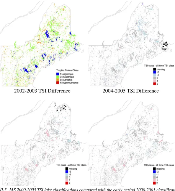
classification was not given to Lake Champlain. Lake classifications based on Landsat images taken during the months of July, August and September (JAS) for the years between 2000 and 2005, were then used to calculate JAS classifications for the time periods, 2000 to 2001, 2002 to 2003, 2004 to 2005 and 2000 to 2005. JAS classifications were determined by using the median classification of all 50% cloud free Landsat overpass dates within the specified time period for each lake. The JAS 2000-2005 TSI lake classifications for lakes (n=5,809) across NNE are shown in Figure III-5. The three other time period lake classifications are compared to the JAS 2000-2005, where blue colors indicate a clearer classification than the one for 2000-2005 and red colors indicate a murkier classification than the one for 2000-2005.
JAS 2000-2005 Lake TSI 2000-2001 TSI Difference
2002-2003 TSI Difference 2004-2005 TSI Difference
Figure III-5. JAS 2000-2005 TSI lake classifications compared with the early period 2000-2001 classification, the middle period 2002-2003 classification and the late period 2004-2005 classification.
Landsat overpass dates vary by location in NNE because Landsat has a square footprint of about 180km and requires 12 frames to create wall-to-wall maps of TSI across all NNE. Furthermore, approximately 10 to 11 Landsat overpass dates are possible in a given year. However, the number of images available for each lake will vary by location because adjacent Landsat orbit paths overlap resulting in additional observations of some lakes and cloud cover also varying by day and location will result in less observations for other lakes. Overpass
frequency and day of year variability by location for each of these time periods is shown in Figure III-6 and Figure III-7 respectively.
2000-2005 (all years) 2000-2001 (early)
2002-2003 (middle) 2004-2005 (late)
Figure III-6. Number of 50% cloud free Landsat overpasses by lake for each time period
The variability in cloud-free overpass dates and frequency may explain some of the variability in TSI values between time periods, but more research is need to fully characterized the effects of the irregular sampling pattern on the TSI spatial variability across NNE. However, almost half the lakes (n=2813) have the same classification for all time periods and only about 6% of lakes (n=330) vary by 2 or 3 classes.
2000-2005 (all years) 2000-2001 (early)
2002-2003 (middle) 2004-2005 (late)
Figure III-7. Average time of month for all 50% cloud free Landsat overpass dates by lake for each time period.
3.2.4 Lake Champlain Surface Water Temperatures
Lake water temperature is a central driver regulating lake ecology. Recent studies suggest temperatures are increasing in many inland lakes (Schneider & Hook, 2010; Smeltzer,
Shambaugh, & Stangel, 2012; Torbick, Ziniti, Wu, & Linder, 2016). These temperature increases are suspected to increase the frequency, magnitude, and duration of cyanobacterial harmful algal blooms. Understanding the spatio-temporal dynamics of lake temperature change may provide
valuable insight in how other ecological processes vary within the lake, including the development and duration of algal blooms.
Lake Champlain is the largest lake in the NNE region for which there exists several valuable long-term water temperature records and thus is an ideal candidate for a case study of the spatio-temporal dynamics of lake temperature change. In a previous study, temperature data from two water monitoring programs, a survey by early limnologists E.B Henson and M. Potash from the University of Vermont from 1964 to 1974 and the Long-Term Water Quality and Biological Monitoring Program on Lake Champlain supported by the Lake Champlain Basin Program from 1992 to 2009, were analyzed showing that August mean surface water
temperatures of Lake Champlain rose by 1.6-3.8 degrees Celsius between 1964 and 2009 (Smeltzer et al., 2012). Furthermore, this increase was statistically significant for 8 out of the 10 sampling sites considered. It is likely that the temperature trends at nearby sites exhibit positive spatial autocorrelation and that trends could be calculated with less uncertainty, if this
autocorrelation is included in the calculation. The limited number of sites in this previous study however do not provide sufficient information to make this modeling useful. On the other hand, Landsat Thermal Imagery can be used instead since the spectral bands provide satellite-derived measurements of water temperature for a 31-year period from 1984 to 2014 in a 30 by 30 meter uniform gridded format covering the entire lake.
For this case study, surface water temperatures derived from Landsat images calibrated to in-situ water measurements were collected for the months of July, August, and September (JAS) for the investigation of the summertime spatio-temporal temperature trends within Lake
Champlain. Only Landsat images of path row tile 014029, which covers most of Lake Champlain except for the very narrow southern section were included and the JAS metric was chosen to
represent temperatures in which algae most commonly bloom. Two Landsat satellites were in operation during the 31-year period, each having a 16-day interval between images. Landsat LT5 captured images during the years 1984 to 2012 and Landsat LE7 began collecting in 1999 with an 8-day collection offset to Landsat LT5 (Figure III-8).
Figure III-8. Sampling Pattern of Landsat LT5 and LE7 for mostly cloud free images of path row tile 014029 over Lake Champlain
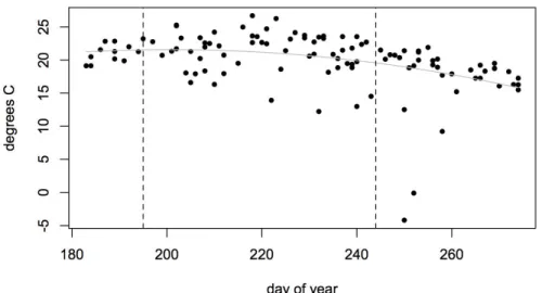
Although the two satellites cumulatively captured a total of 270 images of tile 014029 during this period, only 114 of these images could be used to calculate water temperatures due to poor image quality and/or extensive cloud cover. Also day of year sampling patterns vary from year to year. In particular no samples before day of year 200 are available for years before 1999, and the sampling frequency is very sparse or nonexistent for years after 2011. Furthermore, average lake temperatures exhibit a systematic quadratic variability by day of year for the July to September collection months (Figure III-9).
Figure III-9. Average lake satellite-derived surface water temperatures of Lake Champlain from 1984-2014 by day of year
Thus, to control for trend bias due to the sparse and irregular sampling pattern and due to the day of year variability, only images taken between day of year 195 and 244 and for years before 2012 were used for spatio-temporal trend estimates. This gave a total of 63 time points over the 27-year period from 1984 to 2011.
Satellite derived temperatures also have the potential for more noise than in-situ
measured temperatures due to varying atmospheric conditions. Figure III-10 shows that there are a number of outlier values, particularly lower outliers, in the satellite-derived temperatures of Lake Champlain compared with in-situ buoy measured temperatures.
Figure III-10. Satellite-derived surface water temperatures of Lake Champlain from 1984-2011 for days of year 195 to 244 vs. buoy in-situ water temperatures from 1992-2013 for days of year 195 to 244 and depths below 4 meters. (Gray line at 16 degrees Celsius.)