low-resolution density map using three-dimensional
orthogonal Hermite functions
Georgy Derevyanko, Sergei Grudinin
To cite this version:
Georgy Derevyanko, Sergei Grudinin. HermiteFit: fast-fitting atomic structures into a
low-resolution density map using three-dimensional orthogonal Hermite functions. Acta
Crystallo-graphica Section D: Biological Crystallography, International Union of Crystallography, 2014,
70 (8), pp.2069-2084.
<
10.1107/S1399004714011493
>
.
<
hal-01078550
>
HAL Id: hal-01078550
https://hal.inria.fr/hal-01078550
Submitted on 1 Feb 2016
HAL
is a multi-disciplinary open access
archive for the deposit and dissemination of
sci-entific research documents, whether they are
pub-lished or not.
The documents may come from
teaching and research institutions in France or
abroad, or from public or private research centers.
L’archive ouverte pluridisciplinaire
HAL, est
destin´
ee au d´
epˆ
ot et `
a la diffusion de documents
scientifiques de niveau recherche, publi´
es ou non,
´
emanant des ´
etablissements d’enseignement et de
recherche fran¸
cais ou ´
etrangers, des laboratoires
publics ou priv´
es.
Acta Crystallographica Section D
Biological Crystallography
ISSN 1399-0047
HermiteFit
: fast-fitting atomic structures into a
low-resolution density map using three-dimensional
orthogonal Hermite functions
Georgy Derevyanko and Sergei Grudinin
Acta Cryst.
(2014). D70, 2069–2084
Copyright c⃝International Union of Crystallography
Author(s) of this paper may load this reprint on their own web site or institutional repository provided that this cover page is retained. Republication of this article or its storage in electronic databases other than as specified above is not permitted without prior permission in writing from the IUCr.
For further information seehttp://journals.iucr.org/services/authorrights.html
Acta Crystallographica Section D: Biological Crystallography welcomes the submission of papers covering any aspect of structural biology, with a particular emphasis on the struc-tures of biological macromolecules and the methods used to determine them. Reports on new protein structures are particularly encouraged, as are structure–function papers that could include crystallographic binding studies, or structural analysis of mutants or other modified forms of a known protein structure. The key criterion is that such papers should present new insights into biology, chemistry or structure. Papers on crystallo-graphic methods should be oriented towards biological crystallography, and may include new approaches to any aspect of structure determination or analysis. Papers on the crys-tallization of biological molecules will be accepted providing that these focus on new methods or other features that are of general importance or applicability.
Acta Crystallographica Section D
Biological Crystallography
ISSN 1399-0047
HermiteFit
: fast-fitting atomic structures into a
low-resolution density map using three-dimensional
orthogonal Hermite functions
Georgy Derevyankoa,b,c,d,eand
Sergei Grudininf,g,h*
aInstitute of Complex Systems (ICS-6), Forschungszentrum Ju¨lich, Ju¨lich, Germany, bUniversite´ Grenoble Alpes, IBS,
F-38000 Grenoble, France,cCNRS, IBS, F-38000 Grenoble, France,dCEA, IBS, F-38000 Grenoble, France,e Research-Educational Centre Bionanophysics, Moscow Institute of Physics and Technology, Dolgoprudniy, Russia,fUniversite´ Grenoble Alpes, LJK, F-38000 Grenoble, France,gCNRS, LJK, F-38000 Grenoble, France, andhINRIA, France
Correspondence e-mail: sergei.grudinin@inria.fr
#2014 International Union of Crystallography
HermiteFit, a novel algorithm for fitting a protein structure into a low-resolution electron-density map, is presented. The algorithm accelerates the rotation of the Fourier image of the electron density by using three-dimensional orthogonal Hermite functions. As part of the new method, an algorithm for the rotation of the density in the Hermite basis and an algorithm for the conversion of the expansion coefficients into the Fourier basis are presented.HermiteFitwas implemented using the correlation or the Laplacian-filtered cross-correlation as the fitting criterion. It is demonstrated that in the Hermite basis the Laplacian filter has a particularly simple form. To assess the quality of density encoding in the Hermite basis, an analytical way of computing the crystallographic R
factor is presented. Finally, the algorithm is validated using two examples and its efficiency is compared with two widely used fitting methods, ADP_EM and colores from the Situs
package. HermiteFit will be made available at http:// nano-d.inrialpes.fr/software/HermiteFit or upon request from the authors.
Received 21 January 2013 Accepted 19 May 2014
1. Introduction
An important class of algorithms in computer science deals with the exhaustive search in six-dimensional space of trans-lations and rotations of a rigid body. These algorithms are used, for example, in crystallography for molecular replace-ment and in computational biology to perform ligand docking, to predict protein–protein interactions and to discover the structures of macromolecular assemblies.
Modern exhaustive search algorithms implement either a fast three-dimensional translational search using the fast Fourier transform (FFT; Chaco´n & Wriggers, 2002; Katchalski-Katziret al., 1992; Gabbet al., 1997; Wriggers, 2010; Siebert & Navaza, 2009) or a fast three-dimensional rotational search by means of spherical harmonics decomposition and the FFT (Kovacs & Wriggers, 2002; Crowther, 1972), or even a fast five-dimensional rotational search (Kovacs et al., 2003; Ritchie
et al., 2008). An exhaustive search is also widely used as a preliminary step preceding local search or flexible refinement procedures. Thus, the quality and the speed of exhaustive search algorithms have a great impact on the solution of a vast variety of problems. Therefore, we believe that new directions of research on this topic are very important and highly valu-able.
In this paper, we present the new HermiteFit algorithm that uses orthogonal Hermite functions to perform an exhaustive search in the six-dimensional space of rigid-body motions. We apply this method to the problem of fitting of a
high-resolution X-ray structure of a protein subunit into the cryo-electron microscopy (cryo-EM) density map of a protein complex. As part of this new method, we developed an algo-rithm for the rotation of the decomposition in the Hermite basis and another algorithm for the conversion of the Hermite expansion coefficients into the Fourier basis.
The choice of the application of our algorithm is dictated by the fact that currently the major source of information on the mechanisms of function of proteins and their assemblies are the atomic structures obtained by X-ray crystallography. However, as the size of the protein grows, as often happens in protein complexes, it becomes more difficult to obtain well ordered crystals that are sufficiently large for X-ray experi-ments. Hopefully, in many cases, different parts of the protein complex can be crystallized separately. Usually, their struc-tures can be solved to atomic resolution. The whole protein complex in this case can be probed by cryo-EM (Cheng & Walz, 2009), by small-angle X-ray scattering (Svergun & Koch, 2003) and with recent advances in femtosecond X-ray lasers (Chapmanet al., 2011). Usually, these techniques provide of an electron-density map (EDM) of a large protein or a protein complex with a resolution lower than 3.5 A˚ , whereas the atomic structures of its small subunits can be solved with X-ray crystallography at even sub-angstrom resolution. To recon-struct large proteins or protein complexes at high resolution, the high-resolution crystallographic structures of small units can be fitted into the low-resolution structures of the whole assembly. A number of software packages have been devel-oped for this task. The most notable of them are Situs
(Wriggers, 2010; Chaco´n & Wriggers, 2002),NORMA(Suhre
et al., 2006), EMFit (Rossmann et al., 2001) and UROX
(Siebert & Navaza, 2009). Despite the differences in their implementation, all of the algorithms maximize some score that shows the goodness of the fitting using a certain optimi-zation algorithm. An excellent review of the different types of scoring functions used for cryo-EM density fitting is given by Vasishtan & Topf (2011). According to them, one of the most popular scoring functions is the cross-correlation function (CCF) between the EDM and the density of the fitted protein. Given a protein structure that is described by its electron densityf(r), and an EDM obtained from, for example, a cryo-EM experiment described by the functiong(r), we can mini-mize the square-root discrepancy between them. Precisely, this discrepancy is given by
S¼R½TT^RRf^ ðrÞ %gðrÞ&2dr; ð1Þ where TT^ andRR^ are the operators of the translation and the rotation, respectively, applied to the density f(r). We can rewrite the scoring functionSas
S¼R½TT^RRf^ ðrÞ&2drþRg2
ðrÞdr%2RTT^RfR^ ðrÞgðrÞdr: ð2Þ Therefore, minimization of the scoreSis equivalent to maxi-mization of the CCF,
CCF¼RTT^RRf^ ðrÞgðrÞdr; ð3Þ
with respect to the parameters of the operatorsTT^ andRR^. This scoring function has been used in the majority of the algo-rithms and software packages that perform fitting to the EDM (Wriggers, 2010; Siebert & Navaza, 2009; Suhreet al., 2006).
Another widely used scoring function is the Laplacian-filtered cross-correlation function (LCCF). It originated from the observation that a human performing a manual fitting of a structure into an EDM tends to match the isosurfaces of the densities rather than the densities themselves,
LCCF¼R½!TT^RRf^ ðrÞ&½!gðrÞ&dr: ð4Þ This scoring function works better than the CCF for low-resolution maps ((10–30 A˚ ; Wriggers, 2010) and was used for the first time in the CoAn/CoFialgorithm (Volkmann & Hanein, 1999). Other scoring functions that, for example, penalize symmetry-induced protein–protein contacts, or make use of protein–protein docking potentialsetc., have also been developed (Vasishtan & Topf, 2011). In our work, we use the CCF and LCCF to determine the goodness of fit.
In this paper, we demonstrate the ability of our algorithm to compete with the well established approaches by using two examples of different difficulty: the PniB conotoxin peptide and the GroEL complex. The first example illustrates the encoding principles and demonstrates the influence of the encoding quality on the goodness of fit. The second example is the gold standard of all electron-density map-fitting algo-rithms. Our approach allows analytical assessment of the quality of encoding of the Hermite basis using an estimation of the crystallographicRfactor. We then compare this estimation with that computed numerically for the PniB conotoxin density map. Finally, we compare the speed and the fitting accuracy of our algorithm with two popular programs, the
ADP_EM fitting method and the coloresprogram from the
Situs package, and demonstrate that HermiteFit takes less running time per search point compared with the two other methods while attaining a similar accuracy.
TheHermitFitalgorithm can be straightforwardly applied to a broad class of problems in different fields of research. For example, one of the bottlenecks of algorithms for molecular replacement in crystallography is the computation of the Fourier coefficients (structure factors) of a molecule (Navaza & Vernoslova, 1995). This operation needs to be precise and fast. However, exact analytical evaluation of the structure factors is too costly (Sayre, 1951) when recomputing them for each rotation of the molecule. Therefore, currently one uses the Sayre–Ten Eyck approach to compute the Fourier coeffi-cients (Ten Eyck, 1977). Unfortunately, one has to be very careful tuning the parameters of the electron-density model and the grid cell size to obtain the desired precision (Navaza, 2002; Afonine & Urzhumtsev, 2004). Unlike the Sayre–Ten Eyck approach, our algorithm offers an analytical expression for the structure factors of the Hermite decomposition of a molecule. Finally, our approach allows analytical estimatation of the quality of encoding using, for example, crystallographic
2. Methods
2.1. Summary of the standard fitting algorithm
The standard FFT-based three-dimensional fitting algo-rithm operates according to the workflow shown in Fig. 1 (Katchalski-Katzir et al., 1992; Gabb et al., 1997; Chaco´n & Wriggers, 2002). The input of this algorithm is a protein atomic structure determined experimentally by, for example, X-ray crystallography or nuclear magnetic resonance (NMR) experiments. Another input is an experimental EDM deter-mined by means of, for example, cryo-EM. Firstly, the algo-rithm decomposes the experimental EDM into the Fourier basis using the fast Fourier transform algorithm. It then rotates the protein structure to a certain orientation r and decomposes the electron density of the rotated structure into the Fourier basis. The electron density is typically computed as a sum of Gaussians centred on non-H atoms of the protein. Afterwards, the algorithm exhaustively explores translational degrees of freedom of the rotated protein with respect to the EDM. For every translationt, it determines the corresponding score, which is usually given by the correlation between the two densities. This procedure is equivalent to computing the convolution of two functions,
CCFðr;tÞ ¼Rfðr;x%tÞgðxÞdx; ð5Þ wheref(r,x%t) is the density of the protein rotated byrand translated bytandg(x) is the experimental electron-density map. To speed up this step, the algorithm computes the values of the Fourier transform of the CCF for all translational degrees of freedom at once using the convolution theorem. Finally, the algorithm computes the inverse Fourier transform (IFT) of the convolution, generates a new rotation of the
protein structure and returns to the second step. This proce-dure is repeated until all rotational degrees of freedom of the protein with respect to the EDM have been explored (see Fig. 1). The solution of the fitting problem is then given by (rmax,tmax) = argmaxr,t[CCF(r,t)].
The bottleneck of the standard algorithm is the re-projec-tion of the protein electron density into the Fourier space after each rotation. To overcome this, we propose encoding the electron density of the protein structure in the orthogonal Hermite basis prior to performing the rotational search. This allows the projection of the protein density into the Fourier space to be sped up. Since only members of the Fourier family of linear transforms can replace the O(N2) operations of a
convolution in a time domain by O(N) operations in a frequency domain (Stone, 1998), we still need to perform the convolution in the Fourier space. Fig. 2 shows the workflow of the proposed algorithm. The computational complexity of this algorithm is listed in Table 1.
Table 1
Complexity of the Hermite fitting algorithm.
Here,Mdenotes the order of the Fourier decomposition,Nis the order of the Hermite decomposition,Natomis the number of atoms in the protein andNrot
is the number of rotations to be sampled.
Operation Complexity
Loop multiplier
Decomposition of the step function O(M3logM3) 1
Decomposition of the Gaussian O(NatomsN3) 1
Construction of the rotation matrix O(NrotN4) 1
Rotation O(N4) Nrot
Evaluation of the Hermite series O(M3N+M2N2+MN3) N rot
Multiplication O(M3) N
rot
Inverse Fourier transform O(M3logM3) N
rot
Figure 2
Flowchart ofHermiteFit, the new fitting algorithm based on Hermite expansions. Green blocks correspond to operations in Fourier space. Blue blocks correspond to operations in Hermite space.
Figure 1
2.2. Hermite functions
The orthogonal Hermite function of ordernis defined as
nðx;!Þ ¼ !1=2 ð2nn!"1=2Þ1=2exp % !2x2 2 ! " Hnð!xÞ; ð6Þ
where Hn(x) is the Hermite polynomial and !is the scaling
parameter. In Fig. 3 we show several orthogonal Hermite functions of different orders with different parameters !. These functions form an orthonormal basis set in L2
ðRÞ. A one-dimensional function f(x) decomposed into the set of one-dimensional Hermite functions up to orderNis given by
fðxÞ ¼P
N
i¼0
^
ffi iðx;!Þ: ð7Þ
Here, ff^i are the decomposition coefficients, which can be
determined from the orthogonality of the basis functions i(x; !). Decomposition of (7) is called band-limited decomposition with i(x;!) basis functions. To decompose the EDM and the protein structures, we employ the three-dimensional Hermite functions
n;l;mðx;y;z;!Þ ¼ nðx;!Þ lðy;!Þ mðz;!Þ; ð8Þ
which form an orthonormal basis set in L2 ðR3
Þ. A function
f(x,y,z) represented as a band-limited expansion in this basis is given by fðx;y;zÞ ¼P N i¼0 P N%i j¼0 P N%i%j k¼0 ^ ffi;j;k i;j;kðx;y;z;!Þ: ð9Þ
2.3. Decomposition of electron densities into the orthogonal Hermite basis
One of the advantages of the orthogonal Hermite basis is that we can derive the exact analytical expression for the decomposition coefficients of a molecular structure. This allows the exact decompositions to rapidly be obtained
without costly numerical integration over three-dimensional space. In our algorithm, the electron density of the protein [f(x) in equation 5, upon which rotation and translation operators act] is expanded in the Hermite basis using the Gaussian model. More precisely, we model the electron density of a single atom in the molecular structure as a Gaussian centred at the atomic positionrð0iÞ with the squared
variance equal to #2/2. The electron density of the whole
molecular structure is then given by the following sum,
MðrÞ ¼ P Natoms i¼1 exp½%jr%rð0iÞj 2=#2 &; ð10Þ whererð0iÞ is the position of theith atom,#/21/2is the variance
of the Gaussian distribution and r¼ ðx;y;zÞ2R3 is the sampling volume. Normally, each Gaussian should be weighted with a coefficient corresponding to the electron distribution of a particular atom. However, we omit the weights in our approximation. In Appendix A, we provide analytical expressions (equations 48 and 54) for the decom-position coefficients of M(r) in the one-dimensional and the three-dimensional cases.
2.4. Laplacian filter in the Hermite basis
For medium- to low-resolution maps the Laplacian-filtered cross-correlation function gives a better match compared with the CCF (Wriggers, 2010). In the Hermite basis, the Laplacian filter has a particularly simple form. Using the well known recurrence relation for the derivatives of Hermite functions, we can easily derive the following relation for the second derivative of a one-dimensional basis function:
d2 dx2 nðx;!Þ ¼ !2 2f½nðn%1Þ& 1=2 n%2ðx;!Þ þ ð2nþ1Þ nðx;!Þ þ ½ðnþ1Þðnþ2Þ&1=2 nþ2ðx;!Þg: ð11Þ
A similar relationship holds for the coefficients of the decomposition:
Figure 3
Left, one-dimensional Hermite functions of order six for three different scaling parameters!. Right, one-dimensional Hermite functions of two different orders for the scaling parameter!= 1.
^ h h00n¼ !2 2 f½nðn%1Þ& 1=2^ h hn%2þ ð2nþ1Þhh^n þ ½ðnþ2Þðnþ1Þ&1=2hh^nþ2g; ð12Þ
wherehh^nandhh^00nare thenth-order decomposition coefficients
of the original basis and its Laplacian representation, respectively. Forn < 0 andn> Nwe lethh^n = 0 andhh^00n = 0.
Owing to the properties of the Laplace operator and the three-dimensional Hermite decomposition, the contributions of the derivatives along each axis are additive. The derivation of the formula for the three-dimensional decomposition derivative is straightforward and we omit it for brevity.
2.5. Rotation of the Hermite decomposition
Recently, Parket al.(2009) presented a method to perform an in-plane rotation of a two-dimensional orthogonal Hermite band-limited decomposition. Here, we extend their method to the three-dimensional case. Let us first consider the decom-position of a two-dimensional function into a two-dimensional orthogonal Hermite-function basis,
fðx;yÞ ¼P N n¼0 P N%m m¼0 ^ ffn;m nðx;!Þ mðy;!Þ: ð13Þ
The decomposition of a functionf$(x,y) rotated clockwise by an angle$is given by f$ðx;yÞ ¼ P N m¼0 Pm k¼0 Pm n¼0 ^ ffn;m%nSmk;n ! " kðx;!Þ m%kðy;!Þ; ð14Þ
where the coefficientsSkm,nare computed using the following
recurrent formulae (Parket al., 2009):
Smq;þn1¼ n m%qþ1 ! "1=2 sinð$ÞSmq;n%1þ m%nþ1 m%qþ1 ! "1=2 cosð$ÞSmq;n; Smq;þ01¼ mþ1 m%qþ1 ! "1=2 cosð$ÞSmq;0; Smmþþ11;n¼ n mþ1 ! "1=2 cosð$ÞSmm;n%1% m%nþ1 mþ1 ! "1=2 sinð$ÞSmm;n; Smmþþ11;0¼ %sinð$ÞSmm;0: ð15Þ
The key idea that allows the generalization of these formulae to a three-dimensional decomposition is that we can factorize a rotation in three-dimensional space into three independent
in-plane rotations about three different axes and then rotate each two-dimensional decomposition using (14). Let us consider the following three-dimensional decomposition:
fðx;y;zÞ ¼P N n¼0 nð x;!ÞP N%n m¼0 P N%m%n l¼0 ^ ffn;m;l mðy;!Þ lðz;!Þ: ð16Þ
If we rotate this decomposition about thexaxis, this rotation will be equivalent toNrotations of different two-dimensional decompositions in theyzplane,
fnðy;zÞ ¼ P N%n m¼0 P N%m%n l¼0 ^ ffn;m;l mðy;!Þ lðz;!Þ: ð17Þ
This observation means that in order to perform such a rotation, we need to recompute a rank 3 tensor of coefficients
^
ffn;m;l slice by sliceN times using (14). Fig. 4 illustrates three
subsequent rotations of the tensorff^n;m;l. Each rotation of the
coefficients in one plane corresponds to a multiplication of these coefficients by a rotation matrix. Therefore, a three-dimensional rotation defined with three Euler angles is equivalent to three sequential rotations of coefficients in three planes.
2.6. Transition from the Hermite to the Fourier basis
In order to perform a fast convolution as in (5), we convert the decomposition coefficients from the Hermite basis into the Fourier basis. This allows use of the fast convolution algorithm based on the Fourier convolution theorem, which was first introduced in protein–protein docking studies (Katchalski-Katzir et al., 1992; Gabb et al., 1997) and then also applied to EDM fitting (Chaco´n & Wriggers, 2002; Wriggers, 2010; Siebert & Navaza, 2009). The key idea of this algorithm is to compute the Fourier transform of the values of a scoring function on a grid, CCF(r,t) =Rfðr;xÞgðr;x%tÞdx, using the convolution theorem
Fðf*gÞ ¼FðfÞFðgÞ; ð18Þ
i.e.by multiplying the complex-conjugated coefficients of the Fourier transform of the protein electron density with the coefficients of the Fourier transform of the EDM. We then obtain CCF(r, t) by taking the inverse Fourier transform of
Fðf*gÞ,
Figure 4
Sequential rotations of coefficients^ffn;m;labout different axes. The rotated layer is shown with solid cubes; other coefficients are shown with dashed cubes.
To perform the complete rotation of the decomposition about one axis, we rotate each layer of coefficients about the corresponding axis in the coefficient space.
CCFðr;tÞ ¼IFT½FðfÞFðgÞ&: ð19Þ Now we explain how we convert the decomposition coeffi-cients from the Hermite basis into the Fourier basis. Consider the decomposition of a functionf(r) in the three-dimensional Hermite basis with decomposition coefficients ff^i;j;k (9). The
orthogonal Hermite functions are the eigenfunctions of the continuous Fourier transform,
R nðx;!Þexpð%2"i!xÞdx¼ ð%iÞ n n !; 2" ! ! " + ~nð!;!Þ; ð20Þ where ! is the frequency in reciprocal space. In order to compute Fourier coefficients of f(r) to order M, we first compute the Fourier transforms of the basis functions i(x;!),
j(y; !) and k(z; !) using (20). We then substitute these coefficients into (9) and obtain the following expression for
~
ffl;m;n, the Fourier coefficients off(r):
~ ffl;m;n¼ 1 LxLyLz PN i¼0 P N%i j¼0 P N%i%j k¼0 ^ ffi;j;k i~ l Lx;! ! " ~ j m Ly;! ! ~ k n Lz;! ! " : ð21Þ
These values can be computed in O(M3N + M2N2 + M3N) steps (see AppendixB).
2.7. Implementation details and running time
We chose to demonstrate the potential of the Hermite basis by implementing the rigid-body fitting of an atomistic struc-ture of a protein in an electron-density map of low resolution. The HermiteFit algorithm was implemented using the C++ programming language and compiled using g++ with -O3 optimization. The running times of the tested algorithms were measured on a single core of an Intel Xeon CPU X5650 @2.67 GHz processor with 24 GB of RAM on a Linux 64-bit operating system.
Our fitting method typically samples some 1010rigid-body configurations. Therefore, it is practical to group its fitting solutions into clusters. There are multiple ways to measure the similarity between rigid-body solutions. For example, the pairwise root-mean-square deviation (r.m.s.d.) is a fast and well accepted similarity measure. Thus, we clustered the fitting solutions using the rigid-body clustering algorithm imple-mented with the RigidRMSD library (Popov & Grudinin, 2014) as follows. Firstly, the fitting solution with the best score (yet unassigned to any cluster) is taken as the seed for the new cluster. Secondly, the pairwise r.m.s.d.s between the seed and all other predictions are measured and predictions with an r.m.s.d. lower than a certain threshold are put into the cluster. Finally, these two steps are iterated until all fitting predictions are assigned to corresponding clusters.
3. Analysis
This section provides analytical and numerical analysis of the density encoding in the Hermite basis. More specifically, we provide the choice of optimal model parameters and assess the quality of encoding.
3.1. Choice of parameters of the method
Orthogonal Hermite functions (6) decay exponentially after a certain distance and thus can encode information only within some interval. We can estimate this interval using the formula for the last root of a Hermite polynomial,%1,N’(1 + 2N)1/2/!
(Ricci, 1995), which gives an approximation for the half-size of the bounding box that we can successfully encode:
Lbox=2<(ð
1þ2NÞ1=2
! : ð22Þ
On the other hand, orthogonal Hermite functions are the eigenfunctions of the continuous Fourier transform (20).
Figure 5
Absolute values of the two matricesF(1)andF(2)that give the transfer matrix as their product (35). These matrices are computed with scaling parameter
!= 0.55 and input box sizeLbox= 23.0 A˚ , which mimics the first fitting example shown below. Left,F(1), the scaled Fourier transform of a
one-dimensional Hermite function, as given by (36). Right,F(2), the scaled Fourier series of a one-dimensional Hermite function, as given by (37). The dashed
blue line highlights the maximum encoded frequency according to (23). The solid black line in the right plot shows the maximum Hermite decomposition orderNmaxat which the two matrices are still identical (22).
Therefore, a Hermite decomposition of orderNcan encode only a certain interval of frequencies. Using the same approximation as in the case of the real-space interval, we obtain the following equation for the maximum encoding frequency: !max¼ ! 2"ð2Nþ1Þ 1=2: ð23Þ
In the case of the Fourier series expansion in the interval (0, Lbox), we can use the same estimation for the maximum
encoding indexMmaxby settingMmax= 2Lbox!max. The
reso-lution"of an X-ray electron-density map is defined by the size of the reciprocal lattice as "= 1/(2!max) or, equivalently,"=
Lbox/Mmax. Therefore, using the resolution of the map "and
the order of the Fourier series expansionM, we can estimate the lower bound on the Hermite scaling parameter!required
Figure 6
Nine examples of the absolute values of the transferTmatrices for three different values of!and three different values of the Hermite decomposition orderN. The number of Fourier coefficients isM= 60, and the input box size isLbox= 23.0 A˚ , which mimics the first fitting example shown below. The
Hermite decomposition orders areN2{15, 20, 30} and the parameter!takes values of 0.3, 0.55 and 1.0 A˚%1. The first column corresponds to a relative
!Lboxvalue of 6.9, the middle column corresponds to a relative!Lboxvalue of 12.6 and the right column to a relative!Lboxvalue of 23. Notably, at low
values of!the transfer matrix encodes only small-order reflections. The index of the last reflex can be estimated from (23) askmax= (2N+ 1)1/2!Lbox/2".
On increasing the value of!, the number of encoded frequencies rises. However, at the same time the quality of the encoding of low frequencies worsens, as can be seen from the values on the diagonal.
to encode all the reflections of the electron-density diffraction pattern to be !> ( " maxð";Lbox=MÞð2Nþ1Þ1=2: ð 24Þ Here, we bounded the actual resolution by Lbox/M, because
this will be the limit allowed by the finite Fourier series of orderM.
The two inequalities (22) and (24) give approximate bounds on the scaling parameter!, provided that we know the size of the boxLboxcontaining protein density and the resolution of
the map ". Using these inequalities, we obtain the following relationship between the parameters!andN:
" ð2Nþ1Þ1=2maxð";Lbox=MÞ < (!<(2ð1þ2NÞ 1=2 Lbox ; ð25Þ
which is valid for sufficiently large values ofN. Nonetheless, we can use the following empirical estimation for the optimal value of!at anyN: !opt’ " 2 maxð";Lbox=MÞð2Nþ1Þ 1=2þ ð1þ2NÞ1=2 Lbox : ð26Þ
Using dimensionless relative parameters!LboxandLbox/", we
may rewrite the previous expression as !Lbox’
"minðLbox=";MÞ
2ð2Nþ1Þ1=2 þ ð1þ2NÞ
1=2:
ð27Þ If at a given expansion orderNthere is no such parameter! that satisfies inequality (25), then the protein representation might involve information loss. Therefore, we can estimate the minimum orderNminof the Hermite expansion that allows this
inequality to have solutions to be
Nmin’" 4min Lbox " ;M ! " : ð28Þ
The validity of the provided estimates and the graphical representation of the real-space and reciprocal-space bounds on the parameter ! will be demonstrated in the following sections.
The maximum order of the Fourier expansionMmaxcan be
estimated from the resolution and the size of the density map as"=Lbox/Mmax. However, when finding the global maximum
of the cross-correlation function, we need to sample the space of possible translations of a protein with respect to the EDM with a step several times finer than the EDM resolution ". In protein crystallography, it is common practice to set the sampling step size to "/3 (Afonine & Urzhumtsev, 2004). In principle, we can use the same reasoning in choosing the optimal number of rotations Nrot. When using spherical
harmonics, the angular search step usually equals the resolu-tion of the basis, 2"/N(Garzo´net al., 2007). In the case of the Hermite basis, we propose use of the same criterion.
3.2. The transfer matrix
Below, we describe an analytical model of encoding by the Hermite basis for the one-dimensional case. Suppose we have
a function f(x) that describes the electron density of a nonperiodic object. Without loss of generality, we assume that this function is defined in a one-dimensional interval of (%Lbox/2; +Lbox/2). This function has the following
decom-position into Fourier series:
~ ffkexact¼ 1 Lbox R þLbox=2 %Lbox=2
fðxÞexpð%2"ikx=LboxÞdx: ð29Þ
We will refer to Fourier coefficients obtained using this expression asexact. The original function is then recovered by the inverse Fourier transform:
fðxÞ ¼ þP1
k¼%1
~
ffexact
k expð2"ikx=LboxÞ: ð30Þ
On the other hand, our algorithm computes approximate
Fourier coefficients using the Hermite-to-Fourier transform:
~ ffkapprox ¼ 1 Lbox PN n¼0 ^ ffn ~n k Lbox ;! ! " : ð31Þ Assuming that the functionf(x) is zero outside the bounding interval, Hermite coefficients ff^n can be written as the finite
integral ^ ffn¼ R þLbox=2 %Lbox=2 fðxÞ nðx;!Þdx: ð32Þ
Now, we can express the approximate Fourier coefficients as a linear combination of the exact ones:
~ ffkapprox¼ P þ1 l¼%1 Tk;lff~lexact; ð33Þ
where the transfer matrixTk,lis given by
Tk;l¼ 1 Lbox PN n¼0 ~nðk;!ÞþLRbox=2 %Lbox=2
nðx;!Þexpð2"ilx=LboxÞdx: ð34Þ The transfer matrix acts as a linear filter in reciprocal space and demonstrates how the input function is distorted by the finite size N of the Hermite basis. We should note that, generally, its values are complex numbers.
This matrix can also be seen as a product of two matrices,
T¼Fð1ÞFð2Þ; ð35Þ where the first matrix is a scaled Fourier transform of the basis functions,
Fknð1Þ ¼ ~nðk;!Þ=ðLboxÞ 1=2;
ð36Þ and the second matrix is a scaled Fourier series of the basis functions,
Fnlð2Þ¼ R
þLbox=2
%Lbox=2
nðx;!Þexpð2"ilx=LboxÞdx=ðLboxÞ 1=2:
ð37Þ Fig. 5 shows the absolute values of the matricesF(1)andF(2)
computed with ! = 0.55 andLbox = 23 A˚ . The values of the
Fourier seriesF(2)were computed numerically using adaptive
encoding frequency !max, according to (23), and bounds the
encoding region. The solid black line on the right plot demonstrates the maximum order of the Hermite expansion (22), after which the Fourier series mainly encodes the frequencies near !max. This is because in a finite interval
(%Lbox/2, +Lbox/2) high-order Hermite basis functions become
orthogonal to low-order Fourier basis functions.
Fig. 6 shows several examples of the absolute values of the transfer-matrix components for three different values of the Hermite scaling parameter!and three values of the Hermite decomposition orderN. The size of the transfer matrix was limited to 60,60 and the box sizeLboxwas set to 23 A˚ . The
ideal transfer matrix should be identity, which is only the case atN!1, as we demonstrate below. We see, however, that the transfer matrix at small values of ! encodes only low-order reflections. The index of the last encoded reflex can be esti-mated from (23) as kmax = (2N + 1)1/2!Lbox/(2"). With the
increase in orderNand parameter!, the number of encoded frequencies rises. At the same time, increasing the scaling parameter ! makes the quality of encoding of all of the frequencies worse, as we see in the right column. Therefore, it is very important to tune the value of!according to the class of input functions, such that the quality of encoding becomes optimal. Below, we will assess encoding quality by means of the crystallographicRfactor.
3.3. Asymptotic behaviour of the transfer matrix
Here, we demonstrate that the transfer matrix asymptoti-cally achieves the Kronecker delta function atN!1. Recall Mehler’s formula (Mehler, 1866):
PN n¼0 un nðxÞ nðyÞ ¼ 1 ½"ð1%u2Þ&1=2 ð38Þ ,exp %1%u 1þu ðxþyÞ2 4 % 1þu 1%u ðx%yÞ2 4 # $ :
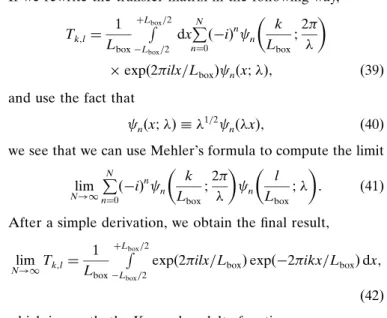
If we rewrite the transfer matrix in the following way,
Tk;l¼ 1 Lbox R þLbox=2 %Lbox=2 dxP N n¼0ð% iÞn n k Lbox ;2" ! ! "
,expð2"ilx=LboxÞ nðx;!Þ; ð39Þ
and use the fact that
nðx;!Þ +!
1=2
nð!xÞ; ð40Þ
we see that we can use Mehler’s formula to compute the limit lim N!1 PN n¼0ð% iÞn n k Lbox ;2" ! ! " n l Lbox ;! ! " : ð41Þ After a simple derivation, we obtain the final result,
lim N!1Tk;l¼ 1 Lbox R þLbox=2 %Lbox=2
expð2"ilx=LboxÞexpð%2"ikx=LboxÞdx; ð42Þ which is exactly the Kronecker delta function.
3.4. Encoding quality
There are several ways to evaluate the quality of a model encoding with the subsequent reconstruction. For example, in the optimal control theory (Boyd, 1991), the quality of a linear filter is estimated using a certain norm of the transfer matrix. However, in crystallography the most used quality criterion is the crystallographicRfactor (Stout & Jensen, 1968),
R¼ P l j ~ F Fexact l j%jFF~lmodj % % %% P l j ~ F Fexact l j ; ð43Þ
where FexactandFmod are the exact Fourier coefficients of a molecule and the coefficients computed from the Hermite coefficients, respectively. This quantity is a widely used measure of the agreement between a crystallographic model and the corresponding experimental X-ray diffraction data. In
Figure 7
AnalyticalRfactors in one dimension as a function of Hermite decomposition orderNand scaling parameter!computed at three different resolutions. The input signal is modelled as a sum of Gaussians (10) with a variance of#/21/2equispaced at a distance#. The number of Fourier coefficients isM= 30
and the input box size isLbox= 23.0 A˚ . These values were chosen to mimic the 1akg peptide decomposition. The estimate of the optimal parameter!(26)
is plotted as a red dashed line. The real-space bound on the optimal parameter!(22) is shown as an orange dashed line. The reciprocal-space bound on the optimal parameter!(24) is shown as a blue dashed line. Left, the Gaussian parameter#= 0.2 A˚ , corresponding to an absolute input signal resolution of"= 0.31 A˚ and a relative resolution"/Lbox= 0.014. However, in this case the actual absolute resolution is cut atLbox/M= 0.77 A˚ , which corresponds to
a relative resolution of 0.033. Middle, the Gaussian parameter#= 1.0 A˚ , corresponding to an absolute input signal resolution of"= 1.57 A˚ and a relative resolution"/Lbox= 0.068. Right, the Gaussian parameter#= 5.0 A˚ , corresponding to an absolute input signal resolution of"= 7.85 A˚ and a relative
the case of an ideal electron-density encoding, theRfactor is equal to zero. In protein crystallography, models with R
factors of less than 0.2 are regarded as good when working at a medium resolution.
The equations for the transfer matrix allow estimation of the R factor for certain classes of electron-density distribu-tions. As described above (10), we use the Gaussian distri-bution to model the electron density of an atom. Exact Fourier coefficients of a molecule withNatomsatoms at positionsriare
then given as ~ ffexactl;m;nðsÞ ¼# 3"3 2 P Natoms i¼1 expð%#2"2s2 lmnÞexpð%2i"rislmnÞ; ð44Þ
where sl,m,nis the wavevector and sl,m,n= (l/Lx, m/Ly, n/Lz),
whereLx,LyandLzare the dimensions of the bounding box
along the corresponding axes. Similarly, one-dimensional exact Fourier coefficients of the Gaussian function are given as
~
ffexactl ¼#"12 P
Natoms
i¼1
expð%#2l2=L2
boxÞexpð%2i"ril=LboxÞ: ð45Þ
To see how the Hermite basis encodes Gaussian densities with various level of detail, we built models of the electron-density map with different parameters#. The width of the Gaussian determines the resolution of the density map according to
"¼"#
2 : ð46Þ
The derivation of this formula follows the one well known in crystallography which describes the extinction of diffraction reflections. For the sake of completeness, we provide its derivation in AppendixC.
To estimate theRfactor for certain model parameters, we assume that the input electron density is given as a sum of Gaussians with variance of#/21/2equispaced at a distance#. Fig. 7 shows analyticalRfactors in one dimension computed using (33) and (45) as a function of the Hermite decomposi-tion order N and the scaling parameter !. We bounded the input and output frequencies byM= 30 Fourier coefficients. The size of the input intervalLboxis set to 23.0 A˚ to mimic the
#-conotoxin PnIB peptide (PDB entry 1akg) decomposition used in the fitting example below. We should stress that owing to the properties of the Hermite functions, the whole model is scale-invariant. More precisely, if we keep the product!Lbox
constant then the relative shape of the Hermite basis functions would not change. Also, if we scaleLboxand#simultaneously
then the value of theRfactor is unchanged. Therefore, it is useful to provide relative resolutions computed as "/Lbox.
Fig. 7 (left) showsRfactors for the Gaussian parameter#= 0.2 A˚ corresponding to an absolute input signal resolution of"
= 0.31 A˚ and a relative resolution"/Lbox= 0.014. However, in
this case the actual absolute resolution is cut at Lbox/M =
0.77 A˚ , which corresponds to a relative resolution of 0.033. Fig. 7 (middle) showsRfactors computed using the Gaussian parameter#= 1.0 A˚ corresponding to an absolute input signal resolution of " = 1.57 A˚ and a relative resolution "/Lbox =
0.068. Fig. 7 (right) shows R factors computed using the Gaussian parameter# = 5.0 A˚ corresponding to an absolute
input signal resolution of"= 7.85 A˚ and a relative resolution
"/Lbox = 0.34. The estimate of the optimal parameter!(26)
is plotted as a red dashed line. The real-space bound on the optimal parameter !(22) is shown as an orange dashed line. The reciprocal-space bound on the optimal parameter!(24) is shown as a blue dashed line. We see that on lowering the resolution of the input signal theRfactors decrease, as would be expected from general considerations. We can also see that the lower (22) and the upper (24) bounds on the optimal scaling parameter !follow the isolines of the R-factor map. Therefore, their mean given by (22) provides a reasonable estimation of the optimal value of!.
Fig. 8 showsRfactors as a function of input signal resolution
"for three different Hermite decomposition ordersN: 15, 20 and 30. Rfactors were estimated in the same way as in the previous case. More precisely, we assumed the same shape of the input electron density and then used (33) and (45) to compute the analyticalRfactors. For these plots, we computed the optimal scaling parameter ! using (22). The parameter
Lboxand the size of the transfer matrixMwere constant and
were equal to 23 A˚ and 30, respectively. As in the previous figure, these values are chosen to mimic the#-conotoxin PnIB peptide decomposition used in the fitting example below. The scale of the top horizontal axis gives the absolute resolution forLbox= 23 A˚ . The scale of the bottom horizontal axis gives
the relative resolution. In order to compute the absolute resolution, its values need to be multiplied by the chosen value of Lbox. As expected, the values of the Rfactors diminish as
the resolution becomes lower. This is because at low resolu-tions low-frequency columns of the transfer matrix become more important. In the limiting cases of zero and infinite resolutions, the Rfactor can be computed directly from the transfer matrix as a certain norm of T % I. For the infinite resolution limit, it is given as the L1 norm of the central
Figure 8
AnalyticalRfactors in one and three dimensions as a function of the relative resolution"/Lbox. The absolute resolution at box sizeLbox= 23 A˚
is shown on the top horizontal axis. Plots for three different Hermite expansions orders are shown;N2{15, 20, 30}. The parametersLboxandM
were constant and were 23 A˚ and 30, correspondingly. The scaling parameter!was estimated using (26).
column of the matrixT%I. For the zero resolution limit, the
R factor is given by the entry-wise L1 norm of T % I, R= P
i;jjTi;j%&i;jj. Fig. 8 also shows an estimation ofRfactors for
the three-dimensional case. It is based on the assumption that Hermite decomposition encoding in three dimensions behaves similarly to the one-dimensional case, with the number of coefficients scaled asN1D=N1/33D.
4. Results and discussion
We tested and verified our algorithm using two examples of different difficulty. The first example is the small polypeptide #-conotoxin PnIB. We generated the EDM for this example from the coordinates of the polypeptide. The second example is the fitting the GroEL domains into the electron-density map of the GroEL complex.
4.1.a-Conotoxin PnIB
Firstly, we explored the relationship between the encoding quality and the quality of the fitting. For this purpose, we chose the small 16-residue polypeptide#-conotoxin PnIB. We downloaded the X-ray crystal structure of#-conotoxin PnIB (PDB code 1akg; Huet al., 1997) from the PDB (Bermanet al., 2000) and simulated the electron-density map (2mFo%DFc)
using the Uppsala electron-density server (Kleywegt et al., 2004) with resolution " = 1.1 A˚ . We computed the protein density according to (10) with the Gaussian width#= 1.0 A˚ using only the non-H atoms of the standard amino acids. We rotated the initial 1akg structure by arbitrarily chosen Euler angles of’= 76-,$= 234-and = 56-and used it as the input
for the fitting workflow. We usedNrot= 500 (corresponding to
an angular step of 36-) rotations represented with uniformly
distributed Euler angles spanning the space 2",",2". The order of the Hermite expansion was set toN= 15, which is the minimum expansion order allowed at this resolution according to (28). The order of the Fourier expansion was twice the order of the Hermite expansion:M= 30 for each dimension.
To see how the encoding quality influences the fitting algorithm, we studied the dependence of the decomposition on the scaling parameter!. We chose a range of!parameters between 0.05 and 2.0. For each!, we computed the best fitting score along with the average fitting score. Fitting results are shown in Fig. 9. We see that by choosing a small!we neglect the details of the protein structure (Fig. 9a) and therefore we cannot discriminate between different orientations of the protein (the maximum score for!= 0.05 is very close to the average score). When choosing a sufficiently large!, we obtain satisfactory discriminative power to find the near-native position of the protein (Figs. 9cand 9d). We also see that, for example for!= 0.5, the difference between the maximum and the average score is much larger than in the case of!= 0.05. Also, when we take too large a!we cannot encode the whole protein (Fig. 9e). The red dashed line in Fig. 9 showsRfactors computed with (43). We see that the choice of the parameter! influences theRfactors and thus determines the quality of the
Figure 9
Test of the fitting algorithm on an artificially generated EDM for the
#-conotoxin PnIB (PDB entry 1akg). Here, we plotted the dependence of four parameters, the maximum score, the average score, the score of the near-native conformation and the crystallographicRfactor, on the scaling parameter !. The isosurface of the Hermite decomposition at protein model density equal to ('max+'min)/2 and several values of!are shown
in subplots A (!= 0.05), B (!= 0.15), C (!= 0.3), D (!= 0.55) and E (!= 2.0).
Figure 10
Result of fitting chain Aof the GroEL–GroES X-ray structure (PDB entry 1aon) to the GroEL complex electron-density map (EMD-2001). Two heptameric rings are shown in different colours. The average r.m.s.d. measured using the C#atoms between the two closest chains in the fitted
structure and the flexibly refined structure provided by the authors of the EDM (PDB entry 4aau) is 5.35 A˚ .
fitting. Notably, the minimum of the R-factor curve corre-sponds to the maximum of the fitting score.
Owing to the strong influence of the scaling parameter!on the discriminating power of the algorithm, we estimated its optimal value to gain the maximum separation between the score of the correct pose and the average score. Provided that the box that contains all of the rotations of the peptide has the sizeLbox= 23 A˚ and setting the resolution of the EDM"=
1.1 A˚ , (26) gives an estimate of the optimal value of the scaling parameter: !opt ’ 0.50. Fig. 9 shows that this estimation
corresponds to the best discrimination between the near-native and all other structures, which can be deduced from the maximum separation between the score of the prediction and the average score. The r.m.s.d. between the prediction and the solution at this value of!is 1.03 A˚ . We should note that the r.m.s.d can be decreased by taking a finer angular search step.
4.2. GroEL complex
Here, we demonstrate that our approach gives essentially the same results as other programs, provided that the scoring function is the same (LCCF in this case). For this purpose, we use a classical test for a fitting algorithm: the GroEL complex map. We downloaded the EDM of the GroEL complex from the Electron Microscopy Data Bank (EMDB; code EMD-2001) with a resolution of 8.5 A˚ . We then downloaded the crystal structure of the GroEL subunits from the PDB data-base. We used the GroEL–GroES complex structure (PDB entry 1aon; Xuet al., 1997), from which we extracted chainA, centred it and arbitrarily rotated it to exclude any bias. We chose the sampling grid size according to the resolution and the size of the EDM. The EDM was first padded with zeros and then transformed to the Fourier basis using the FFT
algorithm. The number of coefficients in the Fourier decom-positionMwas equal to 105,107,119. The angular search
step was set to 30-. We used a Hermite expansion order ofN=
15, which is larger than the minimum expansion order allowed at this resolution,Nmin’9 (see equation 28). We sampled the
rotations using the spiral algorithm (Saff & Kuijlaars, 1997), which generates an equispaced distribution of points on a sphere. Unlike in the previous example, owing to the lower resolution of the GroEL EDM, here we fitted Laplacian-filtered protein density into the Laplacian-Laplacian-filtered EDM.
After the six-dimensional exhaustive search, we clustered the solutions using a clustering threshold of 10 A˚ and kept the top 14 poses. All 14 poses corresponded to individual chains of the complex, which is comprised of two heptameric rings. Fig. 10 shows the results of the fitting. We compared the fitted model with the model provided by the authors of the EDM (PDB entry 4aau; Clareet al., 2012). The average r.m.s.d. between the chains owing to the flexible deformations measured using C# atoms was 3.0 A˚ . More precisely, we superposed the corresponding chains of both models using rigid-body transformations and then measured the r.m.s.d. between them. Overall, the average r.m.s.d. between C#atoms was 5.35 A˚ . This includes both the discrepancy between corresponding chains in the assembly arising from flexible deformations and the rigid-body misfit. The average distance between the centres of mass of the corresponding chains was 2.64 A˚ (Table 3).
4.3. Runtime of Hermite- to Fourier-space transition
The use of the fast Fourier transform has been an inevitable step in every fitting algorithm until now. Instead, we intro-duced a basis from which we can transform a decomposition into the Fourier basis avoiding evaluation of the FFT on a grid. When the grid becomes large, the asymptotic complexity of our algorithm becomes O(M3N) (see equation 21). It is
comparable to the complexity of the fast Fourier transform
Table 2
Comparison of theHermiteFitalgorithm with thecoloresandADP_EM
algorithms.
The comparison criteria were chosen to be the total running time and the running time per point of search space
Algorithm No. of rotation-space points No. of translation-space points Runtime (s)
Time per point (,10%7s)
ADP_EM 16384 23186 139 3.6
colores 4416 1336965 1454 2.5
HermiteFit 4416 1336965 917 1.5
Table 3
Comparison of the models obtained using theHermiteFit,colores and
ADP_EM algorithms with the model obtained by the authors of the electron-density map (PDB entry 4aau).
For each pair of models, the r.m.s.d. was measured using the C#atoms and the
centres of mass of the corresponding chains and was then averaged over all of the chains comprising the assembly.
Algorithm R.m.s.d., C#(A˚ ) R.m.s.d., centres of mass (A˚ )
ADP_EM 4.61 2.29
colores 5.42 2.52
HermiteFit 5.35 2.64
Figure 11
Running times of the Hermite-to-Fourier space transition performed using our algorithm and theFFTalgorithm on a cubic grid ofM,M,M
as a function of the Fourier expansion orderM. We used the FFTW3 library (Frigo & Johnson, 2005) with the double-precision real discrete Fourier transform using the flag FFTW_ESTIMATE to measure the speed of the FFT. The order of the Hermite expansion wasN= 15.
algorithm, O(M3logM). Intuitively, at large orders of the Fourier expansionMour algorithm should be faster compared with the FFT. Thus, we conducted a numerical experiment to compare the actual running times. Fig. 11 shows the time needed to compute the FFT on a cubic grid of sizeMand the time needed to transform a Hermite expansion of orderN= 15 to the same Fourier grid. We can see that, generally, at large values ofM,M>.100, the transition from Hermite space into Fourier space is faster compared with the speed of the FFT. Also, the timing of the transition grows evenly with respect to
Min contrast to the timing of the FFT. One has to take into account that we compared our algorithm with the highly optimized FFTW3 library (Frigo & Johnson, 2005). It is probable that additional optimization of HermiteFit could improve performance even further. One of the ways to speed up the transition will be to use the fast Hermite transform instead of naive matrix multiplication (Leibon et al., 2008). This implementation will be the subject of future work.
4.4. Comparison withSitusandADP_EM
We compared the HermiteFit algorithm with two popular existing fitting methods: the coloresprogram from the Situs
package (Chaco´n & Wriggers, 2002) and theADP_EMfitting tool (Garzo´net al., 2007). These two packages represent the two major approaches to the problem of exhaustive search in six-dimensional space of rigid-body motions.Colores, a widely used CCF-based fitting tool, rapidly scans the translational degrees of freedom using the fast Fourier transform. The rotations, however, are sampled exhaustively by enumerating a list of equispaced distributed rotations on a sphere.
ADP_EM choses points in real space, places the atomic
structure there and then rotationally matches it to the EDM using the fast rotational matching algorithm. The authors of
ADP_EM compared their algorithm with five-dimensional
rotational matching and found that three-dimensional rota-tional matching works faster in practice (Garzo´net al., 2007). For comparison, we normalized the running times of the fitting algorithms by the sizes of the search space. Forcolores
and HermiteFit the size of the search space is equal to the number of grid cells (M3 for a cubic grid in theHermiteFit
algorithm) multiplied by the number of sampled angles. The size of the search space of the ADP_EM algorithm is the number of points in real space times the number of cells of the angular grid. The latter is built from uniformly sampled Euler angles on a grid of 2",",2". The size of the angular grid is determined by the order Nexp of a spherical harmonics
expansion and equals 4N3exp. For coloresandHermiteFit, we
used an angular search step of 30-. The resolution of the EDM
forcoloresandHermiteFitwas set to 8.5 A˚ . The Fourier grid that was used by colores and the HermiteFit algorithm had dimensions of 105 , 107 , 119. For ADP_EM, we used a spherical harmonics expansion order ofNexp= 16.
Table 2 shows the normalized times of the complete six-dimensional search for the three algorithms in the case of fitting the GroEL subunit into the 8.5 A˚ resolution GroEL electron-density map. Judging by the total running time,
ADP_EM has a large advantage over the two other
algo-rithms, which exhaustively search all of the space of possible translations. However, in terms of running time per search point, the HermiteFit algorithm is more effective than the other two. Interestingly,coloresspends about half of the total search time on computation of the Fourier coefficients of the rotated protein. Therefore, it was very important for us to speed up this step. Nonetheless, all three tested algorithms have their own advantages and drawbacks. For example,
ADP_EM can use smart heuristics to reduce the number of search points in real space. However, its sample points in the space of rigid-body rotations are distributed non-uniformly. In particular, rotations near the poles are sampled more densely, making this sampling scheme less effective (Saff & Kuijlaars, 1997). On the other hand, theHermiteFitalgorithm along with the colores algorithm sample the rotational space nearly uniformly using the spiral algorithm while the translational space sampling also remains uniform. We would like to stress that the absolute runtimes (shown in Table 2) are not very informative. In particular, they dramatically depend on the choice of the FFT library, code optimization, the choice of compiler and compilation optionsetc. However, this compar-ison clearly demonstrates that the new approach paves the way to speed up one of the bottlenecks of fitting methods: the projection of the rotated structure into the Fourier space.
To assess the fitting quality of the tested methods, we measured the r.m.s.d.s between the obtained models and the structure obtained by the authors of the electron-density map (PDB entry 4aau). Table 3 shows a comparison of the measured r.m.s.d.s forADP_EM,coloresandHermiteFit. We used two different criteria for the measurements. Firstly, we measured the average r.m.s.d. between C#atoms. Secondly, we measured the average distance between the centres of mass of the corresponding chains. ADP_EM produced a model with an r.m.s.d. of 4.61 A˚ from the solution; the r.m.s.d.s forcolores
and HermiteFit were 5.42 and 5.35 A˚ , respectively. Clearly, Table 3 demonstrates that the tested algorithms produce equal quality models. However, the results ofADP_EMare slightly better, presumably because of the finer rotational sampling.
5. Conclusion
In this paper, we have presented HermiteFit, a new method that performs an exhaustive search in the six-dimensional space of rigid-body motions. It uses orthogonal Hermite functions to encode the electron density and performs the critical steps of the fitting workflow in Hermite space. As part of the new method, we developed an algorithm for the rota-tion of the decomposirota-tion in the Hermite basis and an algo-rithm for the conversion of the Hermite expansion coefficients into the Fourier basis. By introducing the Hermite decom-position into the EDM fitting workflow, we inevitably intro-duced an additional scaling parameter!. For this parameter, we provided tight bounds and an estimation of the optimal value that depends only on the properties of the fitting problem and the desired order of the polynomial decom-position (equations 25 and 26). Using two examples, we
demonstrated the validity of these bounds as well as the sufficiency of the Hermite expansion of orderN= 15 to solve the standard EDM fitting problems. In particular, we derived a formula for Laplacian-filtered Hermite decomposition and employed this result to fit a single chain of GroEL into its electron-density map. Using analytical analysis, we calculated the crystallographicRfactor produced by our method, which does not depend on the particular density that we encode. This allowed us to avoid tuning of fitting parameters and provided a clear understanding of the error sources in the algorithm. Finally, we compared our algorithm with two widely used fitting methods:ADP_EMandcoloresfrom theSituspackage. The proposed algorithm can be straightforwardly applied to other problems in structural bioinformatics such as, for example, protein–protein and protein–ligand docking. It can also be used for computer vision and three-dimensional object-recognition problems. The improvement in the speed of the algorithm may have an impact on flexible protein docking, flexible EDM fitting and other difficult problems that require a six-dimensional exhaustive space search as their initial step.
HermiteFit will be made available stand-alone at http:// nano-d.inrialpes.fr/software/HermiteFit and as a plugin for the
SAMSON software platform, and is available upon request from the authors.
APPENDIXA
Shifted Gaussian expansion
Here, we provide the derivation of the expansion coefficients of a shifted Gaussian of the form
gðrÞ ¼exp %jr%r0j
2
#2
! "
ð47Þ into the orthogonal Hermite basis. The well known property of this basis (as well as of any orthogonal basis) is the following:
iffðx;y;zÞ ¼fð1ÞðxÞfð2ÞðyÞfð3ÞðzÞ andfðkÞðtÞ ¼PN i¼0 ^ ffiðkÞ iðt;!Þ then ^ ffi;j;k¼ff^ið1Þff^jð2Þff^kð3Þ: ð48Þ Firstly, we derive the decomposition of a one-dimensional Gaussian into the one-dimensional orthogonal Hermite basis. Then, using property (48), we obtain the decomposition of a three-dimensional Gaussian into the three-dimensional orthogonal Hermite basis. More specifically, the one-dimensional Gaussian function is
gðxÞ ¼exp %ðx%%Þ
2
#2
# $
: ð49Þ
Its decomposition coefficients are
^ ggnð%;!;#Þ ¼ R gðxÞ nðx;!Þdx ¼ n!!1=2exp %% 2 #2 1% 1 #2(2 ! " # $ ð2nn!"1=2Þ1=2 P ðn=2Þ m¼0 ð%1Þm m!ðn%2mÞ! ð50Þ ,Rexp %(2 x %#2%(2 ! "2 " # 2! x% % #2(2 ! " þ#22!%(2 # $n%2m dx
where(2= (!2/2) + (1/#2). From now on, we will, for brevity,
writegg^ninstead ofgg^nð%;!;#Þ. Changing the variablest=x%
(%/#2(2) and denotinga=%/#2(2, we obtain
^ ggn¼ n!!1=2 exp %% 2 #2 1% 1 (2 ! " # $ ð2nn!"1=2Þ1=2 P ðn=2Þ m¼0 ð%1Þmð2!Þn%2m m!ðn%2mÞ! , Rexpð%(2t2 ÞðtþaÞn%2mdx: ð51Þ Next, we decompose the sum (t+a)kusing Newton’s formula,
ðtþaÞk¼P k i¼0 k i ! " tiak%i: ð52Þ Thus, the integral in (51) will read
R expð%(2t2 ÞðtþaÞn%2mdx ¼ P n%2m i¼0;i-even ðn%2mÞ! 2iði=2Þ!ðn%2m%iÞ!" 1=2(%1%ian%2m%i: ð53Þ Substituting it into the formula forgg^nnand denoting
Pn%2m
i¼0;i-even
=P½ðl¼n0%2mÞ=2&(i= 2l), we obtain the following expression for the coefficients, ^ ggnð%;!;#Þ ¼exp % %2 #2 1% 1 #2(2 ! " # $ n!"1=2! 2n ! "1=2 ,ðP n=2Þ m¼0 P ½ðn%2mÞ=2& l¼0 ð%1Þm2n%2m%2l!n%2m l!ðn%2m%2lÞ!m! (% 2nþ4mþ2l%1 % #2 ! "n%2m%2l : ð54Þ Finally, using (48) we obtain a decomposition of the three-dimensional Gaussian into the three-three-dimensional Hermite basis. We should note that in order to avoid the rounding error, one should begin the summation with the Gaussians that are located farther from the origin.
APPENDIXB
Fast summation
Here we explain the fast summation in (55),
~ ffl;m;n¼ PN i¼0 P N%j j¼0 P N%i%j k¼0 ^ ffi;j;k~i;l~j;m~k;n; ð55Þ
with indices l,m,n2(0,M). The summation in this formula can be performed with less operations than a naive estimation
O(M3N3) suggests. We perform the fast summation by splitting
the equation into three consecutive sums:
g T1 i;j;n T1 i;j;n¼ P N%i%j k¼0 ^ ffi;j;k~k;n; ð56Þ