Notes on Power System Load Flow Analysis using an Excel Workbook Abstract
These notes describe the features of an MS-Excel Workbook which illustrates four methods of power system load flow analysis. Iterative techniques are represented by the Newton-Raphson and Gauss-Seidel methods. The Workbook also includes two search algorithms: genetic algorithms and simulated annealing.
1. Introduction
Load flow studies [1,2] are used to ensure that electrical power transfer from generators to consumers through the grid system is stable, reliable and economic. Conventional techniques for solving the load flow problem are iterative, using the Newton-Raphson or the Gauss-Seidel methods. Recently, however, there has been much interest in the application of stochastic search methods, such as Genetic Algorithms [3,4,5], to solving power system problems. The increasing presence of distributed alternative energy sources, often in geographically remote locations, complicates load flow studies and has triggered a resurgence of interest in the topic. The principles of power system load flow studies are taught within elective modules in the later years of undergraduate electrical engineering courses, or as essential components of specialist masters programmes in electrical power engineering. From the educational viewpoint, therefore, the topic is important, yet a complete coverage presents some significant challenges. Pre-requisites include fundamental concepts from a.c. circuit analysis, such as phasor notation, impedance and admittance, power and reactive power, three-phase and per-unit systems, all of which are regarded as ‘difficult’ by many students. The load flow solution techniques bring extra mathematical hurdles, including matrix representation (with complex number coefficients), iterative methods and probability functions.
To assist in the teaching of load flow analysis techniques the Excel Workbook illustrates four different methods of solving a simple load flow problem, which nevertheless has all of the features to be found in a larger-scale system. The Workbook allows students to vary both the problem being solved, by adjusting the power or voltage levels and line impedances, and also the parameters of the solution methods, such as numerical acceleration factors. These notes present an overview
of the general power system load flow problem and describe its solution using four techniques: Newton-Raphson, Gauss-Seidel, Genetic Algorithm and Simulated Annealing. Also included are illustrative numerical results relating to the particular power system configuration analysed in the Workbook.
2. Formulation of the Load Flow Problem
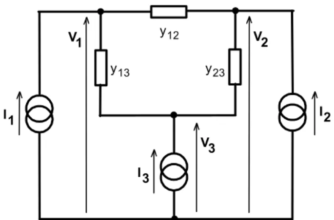
Load flow studies are based on a nodal voltage analysis of a power system. As an example, consider the very simple system represented by the single-line diagram in Fig. 1. Here two generators (1 and 2) are interconnected by one transmission line and are separately connected to a load (3) by two other lines. If the phasor currents injected into the system are I1, I2, and I3, and the lines are modelled by simple series
admittances, then it is possible to draw the equivalent circuit for one representative phase of the balanced three-phase system, as shown in Fig. 2.
generator, 1 generator, 2
load, 3
Fig. 1 Single-line diagram of a simple example power system
V1 y12 I1 I2 I3 V2 y13 y23 V3
Fig. 2 Equivalent circuit for one phase of the system shown in Fig.1
For the circuit in Fig. 2 the nodal voltage equations can be written directly. For example, at node 1:
(
)
1 2 31 V V V
I = y12+y13 −y12 −y13 (1)
In general, for a system with r nodes, then at node n:
∑
= = + + + + + = r k nk nr nn n n Y Y Y Y Y 1 2 1 1 2 ... n ... r k n V V V V V I (2)where: Ynn = sum of all admittances connected to node n
Ynk = - (sum of all admittances connected between nodes n and k) = Ykn
In= current injected at node n
= r n 1 r n 1 V : V : V I : I : I . .. .. : : : .. .. : : : .. .. 1 1 1 1 11 rr rn r nr nn n r n Y Y Y Y Y Y Y Y Y or
[ ] [ ][ ]
I = Y .V (3)where [Y] is the nodal admittance matrix. Formulation of the load flow problem is most conveniently carried out with the terms in the nodal admittance matrix expressed in polar notation: Ykn = Ykn∠θkn. The Excel Workbook (Sheet 2) allows users to enter series impedance data for the three lines and then automatically calculates the terms in the nodal admittance matrix.
Conventional circuit analysis proceeds directly from equation (3) by inverting the nodal admittance matrix and hence solving for the nodal voltages [V]. However, the load flow problem is complicated by the lack of uniformity in the data about electrical conditions at the nodes. There are three distinct types of nodal data, which relate to the physical nature of the power system:
a) Load nodes, where complex power Sns= Pns +jQns taken from or injected into the
system is defined. Such nodes may also include links to other systems. At these load nodes, the voltage magnitude |Vn| and phase angle δn must be
calculated.
b) Generator nodes, where the injected power, Pns, and the magnitude of the nodal
voltage |Vn| are specified. These constraints reflect the generator’s operating
characteristics, in which power is controlled by the governor and terminal voltage is controlled by the automatic voltage regulator. At the generator nodes the voltage phase angle δn must be calculated
c) At least one node, termed the ‘floating bus’ or ‘slack bus’, where the nodal voltage magnitude |Vn| and phase angle δn are specified. This node acts as the
reference node and is commonly chosen to have a phase angle δn = 0o. The
power and reactive power delivered at this node are not specified.
In the system configuration of Fig. 1, which is analysed in the Excel Workbook, each type of node is represented with node 1 being a floating bus, node 2 being a generator node and node 3 being a load node. Consequently values must be specified for the power (P2s) injected at node 2, and the power (P3s) and reactive
power (Q3s) injected at node 3. All three of these power values may be changed by
the user, though default values are provided (P2s = 1.0; P3s = -1.5; Q3s = -0.2), with
negative values indicating that power or reactive power is being drawn from the system. The magnitude of the voltage at node 1 can be specified, with the default value being 1.0 pu, while the phase angle is fixed at 0o ( =1.0∠00
1
V ). At the generator node (node 2), the voltage magnitude can be set by the user with the default value being 1.1 pu (V2 =1.1∠δ2),and the phase angle δ2 is calculated during
the load flow solution. At the load node (node 3) the voltage magnitude and phase angle have to be calculated (V3 =V3∠δ3). So the complete load flow problem for this particular power system configuration involves the calculation of the voltage magnitude V3 and the phase angles δ2,δ3.
3. Newton Raphson Method 3.1. General Approach
The Newton-Raphson method is an iterative technique for solving systems of simultaneous equations in the general form:
r r n n n r n j r n K x x x f K x x x f K x x x f = = = ) ,.. ,.. ( ) ,.. ,.. ( ) ,.. ,.. ( 1 1 1 1 1 (4)
where f1,....fn....fr are differentiable functions of the variables x1,....xn ,....xr and K1,
....Kn....Kr are constants. Applied to the load flow problem, the variables are the nodal
voltage magnitudes and phase angles, the functions are the relationships between power, reactive power and node voltages, while the constants are the specified values of power and reactive power at the generator and load nodes.
Power and reactive power functions can be derived by starting from the general expression for injected current (Eqn. 2) at node n:
∑
= = r k nk Y 1 k n V Iso the complex power input to the system at node n is:
*
n n
n V I
where the superscript * denotes the complex conjugate. Substituting from (2) with all complex variables written in polar form:
{
n k nk}
r k nk k n r k k nk n n =∑
Y =∑
V V Y ∠δ −δ −θ = =1 1 * *V V S (6)The power and reactive power inputs at node n are derived by taking the real and imaginary parts of the complex power:
{ }
{
n k nk}
r k nk k n n n V V Y P =ℜ =∑
δ −δ −θ = cos 1 S (7){ }
{
n k nk}
r k nk k n n n V V Y Q =ℑ =∑
δ −δ −θ = sin 1 S (8)The load flow problem is to find values of voltage magnitude and phase angle, which, when substituted into (7) and (8), produce values of power and reactive power equal to the specified set values at that node, Pns and Qns.
The first step in the solution is to make initial estimates of all the variables: 0, 0
n n
V δ where the superscript 0 indicates the number of iterative cycles completed. Using these estimates, the power and reactive power input at each node can be calculated from (7) and (8). These values are compared with the specified values to give a power and reactive power error. For node n:
{
n k nk}
r k nk k n ns n P V V Y P = − δ −δ −θ ∆∑
= 0 0 1 0 0 0 cos (9){
n k nk}
r k nk k n ns n Q V V Y Q = − δ −δ −θ ∆∑
= 0 0 1 0 0 0 sin (10)The power and reactive power errors at each node are related to the errors in the voltage magnitudes and phase angles, e.g. 0, 0
n n
V ∆δ
∆ , by the first order approximations: ∆ ∆ ∆ − − − ∆ ∆ ∆ − − − − − − − − − − − − − − − − − − − − − − − − − = ∆ − − − ∆ + − + − + − + − + − + − 0 1 0 0 1 0 1 0 0 1 1 1 1 1 1 1 1 1 0 0 . : : : : : : : : : : : : : : : : : : : : : : : : : : : : : : : : : : : : : : : : : : : : : : : : : : : : : : : : : : n n n n n n n n n n n n n n n n n n n n n n n n n n n n n n n n V V V V Q V Q V Q Q Q Q V P V P V P P P P Q P δ δ δ ∂ ∂ ∂ ∂ ∂ ∂ ∂δ ∂ ∂δ ∂ ∂δ ∂ ∂ ∂ ∂ ∂ ∂ ∂ ∂δ ∂ ∂δ ∂ ∂δ ∂ (11)
where the matrix of partial differentials is called the Jacobian matrix, [J]. The elements of the Jacobian are calculated by differentiating the power and reactive power expressions (7,8) and substituting the estimated values of voltage magnitude and phase angle.
At the next stage of the Newton-Raphson solution, the Jacobian is inverted. Matrix inversion is a computationally-complex task with the resources of time and storage increasing rapidly with the order of [J]. This requirement for matrix inversion is a major drawback of the Newton-Raphson method of load flow analysis for large-scale power systems. However, with the inversion completed, the approximate errors in voltage magnitudes and phase angles can be calculated by pre-multiplying both sides of (11): ∆ − − − ∆ − = ∆ ∆ ∆ − − − ∆ ∆ ∆ + − + − : : : : . 1 0 0 0 0 1 0 0 1 0 1 0 0 1 n n n n n n n n Q P V V V
J
δ δ δ (12)The approximate errors from (12) are added to the initial estimates to produce new estimated values of node voltage magnitude and angle. For node n:
0 0 1 n n n V V V = +∆ (13) 1 0 0 n n n δ δ δ = +∆ (14)
Because first-order approximations are used in (11) the new estimates (denoted by the superscript 1) are not exact solutions to the problem. However, they can be used in another iterative cycle, involving the solution of Equations (9-14). The process is repeated until the differences between successive estimates are within an acceptable tolerance band.
The description above relates specifically to a load node, where there are two unknowns (the voltage magnitude and angle) and two equations relating to the specified power and reactive power. For a generator node the voltage magnitude Vn and power Pn are specified, but the reactive power is not specified. The order of the calculation can be reduced by 1. There is no need to ensure that the reactive power is at a set value and only the angle of the node voltage needs to be calculated, so
one row and column are removed from the Jacobian. For the floating bus, both voltage magnitude and angle are specified, so there is no need to calculate these quantities.
3.2. Application of the Newton-Raphson Method to the Specific Problem
For the example system shown in Fig. 1 and analysed in the Excel Workbook, there are three unknowns (V3,δ2,δ3) and three set values of power and reactive power (P2s, P3s, Q3s). General expressions for power and reactive power input at nodes 2
and 3 can be derived from (7) and (8):
{
}
22{
22}
2 3 23{
2 3 23}
2 2 21 1 2 21 1 22 =V V Y cosδ −δ −θ +V Y cos−θ +V V Y cosδ −δ −θ
P (15)
{
}
{
}
33{
33}
2 3 32 2 3 32 2 3 31 1 3 31 1 33 =V V Y cosδ −δ −θ + V V Y cosδ −δ −θ +V Y cos −θ
P (16)
{
}
{
}
33{
33}
2 3 32 2 3 32 2 3 31 1 3 31 1 33 =V V Y sinδ −δ −θ +V V Y sinδ −δ −θ +V Y sin −θ
Q (17)
In the iterative solution process, (15-17) are used to calculate the power and reactive power inputs from latest estimates of node voltages and then using (9,10) to calculate the power errors. The terms in the Jacobian are obtained by partial differentiation of (15-17). For example:
{
3 1 31}
2 32{
3 2 32}
3 33{
33}
311 3
3 = cosδ −δ −θ + cosδ −δ −θ +2 cos −θ ∂ ∂ V Y V Y V Y V P (18)
{
3 2 32}
32 2 3 2 3 sinδ δ θ δ = − − ∂ ∂P V V Y (19) Inversion of the 3x3 Jacobian with scalar elements is easily accomplished in Excel. (12) can be used to derive the approximate errors in the three variables and new estimates formed from (13,14). These new estimates are applied in the subsequent iterative cycle.3.3. Sample Results for the Newton-Raphson Method
For the default system inputs, defined in Section 2, the Newton-Raphson method, implemented in the 3rd sheet of the Excel Workbook, produces the results shown in
Table 1. In this simple example, only 5 iterations are needed to generate results which are stable to three decimal places, even though the initial estimates of all three unknowns are far from the correct value. When making comparisons with other methods of solution, it is important to realise that each iterative cycle of the
Newton-Raphson method involves considerable computational effort, notably to invert the Jacobian.
4. Gauss-Seidel Method 4.1. General Approach
The Gauss-Seidel Method is another iterative technique for solving the load flow problem, by successive estimation of the node voltages. Equation (2) can be re-arranged to give an expression for the complex conjugate of the current input at node n:
∑
∑
+ = − = + + = r n k nk nn n k nk Y Y Y 1 1 1 * k * * n * * k * * n V V V I (20) Substituting for * n I from (20) into (5):∑
∑
+ = − = + + = r n k nk nn n k nk n n Y Y Y 1 1 1 * k * * n * * k *V V V V S (21) and re-arranging: * * * k * * * k * * n V S V V V nn n n r n k nn nk n k nn nk Y Y Y Y Y + − − =∑
∑
+ = − = 1 1 1 (22) The node voltage Vn appears on both sides of (22), which cannot, therefore, be used to give a direct solution. However, this equation is used in the Gauss-Seidel method as the basis for an iterative solution. If pn
V and p+1
n
V denote the values of the voltage at node n after p and p+1 iteration cycles, (22) can be written:
* n * *(p) k * * 1) *(p k * 1) (p * n V S V V V nn p n r n k nn nk n k nn nk Y Y Y Y Y ) ( 1 1 1 + − − =
∑
∑
+ = − = + + (23)Note that in evaluating the nth node voltage, the latest estimates of the other node voltages are used. In the p+1th iteration cycle when performing the calculation for node n, the voltages at the nodes k=1…n-1 are available, but for the other node voltages the values from the previous (pth) cycle have to be used.
The foregoing discussion is appropriate to load nodes. At the floating bus the voltage
n
V is known and so does not need to be calculated. Generator nodes are particularly problematical for the Gauss-Seidel Method. At these nodes the power Pn and voltage
magnitude Vn are specified, so in (23) p+1
n
imaginary part of Sn) is unknown. This difficulty is addressed by first calculating Qn,
as follows:
the voltage component:
(
)
*n * *(p) k * * 1) *(p k * 1) (p * n V V V V nn p n r n k nn nk n k nn nk Y P Y Y Y Y ) ( 1 1 1 # + − − =
∑
∑
+ = − = + + (24)can be calculated immediately and substituted into (23):
(
)
* n 1) (p * n 1) (p * n V V V nn p n Y jQ ) ( # + = + + (25)but, for a generator node, the magnitude Vn is known, so considering the magnitudes in (25):
(
)
(
)
+ ℑ + + ℜ = + + 2 ) ( # 2 ) ( # 2 * n 1) (p * n * n 1) (p * n V V V V nn p n nn p n n Y jQ Y jQ V (26)which can be solved for Qn (by iteration if necessary). The calculated value of Qn is
substituted back into (25) and the new estimate of generator node voltage is found. When compared to the Newton-Raphson Method, the Gauss-Seidel Method involves simple calculations, but is slow to converge. Therefore, it is common practice to accelerate the iterative process, by adding to the newly-calculated value of each variable an extra term proportional to the difference between the new and previous values. For example:
{
*(p)}
n 1) *(p n 1) *(p n 1) *(p n V V V V + = + +α. + − d accelerate (27)where α is an ‘acceleration factor’, which has a typical value of 0.6. 4.2. Application of the Gauss-Seidel Method to the Specific Problem
For the particular 3-node problem, introduced in Section 2, Equation (23) can be used directly to calculate the voltage at the load node (node 3) every iterative cycle. To deal with the generator node (node 2), multiply (25), with n=2, by *
2 V(p)Y22:
(
)
2 # 22 ) ( 22 ) (pY + = pY *(p+1) + jQ 2 * 2 1) (p * 2 * 2 V V V V (28)and expressing the phasor voltages in polar form:
2 # 2 22 22 2 1 2 22 22 2 Y V V Y V jQ V ∠ ∠− ∠− + = ∠ ∠− ∠ # + 2 p 2 p 2 p 2 θ δ δ θ δ δ (29)
the term jQ2 is imaginary and can be eliminated by equating real parts in (29):
} cos{ } cos{ # 22 2 22 2 22 1 2 22 2 Y V δ2p −δ2p+ −θ = V Y V δ2p +δ2# −θ V (30) } cos{ } cos{ # 22 2 22 1 2 δ −δ −θ = δ +δ −θ ∴ + # 2 p 2 p 2 p 2 V V (31)
− + − − = ∴ + arccos cos{ } 22 2 # 2 22 1 δ θ δ δ θ δ # 2 p 2 p 2 p 2 V V (32)
4.3. Sample Results for the Gauss-Seidel Method
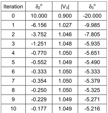
The Gauss-Seidel Method, defined by (23,24,25,27,32), for solving the load flow problem outlined in Section 2 is implemented in Sheet 4 of the Excel Workbook. Sample results for the default input data and using an acceleration factor α = 0.6 are shown in Table 2.
Comparing the results from Table 2 with those from Table 1, the slower convergence of the Gauss-Seidel Method is evident: even after 10 iteration cycles the values of phase angle are stabilised only to a single decimal place. However the computational effort involved in each cycle is much reduced in the Gauss-Seidel Method. Nevertheless both iterative methods require some complicated mathematical operations: inversion of the large Jacobian matrix in the Newton-Raphson Method and intermediate calculation of reactive power input at generator nodes in the Gauss-Seidel Method.
5. Stochastic Search Techniques 5.1. General Principles
Recent developments in load flow analysis have moved attention away from the iterative methods and towards so-called stochastic search methods. Two such methods – Genetic Algorithms and Simulated Annealing – are described here and are implemented in the Excel Workbook. Both approaches use a series of trial solutions to the problem and develop better solutions in the light of experience gained from these trials. The computational effort for each trial is kept as low as possible, so a very large number of trials can be conducted.
For the example problem being considered throughout this paper, there are three variables: the voltage magnitude V3 and the phase angles δ2,δ3. In any one trial some appropriate values are chosen for these variables. The choice may be an entirely random selection across the entire possible range of values (termed the ‘search space’) or the choice may be informed by previous experience. Once these trial values are chosen, the phasor voltages at all three nodes are defined, because all of the other voltage magnitudes and phase angles are fixed. Therefore the
currents injected at each node can be evaluated directly using (2) and the corresponding complex power input is calculated using (5).
The success of the trial needs to be judged by some quantitative criterion. The trial values of node voltage lead to values of input power and reactive power (P, Q) that do not exactly match the pre-defined values (Ps, Qs). The extent of the mis-match
can be quantified conveniently, for this particular problem, with the error function:
2 3 3 2 3 3 2 2 2 ) ( ) ( ) (P Ps P Ps Q Q s E = − + − + − (33)
The stochastic search techniques use the error function to inform the selection of new potential solutions for the subsequent round of trials. It is this selection process which is defined by the particular search technique.
5.2. Genetic Algorithms
Genetic Algorithms imitate the process of evolution, where the fittest individuals are likely to survive in a competing environment. A genetic algorithm [3,4] starts with a random population of potential individuals, or chromosomes, each representing one possible solution to a problem. The chromosomes are simply a collection of genes, each gene being one of the solution variables. The chromosomes are then evolved through successive generations. During each generation, all the chromosomes are evaluated, according to a defined fitness criterion, and the best chromosomes are selected to mate and generate offspring. The least fit chromosomes of each population are then replaced by the offspring so that the population size remains constant. After several generations, the algorithm converges to the best chromosome which represents an optimal solution to the problem.
A further refinement of the evolution process, again mirroring nature, is that any chromosome in any generation has a finite probability of suffering mutation, in which some of the genes are randomly perturbed. It is this process which ensures that the genetic algorithm does not converge to a local minimum when searching for a global problem solution.
When applied to the load flow problem, the genes are the nodal voltage magnitude and phase angle values and each chromosome contains a complete set of the genes needed to define uniquely a trial solution. The fitness of each chromosome is evaluated using the error criterion (33), which is used as the basis of selection for the
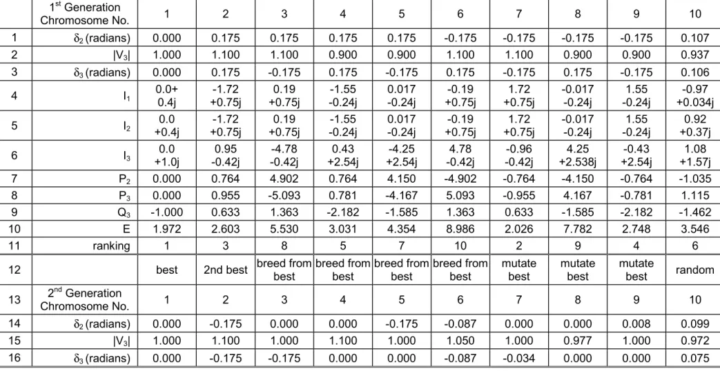
chromosomes in the next generation. For the example problem, a genetic algorithm solution is implemented in Sheet 5 of the Excel Workbook. Results from the common example problem during the early stages of the algorithm are shown in Table 3. An initial population of 10 chromosomes forms the first generation. Chromosome 1 is placed at the centre of the search space, chromosomes 2-9 are located at the extremes of the search space and chromosome 10 has random values. The values of the genes, voltage magnitude V3 and the phase angles δ2,δ3, for each chromosome are shown in rows 1-3 of the Table. Each chromosome, in association with the pre-defined values of V1 ,V2 and δ1, defines a set of trial nodal voltages, which are used to calculate the input currents (rows 4-6) and the power / reactive power inputs (rows 7-9). The set values for the power inputs are (P2s = 1.0; P3s =
-0.5; Q3s = -0.2), and the error function defined in (33) is evaluated for each
chromosome at row 10 with a low value of error function indicating a closer match between the calculated and set power values. The chromosomes are then ranked (row 11) by error. Rows 1-11 represent one complete generation of the genetic algorithm’s evolutionary process.
Chromosomes for the second generation are derived from the previous generation’s chromosomes according to their ranking. Row 12 indicates how each chromosome in the second generation has been formed. The first two chromosomes are copies of the two highest-ranked chromosomes of the previous generation. Chromosomes 3-5 are obtained by breeding between chromosomes 1 and 2: in each case one gene in chromosome 1 is replaced by the corresponding gene from chromosome 2. Each gene in chromosome 6 takes the average value of the genes in chromosomes 1 and 2. Mutation takes place in chromosomes 7-9, with one gene in turn from chromosome 1 being replaced by a random value. Finally, chromosome 10 of the second generation has genes which are entirely randomly-selected. So the new generation has 10 chromosomes, most of which are related to the best chromosomes from the previous generation.
The cycle of chromosome evaluation and breeding continues through many generations. Evaluation of the error function for each chromosome requires relatively simple calculations, so the genetic algorithm can continue through many generations until the error has fallen to acceptable levels. A typical variation of error with generation number is shown in Fig. 3. The genetic algorithm quickly reduces the error, but a very large number of generations is needed to bring the error close to zero. In the Excel Workbook, accelerated convergence is obtained after 100 generations, by redefining the search space so that it is centred on the best available solution at that stage and is reduced in size. The effect of this redefinition is apparent in Fig. 3, where the error reduction receives fresh impetus after the 100th generation.
5.3 Simulated Annealing
Simulated annealing is a global search technique in which a randomly-generated potential solution, Y, to a problem is compared to an existing solution, X. The probability of Y being accepted for investigation depends on the proximity of Y to X and the extent to which the solution has been developed, as represented by a ‘temperature’ parameter, T, which reduces throughout the annealing process. Both potential solutions are investigated and Y is chosen to replace X as the existing
0.0 0.5 1.0 1.5 2.0 0 50 100 150 200 e rro r number of generations Fig. 3 Typical error associated with the best chromosome as a function
solution according to a probability function, which again depends on the temperature T.
To apply this concept to load flow studies in general, it is assumed that the solutions X and, Y, represent information about possible nodal voltage values. In the particular illustrative example defined in Section 2, there are three unknown voltage values, so the solutions can be written:
[
X,V X, X]
Y[
Y,V Y, Y]
X =
δ
2 3δ
3 =δ
2 3δ
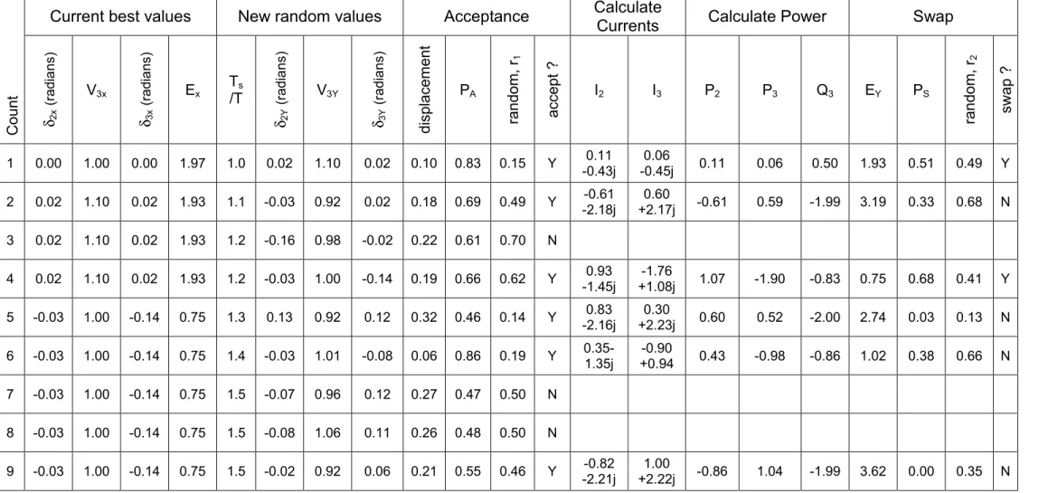
3 (34)where these solutions must lie within the pre-defined search space. Table 4 presents sample results from the simulated annealing technique, which is implemented in Sheet 6 of the Excel Workbook. The solution commences on row 1 with an initial best value, which is placed at the centre of the search space and its error EX evaluated
using (33).
The range indicates the extent of the search space and is defined as:
(
)
(
)
(
)
2 2 3 3 2 3 3 2 22MAX MIN V MAX V MIN MAX MIN
range= δ −δ + − + δ −δ (35)
A new set of voltage values, Y, are selected at random. The displacement is the distance between X and Y in the search space:
displacement =
(
δ2Y −δ2X)
2 +(
V3Y −V3 X)
2 +(
δ3Y −δ3X)
2 (36) An acceptance probability, PA, is then calculated: − = T T * range nt displaceme exp P s A (37)
where T is the instantaneous temperature and Ts is the initial temperature. PA is
compared to a random value r1 in the range [0 – 1]. If r1 > PA, the potential solution Y
is rejected and the process is repeated. If r1 < PA then Y is accepted for evaluation.
Note that for small values of displacement and high values of temperature, the acceptance probability is close to unity, so potential solutions are more likely to be accepted for evaluation if they are close to the existing solution or if the temperature is high. For example, in the first row of Table 4, the displacement between X and Y is small (0.10) and the temperature is equal to the initial temperature. Therefore the
calculated acceptance probability is high (0.83). The random number r1 = 0.15 and so
Y is accepted for evaluation.
When Y is accepted for evaluation the corresponding nodal voltages are used to calculate the input currents {from (2)} and the complex power inputs {from (5)}. Hence the error function EY can be found from (33). This error is compared to the
error EX obtained for the solution X in the swap probability function, PS:
− + = T Ts E E E P X X * exp 1 Y S 1 (38)
PS is compared to a random value r2 in the range [0 – 1]. If r2 > PS, then the original
solution X is retained, and, if r2 < PS, the new solution Y, is accepted, and X is
replaced by Y. Substitution of Y for X is most likely to occur if the error Ey is small, in which case the swap probability is high. However the temperature T also influences the likelihood of swapping. In row 1 of Table 4 the values of EY and EX are almost
equal and the swap probability is 0.51. However the random number r2 is 0.49, so a
swap of Y for X does occur. Therefore in the second row of Table 4 the ‘current best values’ are the Y values from row 1.
Looking more generally at Table 4, in row 2 the next set of random values Y are accepted for evaluation, but produce an error EY (3.19) which is substantially larger
than EX (1.93), resulting in a low swap probability of 0.33. The value of r2 generated
is 0.68, so a swap does not occur. Note, however, that there is a finite probability of a ‘worse’ value being substituted. The probability of such an event happening diminishes as the temperature reduces. Whenever a random value is too far displaced from the current best value, it may not be accepted for evaluation, as happens in row 3. The current and power calculations do not need to be made in these circumstances.
Many alternatives for the decrement function of the temperature, T, are available. In this work, the decrement function proposed by Xin [6] is used, with the temperature being inversely proportional to the number of potential solutions investigated. Convergence is assisted by re-defining the search space and resetting the temperature to its initial value after every 1000 values have been considered for acceptance. Fig. 4 shows how the error from the best values tends to reduce with the number of potential solutions investigated. However there are instances where the
error increases. Even though the error produced by a new set of trial values may be larger than the best value error, there is a finite probability that a swap will occur, resulting in an increased best value error. In Fig. 4 the increases in error tend to occur when the temperature is high.
Comparing the two search methods, genetic algorithms and simulated annealing, the number of calculations required to produce an acceptable error is similar: for the default power system parameters the genetic algorithm operates over 200 generations, with 8 new chromosomes to be evaluated in each generation, giving a total of 1600 evaluations. Simulated annealing requires in the order of 700 potential solutions to be investigated. If a random search was conducted across the entire search space then to obtain comparable resolution in the solution would require the evaluation of approximately 300 voltage magnitude values and 200 values of each phase angle, giving a total of 300x200x200 = 1.2x10⁷ evaluations.
6. Summary of Results and System Calculations
Sheet 7 of the Excel Workbook summarises the results of the nodal voltage calculations from the four methods. The error from the final best value from the two search methods is also presented, so the user is alerted to any failure to arrive at a solution with the appropriate accuracy. If necessary, the calculation cycle can be repeated by pressing the (F9) key.
0 0.5 1.0 1.5 2.0 2.5 3.0 0 100 200 300 400 500 600 700 e rro r
number of investigated solutions Fig. 4 Variation of ‘best value’ error EX with the number of
The ultimate purpose of load flow studies is to calculate the flow of power and reactive power through the system. Therefore, included in the Sheet is the calculation of the power and reactive power flow through each of the three lines and a calculation of the total power and reactive power consumed by the transmission system. (Note that the default system parameters define a lossless system, so the power consumed is zero.)
7. Conclusions
The Workbook can be used for two different aspects of engineering education: i) as an introduction to load flow studies for power systems students, in which case the focus of attention is the system data (Sheet 2) and the load flow results on Sheet 7, without being concerned with the calculation methods; ii) as an example problem for courses introducing numerical methods of problem solving, using both iterative methods (Sheets 3 and 4) and stochastic search methods (sheets 5 and 6).
8. References
[1] A.E. Guile and W.D. Paterson, ‘Electrical power systems, Vol. 2’, (Pergamon Press, 2nd edition, 1977).
[2] W.D. Stevenson Jr., ‘Elements of power system analysis’, (McGraw-Hill, 4th edition, 1982).
[3] K.F. Man, K.S. Tang, and S. Kwong, ‘Genetic algorithms: concepts and applications’, IEEE Transactions on Industrial Electronics, 43 (1996), 5, pp. 519 - 533.
[4] M. Gen, and R. Cheng, ‘Genetic algorithms and engineering design’, (John Wiley & Sons, Inc., 1997).
[5] J.X. Xu, C.S. Chang, and X.W. Wang, ‘Constrained multiobjective global optimisation of longitudinal interconnected power system by genetic algorithm’, IEE Proceedings, Generation, Transmission & Distribution, 143 (1996), 5, pp 435-446.
[6] Xin Yao, ’A new simulated annealing algorithm’, International Journal of Computer Mathematics, 56 (1995), pp 161-168.
Iteration δ2o |V3| δ3o 0 10.000 0.900 -20.000 1 -2.813 1.242 4.773 2 -0.346 1.093 -3.822 3 -0.226 1.052 -5.210 4 -0.224 1.050 -5.278 5 -0.224 1.050 -5.278 Table 1: Results from the Newton-Raphson method
Iteration δ2o |V3| δ3o 0 10.000 0.900 -20.000 1 -6.156 1.027 -9.985 2 -3.752 1.046 -7.805 3 -1.251 1.048 -5.935 4 -0.770 1.050 -5.651 5 -0.552 1.049 -5.490 6 -0.333 1.050 -5.333 7 -0.354 1.050 -5.379 8 -0.250 1.050 -5.325 9 -0.229 1.049 -5.271 10 -0.177 1.049 -5.216 Table 2: Results from the Gauss-Seidel Method
Table 3: Operation of the Genetic Algorithm during the first generation 1st Generation Chromosome No. 1 2 3 4 5 6 7 8 9 10 1 δ2 (radians) 0.000 0.175 0.175 0.175 0.175 -0.175 -0.175 -0.175 -0.175 0.107 2 |V3| 1.000 1.100 1.100 0.900 0.900 1.100 1.100 0.900 0.900 0.937 3 δ3 (radians) 0.000 0.175 -0.175 0.175 -0.175 0.175 -0.175 0.175 -0.175 0.106 4 I1 0.0+ 0.4j +0.75j -1.72 +0.75j 0.19 -0.24j -1.55 -0.24j 0.017 +0.75j -0.19 +0.75j 1.72 -0.017 -0.24j -0.24j 1.55 +0.034j -0.97 5 I2 +0.4j 0.0 +0.75j -1.72 +0.75j 0.19 -0.24j -1.55 -0.24j 0.017 +0.75j -0.19 +0.75j 1.72 -0.017 -0.24j -0.24j 1.55 +0.37j 0.92 6 I3 +1.0j 0.0 -0.42j 0.95 -0.42j -4.78 +2.54j 0.43 +2.54j -4.25 -0.42j 4.78 -0.42j -0.96 +2.538j 4.25 +2.54j -0.43 +1.57j 1.08 7 P2 0.000 0.764 4.902 0.764 4.150 -4.902 -0.764 -4.150 -0.764 -1.035 8 P3 0.000 0.955 -5.093 0.781 -4.167 5.093 -0.955 4.167 -0.781 1.115 9 Q3 -1.000 0.633 1.363 -2.182 -1.585 1.363 0.633 -1.585 -2.182 -1.462 10 E 1.972 2.603 5.530 3.031 4.354 8.986 2.026 7.782 2.748 3.546 11 ranking 1 3 8 5 7 10 2 9 4 6
12 best 2nd best breed from best breed from best breed from best breed from best mutate best mutate best mutate best random
13 Chromosome No. 2nd Generation 1 2 3 4 5 6 7 8 9 10
14 δ2 (radians) 0.000 -0.175 0.000 0.000 -0.175 -0.087 0.000 0.000 0.008 0.099
15 |V3| 1.000 1.100 1.000 1.100 1.000 1.050 1.000 0.977 1.000 0.972
Current best values New random values Acceptance Calculate
Currents Calculate Power Swap
Count δ2x (r adia ns ) V3x δ3x (r adia ns ) Ex T/T s δ2Y (r adia ns ) V3Y δ3Y (r adia ns ) displacem ent PA random , r1 accept ? I2 I3 P2 P3 Q3 EY PS random , r2 swap ? 1 0.00 1.00 0.00 1.97 1.0 0.02 1.10 0.02 0.10 0.83 0.15 Y -0.43j 0.11 -0.45j 0.06 0.11 0.06 0.50 1.93 0.51 0.49 Y 2 0.02 1.10 0.02 1.93 1.1 -0.03 0.92 0.02 0.18 0.69 0.49 Y -2.18j -0.61 +2.17j 0.60 -0.61 0.59 -1.99 3.19 0.33 0.68 N 3 0.02 1.10 0.02 1.93 1.2 -0.16 0.98 -0.02 0.22 0.61 0.70 N 0.00 0.00 0.000 0.000 0.000 1.814 0.517 0.694 RE J 4 0.02 1.10 0.02 1.93 1.2 -0.03 1.00 -0.14 0.19 0.66 0.62 Y -1.45j 0.93 +1.08j -1.76 1.07 -1.90 -0.83 0.75 0.68 0.41 Y 5 -0.03 1.00 -0.14 0.75 1.3 0.13 0.92 0.12 0.32 0.46 0.14 Y -2.16j 0.83 +2.23j 0.30 0.60 0.52 -2.00 2.74 0.03 0.13 N 6 -0.03 1.00 -0.14 0.75 1.4 -0.03 1.01 -0.08 0.06 0.86 0.19 Y 0.35-1.35j +0.94 -0.90 0.43 -0.98 -0.86 1.02 0.38 0.66 N 7 -0.03 1.00 -0.14 0.75 1.5 -0.07 0.96 0.12 0.27 0.47 0.50 N 0.00 0.00 0.000 0.000 0.000 1.814 0.106 0.544 RE J 8 -0.03 1.00 -0.14 0.75 1.5 -0.08 1.06 0.11 0.26 0.48 0.50 N 0.00 0.00 0.000 0.000 0.000 1.814 0.106 0.947 RE J 9 -0.03 1.00 -0.14 0.75 1.5 -0.02 0.92 0.06 0.21 0.55 0.46 Y -2.21j -0.82 +2.22j 1.00 -0.86 1.04 -1.99 3.62 0.00 0.35 N