NBER WORKING PAPER SERIES
POVERTY ALLEVIATION AND CHILD LABOR Eric V. Edmonds
Norbert Schady Working Paper 15345
http://www.nber.org/papers/w15345
NATIONAL BUREAU OF ECONOMIC RESEARCH 1050 Massachusetts Avenue
Cambridge, MA 02138 September 2009
We appreciate the helpful comments of Kathleen Beegle, Milo Bianchi, Francisco Ferreira, John Giles, Sylvie Lambert, Marco Manacorda, David McKenzie, and Zafiris Tzannatos, as well as seminar participants at Georgetown, Maryland, Paris School of Economics, Ohio State, and Vanderbilt and conference participants at the IZA/World Bank Employment in Development Conference, Juan Carlos III / UCW Conference on the Transition from School to Work, NBER Summer Institute, and NEUDC. We thank Caridad Araujo, Isabel Beltran, and Ryan Booth for helping preparing the data for analysis. The views expressed herein are those of the author(s) and do not necessarily reflect the views of the National Bureau of Economic Research.
NBER working papers are circulated for discussion and comment purposes. They have not been peer-reviewed or been subject to the review by the NBER Board of Directors that accompanies official NBER publications.
© 2009 by Eric V. Edmonds and Norbert Schady. All rights reserved. Short sections of text, not to exceed two paragraphs, may be quoted without explicit permission provided that full credit, including © notice, is given to the source.
Poverty Alleviation and Child Labor Eric V. Edmonds and Norbert Schady NBER Working Paper No. 15345 September 2009
JEL No. I38,J22,J82
ABSTRACT
How important are subsistence concerns in a family’s decision to send a child to work? We consider this question in Ecuador, where poor families are selected at random to receive a cash transfer that is equivalent to 7 percent of monthly expenditures. Winning the cash transfer lottery is associated with a decline in work for pay away from the child's home. The cash transfer is greater than the rise in schooling costs that comes with the end of primary school, but it is less than 20 percent of the income paid to child laborers in the labor market. Despite being less than foregone earnings, poor families seem to use the lottery award to delay the child's entry into paid employment and protect the child's schooling status. Schooling expenditures rise with the lottery, but total expenditures in the household decline relative to the control population because of foregone child labor earnings.
Eric V. Edmonds Department of Economics Dartmouth College 6106 Rockefeller Hall Hanover, NH 03755 and NBER Eric.V.Edmonds@Dartmouth.edu Norbert Schady
The World Bank 1818 H. Street, NW Washington, DC 20433 nschady@worldbank.org
1
I. INTRODUCTION
More than one in five children in the world work. Most of these working children reside in poor countries. This paper is concerned with the relationship in poor countries between current family economic status and child labor. There are two distinct strands of research. The first considers whether working while young influences a household's current economic status through the economic contribution of children (Manacorda 2006) and child labor's impact on local labor markets (Basu and Van 1998). The second examines whether current economic status influences the decision to send children to work. Understanding economic influences on child time allocation is important for the political economy of child labor regulation, and for the design of child labor related policy (Doepke and Zilibotti 2005). This second strand of research is the focus of this study, which examines child labor responses to experimental variation in a cash transfer program in Ecuador.
In the recent literature on child labor responses to variation in economic status, there is a debate on the extent to which child labor responds to income among poor households. Basu, Das, and Dutta (2009) is a recent discussion of the state of this literature. The theoretical literature has emphasized parental preferences (Basu and Van 1998) and liquidity constraints (Baland and Robinson 2000) as two reasons why there might be a strong causal relationship between poverty and child labor. Empirical evidence faces the problem of establishing that causation runs from variation in economic status to time allocation decisions. Many correlates of family income influence the economic structure of the household. Several studies document the impact of employment opportunities on child time allocation (e.g. Fafchamps and Wahba 2006; Kruger 2007; Manacorda and Rosati 2007; Rosenzweig and Evenson 1977; Schady 2004).
This study considers how child labor in Ecuador responds to receipt of the Bono de Desarrollo Humano (BDH) cash transfer. The evaluation of the BDH randomly assigned cash transfers to some poor households and not to others. The BDH is $15 per household per month, 7 percent of monthly expenditures for recipient households. The amount does not vary across eligible families. The transfer is paid to mothers, and does not have any conditions attached to it. We use the random assignment from the evaluation of the BDH as our source of variation in economic status.
2
We define child labor as work in paid employment outside of the child’s home. Random assignment of the BDH is associated with less child labor. Median wages for children in paid employment are $80 per child per month. Families give up more money in foregone child labor earnings than they receive from the cash transfer. We observe declines in total household expenditures that are similar in magnitude to what would be predicted by the decline in child labor. This decline in work for pay is concentrated in children who are out of work and in school at baseline. Hence, the transfer delays entry into paid employment. The decline in child labor is concentrated in the poorest families in the data (already drawn from the poorest two-fifths of Ecuador) and only appears in families with a single school age child present at baseline. Some children replace paid employment with additional domestic chores, although their overall time spent working declines.
These results are consistent with a growing literature documenting that cash and in-kind transfers can reduce child work,1 but are novel in several important ways. First, households in the present study were not given a strong financial incentive to send children to school. This
distinguishes our findings from those based on the much-studied Progresa program in Mexico and other so-called conditional cash transfer programs. The government of Ecuador carried out a social marketing campaign stressing the importance of investments in human capital at the time the BDH was launched, but there was no attempt to enforce schooling attendance or other actions related to human capital. Some families in our data mistakenly report that they are supposed to send their children to school with the transfer, and Schady and Araujo (2008) document that the effect of the BDH on school enrollment is largest among these families. However, as we discuss in detail below, it does not appear that the declines in child labor we observe are a result of a
misunderstanding of the requirements of the BDH.
Second, child labor declines with the BDH even though the size of the transfer is less than foregone child labor earnings. This surprising result, coupled with the observed decline in
expenditures, matches the predictions of the luxury axiom in Basu and Van’s (1998) seminal model. The luxury axiom posits that households have some perceived level of subsistence. When family income is below subsistence without child labor, families always choose child labor, no matter how small the child’s potential economic contribution. When incomes without child labor
1
For example: Attanasio et al. 2006; Edmonds 2006; Filmer and Schady 2008; Ravallion and Wodon 1998; Schultz 2004.
3
are above subsistence, families never choose child labor no matter how large the child’s potential economic contribution. Our results are consistent with the predictions of the luxury axiom. The decline in child labor is concentrated in very poor families. The transfer is enough to allow some very poor families to live above subsistence without child labor. Families with additional
dependents will perceive greater subsistence needs, and we do not find any impact of the transfer when more than one school age child is in the household. Many studies attempt to test the luxury axiom. We are not aware of as clear support for its implications in the child labor literature as that which we provide in this paper.
The BDH program is described in the next section, and the implications of Basu and Van’s (1998) assumptions for the impact of the transfer are considered in section 3. The main findings are presented in section 4. Section 5 concludes with a discussion of the interpretation of our findings as well as its implications for future child labor related research.
II. BACKGROUND ON THE BDH PROGRAM AND ITS EVALUATION
Ecuador has had a cash transfer program, the Bono Solidario, since 1998. Recipient households received $15 per month per family. Bono Solidario was meant to assist poor families during an economic crisis, but it continued past the economic crisis and was poorly targeted. Bono Solidario was replaced by BDH beginning in mid 2003. A key difference between BDH and Bono Solidario is that eligibility for the BDH is explicitly means-tested. Only the poorest two quintiles of
Ecuador's population are eligible to receive the BDH's $15 per month.2
With the end of Bono Solidario and the introduction of BDH, the government launched a social marketing campaign that emphasized the importance of the BDH in supporting the human capital of poor children. The government paid for some radio and newspaper advertisements emphasizing this. Local leaders were supposed to hold town-hall style meetings to explain the purpose of the BDH. Unlike other transfer programs in Latin America, however, BDH transfers have never been made explicitly conditional on specific investments in child human capital (for example, school enrollment) as the government of Ecuador felt it did not have the technical capacity to monitor compliance with any such conditions.
2
Starting in 2001, the government developed a family means test, called the Selben index. The Selben index
computed by first conducting a census of household assets, then using principal component analysis to create a single asset index. BDH eligible families are drawn from the bottom two quintiles of this index.
4 The rollout of BDH explicitly contained a randomized component in 4 of Ecuador's 24 provinces. Within provinces selected for the evaluation, parishes were randomly drawn. Within selected parishes, BDH eligible households were randomly sorted into BDH recipient households (lottery winners) and non-recipients (lottery losers). Households formerly receiving Bono
Solidario transfers were excluded from the evaluation prior to lottery assignment. Lottery losers were taken off the roster of households that could be activated to receive BDH transfers. An important feature of this experiment is that, unlike the Progresa evaluation, randomization is at the household level, rather than the community level. Within a community, we observe both lottery winners and losers. For additional information on the BDH program and the design of its evaluation, see Appendix 1.
The main sources of data used in this paper are the baseline and follow-up surveys designed for the BDH evaluation. Both surveys were carried out by the Catholic University of Ecuador, an organization that had no association with the BDH program and no responsibility for its evaluation. The baseline survey was collected between June and August 2003. The follow-up survey was collected between January and March 2005. The survey instrument collects a roster of household members, basic socio-demographic characteristics of these members, detailed time allocation and schooling information for school age children, employment status for adults, dwelling characteristics, household asset holdings, and an extensive module on household
expenditures, following the structure of the 1998–99 Encuesta de Condiciones de Vida (ECV). We aggregate expenditures, including consumption of home produced items into a consumption aggregate, appropriately deflated with regional prices of a basket of food items collected with the surveys.
Attrition between baseline and follow-up does not appear to be a substantive issue for our analysis. Attrition over the study period was low: 94.1 percent of households were re-interviewed. Among households that attrited, most had moved and could not be found (4.2 percent), while in a few cases no qualified respondent was available for the follow-up survey despite repeat visits by the enumerator (1.0 percent) or the respondent refused to participate in the survey (0.5 percent). Attrited children were less likely to be enrolled in school at baseline, although this is largely driven by the fact that they were older. There is no relation between assignment to the study
5
groups and attrition, and baseline differences between attrited and other households in per capita expenditures, assets, and maternal education are small and insignificant.3
The randomization appears to have been successful in attaining balanced treatment and control samples. Table 1 summarizes background characteristics of children and their families for the 2,153 children 10 and older at baseline, separately for lottery winners and losers. The top panel of table 1 summarizes time allocation at baseline. Paid employment occurs outside of the child’s home and is the definition of child labor used in this study. Unpaid market work is work in the family farm of business. 42 percent of children are engaged in unpaid market work at baseline. Together, unpaid market work plus paid employment are defined as market work. 51.6 percent of the sample participates in market work at baseline. Domestic work includes chores such as shopping, cleaning, caretaking, etc. The total hours statistics include non-participants in the activity. Thus, participants in market work generally work longer hours, because participation rates in domestic work are 1.6 times those in market work. On average, children 10 and older in the control sample work more than17 hours per week at baseline. 70 percent of children age 10 and older at baseline are enrolled in school. Slightly less than one-third of the sample is out of school or in paid employment at baseline.
Most of the background characteristics in table 1 appear similar, but gender and total hours in domestic work are not balanced between the treatment and control populations. Column 3 of table 1 reports the raw mean difference between columns 1 and 2 as well as whether the
difference is significantly different from zero at 10 or 5 percent. The F-Statistic associated with a test of the hypothesis that the differences are jointly zero is 1.50, with a P-Value of 0.06. Column 4 contains the results from the regression of the row variable on an indicator that the child’s family won the BDH lottery, all of the controls other than the time allocation controls, and parish fixed effects. This specification (plus the time allocation controls) will be used throughout this paper. The difference in total hours worked in domestic work is not significant with regression
adjustment. In fact, gender appears to be the key characteristic that drives the P-Value for the test 3
In a regression of a dummy variable for attrited households on a dummy variable for lottery winners, the coefficient is 0.054, with a robust standard error of 0.057. In a simple regression of baseline enrollment on a dummy variable for attrited households, with standard errors corrected for within-parish correlation, the coefficient is –0.083, with a robust standard error of 0.038. When a set of unrestricted child age dummies is included in the regression, the coefficient on the dummy variable for attrited children becomes insignificant: The coefficient is –0.033, with a robust standard error of 0.034. On the other hand, a joint test shows that the age dummies are clearly significant (p value of less than 0.001). The attrition rate for children 10 to 16 at baseline was similar to the household rate: 93.9 percent of children 10-16 interviewed at baseline were recaptured at follow-up.
6
of the joint insignificance of the mean differences below 0.10. The lack of balance in gender does not appear substantive in our analysis. We observe slightly larger effects on school enrollment for girls, but gender differences are not large in magnitude and are never statistically significant. Hence, we do not focus on gender in our subsequent discussion.4
There is considerable leakage of BDH into the control population. 39 percent of the control sample receives the BDH. None should. The precise reasons for this contamination are unclear. Conversations with BDH administrators suggest that the list of lottery losers was not immediately passed on to operational staff activating households for transfers. This situation was corrected after a few weeks, but withholding transfers from households that had already begun to receive them was judged politically imprudent. 32 percent of households assigned to the treatment group do not take up the program; lack of information, the cost of traveling to a bank, and stigma may have discouraged some households from receiving transfers. Appendix Two contains more discussion about noncompliance with the lottery. The imperfect correspondence between lottery status and treatment status means that our empirical work will focus either on the reduced form impact of winning the lottery or the impact of the BDH on those induced to take-up by the lottery.
Several other studies have considered the impact of BDH transfers: Paxson and Schady (2009) show that transfers improve the health and development of preschool-aged children, and Schady and Rosero (2008) show that a higher fraction of transfer income is used on food than is the case with other sources of income. Most directly related to this paper, Schady and Araujo (2008) show that the program has large effects on school enrollment rates. Though the transfers are small, the impact they have on children seems to be large.
III. THE EFFECT OF THE BDH ON CHILD LABOR SUPPLY A. The Basu and Van Set-up and the Luxury Axiom
In this section, we examine the response of child labor supply to the BDH in a simple version of the model of child labor supply developed in Basu and Van (1998, hereafter BV). We consider the
4
In an earlier version of this paper, we bifurcated the sample by urban-rural. We found similar patterns in rural and urban areas. Although the magnitudes of the results were slightly larger in rural areas, the urban - rural differences were not statistically significant.
case of one adult decision-maker who is deciding the child labor status of one school age child.5 The BV model is built on two explicit assumptions. The substitution axiom posits that child and adult labor are perfect substitutes subject to a productivity shifter. One child worker is equivalent to αadult workers, α<1.6 is the child's wage. is the adult wage (adult labor supply is inelastic). Equilibrium between the child and adult labor markets implies
c
w wA
c A
w =αw .
This paper’s focus is the luxury axiom: child labor occurs only if family income is very low. Denote as the perceived subsistence level of family i. is the family's consumption. The luxury axiom is written:
i s ci
(
) (
)
(
) (
)
, 0 ,1 if ,1 , 0 if i i i i i c c c c c c δ δ i i i s s + ≥ + < ; ; eq. 1 for all δ >0 i t c w ≤ +.7 is an indicator that is 1 if the child works in the formal labor market and 0 otherwise. is the household's non-labor income. The household budget constraint is then:
. i e A+t i i c e w i
Child labor supply and consumption then depend on whether adult labor income and non-labor income are enough to cover subsistence expenses. Assuming non-satiation in consumption and the substitution axiom, consumption and child labor supply are:
(
)
(
)
(
1 if)
if A i A i i i A i A i i w t w t s c w t w t s α ⎧ + + ≥ ⎪ = ⎨ + + + < ⎪⎩ eq. (2) 0 if 1 if A i i i A i i w t s e w t s + ≥ ⎧ = ⎨ + < ⎩ eq. (3).B. Application of the BV set-up to Ecuador
7
5
The BV model abstracts from interesting issues of intrahousehold decision-making and sibling interactions. As the transfers are paid to mothers, we have little insightful to add to the literature on intrahousehold resource allocation. We return to the sibling topic later.
6
The substitution axiom has not drawn much controversy. Most working children are employed by a parent’s side in similar tasks. Hence, the idea that the two are perfect substitutes is plausible for the most common types of work. Doran (2006) provides some direct evidence of child and adult workers substituting for one another in maize
cultivation in Mexico. Levison et al (1996) focus more on estimating the difference in productivity between child and adult carpet weavers in India. They observe that children are 21 percent less productive.
7
While the BV model frames the child labor decision in the language of preferences, it can be easily be
recharacterized as one where child labor is driven by liquidity constraints, as in the Baland and Robinson (2000) model. Basu, Das, and Dutta (2009) emphasize that the luxury axiom can be viewed as a characterization of the child labor decision in a model with more standard (continuous) preferences.
8
Empirical implementation of the luxury axiom idea requires specifying a definition of child labor and concreteness about the definition of subsistence. The phrase “child labor” carries a negative connotation in popular usage that implies something more than just a child who is economically active. We consider child labor as work for pay outside of the child’s home.
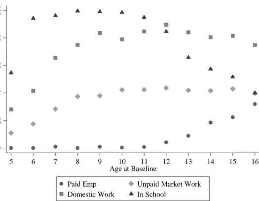
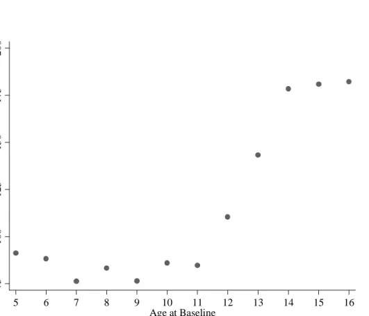
Paid work outside of the family’s home seems different from other types of work in the present context. First, participation in paid employment is not present in our baseline dataset until age 11 and exhibits a steep rise in incidence from age 13 on. Figure 1 pictures participation rates by age for paid employment, domestic work (chores, caretaking, etc), unpaid market work in the family farm or business, and school enrollment at baseline.Work in the family farm or business rises from ages 6 to 8. In contrast to paid employment, participation rates in the family farm or business and in domestic work stay roughly level from age 10 to 16. Second, paid employment appears more rigid in its hours than other work. This is evident in Figure 2 which plots the distribution of hours worked in the last week for the control sample at follow-up. At follow-up, the mode and median hours worked for a child under 17 in paid employment is 40 hours per week. The mean is 39.7 hours per week. Third, paid employment is less apt to be combined with
schooling than other types of work. One out of five children in paid employment enrolls in school. 61 percent of children working in the family farm or business enroll in school. Hence, paid
employment appears closer to the popular concept of child labor in our sample of poor families from the Ecuadorean highlands.
The interpretation of subsistence in the luxury axiom is central in the present discussion. Its definition within the luxury axiom is the standard of living at which the family feels it can afford to avoid child labor for an individual child. This is a perception of the household decision-maker.8 It will depend on how large the household is, the number and type of dependents in the household, and the net costs of alternative uses of a child’s time outside of child labor. That is, many of the factors that influence child time allocation through the budget constraint in a Becker (1965) style model can be incorporated into BV as heterogeneity in subsistence.
The incorporation of the child’s age into subsistence perceptions is especially important in the present application. The amount of money necessary to forego child labor increases with age.
8
Subsistence is treated as fixed and invariant across household attributes in the original model, because households are homogenous. The main result of the BV model, the characterization of child labor as a potential coordination failure, survives allowing for heterogeneity in subsistence levels (see Basu, Das, and Dutta 2009 for more discussion).
Food demands rise with age, especially around puberty. Schooling is an alternative to child labor, and the increase in schooling costs that comes with the end of primary school may influence how much money the family thinks it needs to avoid child labor. Figure 3 contains a plot of total school expenditures by age in the baseline data. Reported direct schooling costs (fees, books, uniforms, transport, meals, etc.) at baseline rise from $85 per child per year at age 11 to $180 by age 15.9 Rising schooling costs may be the simplest explanation for why families would feel that the amount of income necessary to avoid child labor would increase with age from age 11.10
C. The Luxury Axiom's Implications for the Impact of the BDH Transfer
With these two clarifications about the definition of child labor and the interpretation of
subsistence, the luxury axiom has clear implications for the impact of additional income on child labor. Changes in and affect child labor identically in the BV set-up. To focus on our discussion on the anticipated impact of the BDH on child labor, adult wages are fixed. Transfer income increases from 0 to . Potential child laborers are observed twice: before the transfer income is received and after receiving the transfer. The impact of an increase in transfer is heterogeneous depending on and .
A
w ti
ti
A
w si
The BV set-up implies that the BDH should reduce child labor if it allows families to afford to forego child labor. The transfer need not cover foregone child labor earnings in order to be effective. Because families that can cover their subsistence needs without child labor will choose to forego child labor earnings, the transfer can be associated with declines in family income in households where child labor declines.
The impact of the transfer should be largest for families with children that have yet to transfer from school to paid employment at baseline. We call these pre-transition children. Children in paid employment at baseline are revealed to be below subsistence at baseline.
9
9
The population of children in school at 15 is different than at age 11. An alternative measure of the rise in schooling costs associated with the end of primary school is to look at the average change in schooling costs for children that transition from primary to secondary between baseline and follow-up in the control sample. Average schooling costs per child rise from $126 per year to $193 per year for the 265 children in the control population that transition from primary school to secondary school between baseline and follow-up.
10
Higher child wages cannot explain higher child labor (directly) in the Basu and Van set-up. Child wages probably increase with age, but the only factors that enter the child’s labor supply decision are adult income, transfers, and the living standard necessary to afford no child labor. Child wages are an indirect schooling cost. Conceptually one can imagine that a given child’s wage enters the labor supply decision through subsistence perceptions as with direct schooling costs.
Subsistence increases with age. Given the small size of the transfer, it is unlikely that the transfer can offset the growth in subsistence needs that occurs with the child's aging between baseline and follow-up and compensate for the family's initial subsistence deficit. However, when children are above subsistence (not in paid employment) and in school at baseline, the transfer is more than the rise in schooling costs associated with aging. It is more likely that the transfer can protect the schooling status and delay entry into child labor for children that are in school and out of paid employment at baseline.
The impact of the transfer should be concentrated in families with few children.
Children require support, raising perceived subsistence needs. It is conceivable that the change in perceptions about subsistence will vary with the age of dependents. Very young children have little opportunity to contribute economically to the family but demand both consumption and time. Older dependents may have a different effect on subsistence perceptions. School age children are less time and more cash intensive. They also have the possibility of contributing economically. Hence, the model predicts less of an impact of transfer income when there are very young children present. The presence of other school age children mitigates the impact of the transfer if these children's economic contribution is less than their additional subsistence needs.
IV. MAIN FINDINGS
A. Empirical Methods
Our empirical strategy approach follows directly from the preceding section. Adult wages are determined by local labor markets. We treat the parish as the labor market and allow for urban-rural differences by including parish fixed effects λc. We control for the vector of baseline time allocation characteristics listed in table 1, E, as well as the other child and household level characteristics listed in the table. Age, household size, number of children 0-5, and number of school age children are recoded as dummy variables throughout the empirical work and denoted
a
λ . We present average treatment effects of the program, and consider heterogeneity based on the whether the child is pre-transition at baseline and the presence of other children at baseline.
Our reduced form results consider the impact of winning the lottery. We regress a child labor indicator on the controls above and an indicator for whether the child’s family won the BDH lottery:
11 l
1 0 0
icp c a i i r i ip
e = +α λ λ+ +βX +δE +γ +ε eq. (4)
where εipis an error term that is 0 in expectation conditional on the other controls listed in
equation (4). Standard errors are clustered at the parish level as that is the primary sampling unit. Imperfect compliance with the experiment creates a challenge in interpreting the reduced form. We use two-stage least squares to rescale the reduced forms and compute estimates of the BDH's impact. We replace in equation (4) with an indicator for whether the family receives the BDH as our measure of .We instrument for the non-random with . The lottery raises the probability of receiving the BDH by 31.9 percentage points. Hence, the two stage least squares results are simply a mechanical rescaling of the reduced forms, multiplying the reduced forms by 3.13. The assumption in interpreting this rescaling as the impact of the BDH for lottery winners is that winning the lottery does not itself influence child labor decisions beyond its effect on take-up. Heterogeneity in the effect of the transfer with pre-transition status or baseline household
composition is captured by interacting with the baseline characteristic i
l
i
t ti li
i
t Zi and instrumenting this
interaction with Zi*li. With the inclusion of parish fixed effects, our empirical approach only captures effects of the BDH that are net of any spillovers to the control population. Spillovers from the experiment are apt to be limited. Average parish population is 26,503, and there are on average 14 treated school age children participating in the experiment per parish.
B. Child labor declines with winning the lottery
Winning the BDH lottery is associated with a 2.2 percentage point decline in the probability a child 10+ at baseline works for pay at follow-up. IV results imply that BDH receipt is associated with a 7.0 percentage point decline in child labor. 17 percent of lottery losers work for pay at follow-up. Hence, the BDH is associated with a 41 percent reduction in child labor. These results are in table 2. The first column in table 2 contains the reduced form. The remaining columns instrument for BDH receipt with lottery assignment.
The decline in work for pay is driven by children who are in school and out of work at baseline ("pre-transition" children) continuing to not enter child labor. The decline in child labor in the pre-transition population is apparent in column 3 of table 2. There is a negligible effect of the BDH on work for pay in the population that is out of school or in paid employment at baseline. For the pre-transition population, the BDH is associated with a 12 percentage point decline in
12 child labor. The impact of the lottery is largest among the poorest of the pre-transition population. This is evident in Figure 4, which plots estimates of the impact of winning the lottery by per capita expenditure.
The pictured curve is the change in participation rates in wage employment at follow-up (lottery winners – lottery losers) by baseline per capita expenditures. It is computed by creating a grid of the baseline per capita expenditure distribution. For each point on the grid, the participation rates in paid employment are calculated separately for the treatment and control populations using local linear regression. The difference in participation rates in paid employment at follow up between the treatment and control populations is pictured for each grid point as is the 90 percent confidence interval. The X-axis is on a log scale. The sample is restricted to children 10 and older, in school, and not in paid employment at baseline. An obvious concern with comparisons of this type is whether the randomization remains valid at such a fine partitioning of the data. Figure 5 plots the probability a child's household wins the lottery by baseline per capita expenditures. The probability a household is treated appears balanced throughout the baseline per capita expenditure distribution.
Child labor declines for children in households with baseline per capita expenditures below $1414 per person per year. This is 98.5 percent of the sample. The declines in child labor are only statistically significant for baseline per capita expenditures below 348 per person per year. This is 32.5 percent of the sample (479 children in the restricted subset of pre-transition children).
Dividing the sample by baseline per capita expenditures significantly limits the number of observations, but there is still sufficient mass for analysis.
The baseline standard of living is only one part of the luxury axiom calculation. Household perceptions of subsistence also matter. The presence of other children makes the income necessary to cover basic needs greater. The data seem to bear this out: young children or multiple school age children eliminate the impact of the transfer. This finding is in columns 4 – 5 of table 2. Child labor declines with the BDH, but only when there is one school age child present. The magnitude of the decline in column 4 is such that the transfer eliminates child labor in families with only one school age child present (among lottery losers, 30 percent of children in households with only one school-aged child at baseline are child laborers at follow-up). One child under 5 also eliminates
13
the impact of the transfer (column 5).11 The presence of young children and additional school age children are correlated. Column 6 of table 2 allows the impact of the transfer to vary with the presence of other school age children, young children, and both. It is clear in these final columns that additional school age children essentially eliminate the impact the BDH, and young children attenuate the impact of the transfer.
The BDH affects large declines in child labor. However, these declines are all similar to what one would expect based on the association between child labor and expenditures we observe in the control population and the amount of the transfer. See appendix two for additional
discussion.
C. Declines in child labor are associated with fewer hours worked, increases in school enrollment, and reductions in total expenditures
In order to better understand and interpret the decline in child labor documented in the previous section, we consider the impact of the lottery on time allocation and expenditure patterns. We mimic the specifications of columns 3 and 6 in table 2.
There is no universally accepted definition of child labor (Edmonds 2007). The focus on paid employment seems appropriate in the present context, but it is possible that the income induces a shifting of labor to different types of work. We look at this directly in table 3. An alternative definition of child labor is market work (the combination of unpaid market work and paid employment). Columns 1 and 2 show that unpaid market work declines with the transfer. Since both paid employment and unpaid market work decline for the pre-transition population, market work overall declines. For the pre-transition population, the declines in unpaid market work are larger than the declines in paid employment. This result stems in part from the fact that participation rates are much higher in unpaid market work than they are in paid employment. For children who are the only school age child in the household at baseline, with no other young children present, the BDH appears to result in an increase in unpaid market work. That is, there is a hint of substitution from paid employment to unpaid market work with the transfer for children in families without other children present.
11
The impact of the transfer does not appear to vary with household size overall once one allows for heterogeneity in the number of school age children present at baseline. The oldest resident child at baseline generally experiences a larger treatment effect although the oldest child distinction is never statistically significant.
14
There is stronger evidence of shifting labor supply towards domestic work such as cooking, caretaking, and cleaning for the population whose paid employment is affected by the transfer. This evidence is in columns 3 and 4 of table 3. The rise in participation in domestic work is slightly smaller than the fall in paid employment documented in table 2. For pre-transition children, the transfer reduces paid employment by 12 percentage points. The rise in domestic work participation for this group is 8 percentage points. These magnitudes are consistent with two-thirds of the affected pre-transition children participating in domestic work instead of child labor. A smaller share of children shifts to domestic work in the population without other school age children present. The results in column 4 of table 3 (combined with column 6 table 2) imply that 40 percent of the decline in child labor is associated with increased participation in domestic work in the population without other children present.
This rise in participation in domestic work is associated with more hours in domestic work (not shown), but the change in paid employment is the dominant influence on the total hours worked by the child. The relevant results are in columns 5 and 6 of table 3. For pre-transition children, the decline in total hours is slightly less than would be predicted by the fall in paid employment. Average hours worked in paid employment is 40 hours per week. A 12 percentage point decline in participation should appear as 4.8 fewer hours worked per week. Column 5 of table 3 documents that pre-transition children work 3.65 fewer hours per week with the transfer. In the population without other children present, the decline in paid employment implies 15.5 fewer hours worked per week, but the column 6 results suggest 9.2 fewer hours. The rise in time in domestic work appears to absorb 41 percent of the decline in hours worked in paid employment for children with no other children present in the household (column 6).
School enrollment also increases with the BDH.12 The changes in school enrollment are similar in the population that avoids child labor and the population whose child labor status is unaffected. This is apparent in columns 7 and 8 of table 3. The schooling impact of the BDH does not seem to vary with whether the child is pre-transition. The schooling impact is slightly larger when there are no other children present, but overall, in schooling, we do not see the strong differences in the impact of the BDH that was evident for child labor. Taken together, we see less child labor, a bit more domestic work, but fewer total hours and more schooling with the BDH.
12
This result is also in Schady and Araujo (2008). Our estimated changes in schooling are slightly larger than that study, because we restrict our sample to an older (10+ at baseline) population where schooling is more elastic.
15 A corollary of the luxury axiom is that total expenditures can decline with a fall in child labor because of foregone child income. This theoretical result stems from the assumption that child labor is discrete. The discrete nature of time in paid employment in Ecuador has been documented above, and we observe declines in total expenditures in the populations with declines in child labor. Median wages in paid employment in the control sample at follow-up are $80 per child per month (for participants only). The interquartile range of wages is 40. Mean wages are $90, and the 95 percent confident interval ranges from $75 to $105 per employed child per month. With a transfer of $15 per month, the net effect of the decline in child labor plus the transfer is plausibly a decline in total expenditures.
Table 4 documents the declines in expenditures associated with the BDH. The observed declines in total expenditure are consistent with the fall in child labor. For pre-transition children, we observe a decline of $2.3 dollars per month in total household expenditures. The BDH is associated with a 12 percentage point decline in child labor per child. There are 1.8 pre-transition children per household in households with a pre-transition child at baseline. At the median wage, the change in child labor implies that the family is giving up $17.28 per month in child labor income. The BDH transfer is $15. Hence, net income declines by $2.28 with the BDH. For children living without any other children present, the decline in child labor of 39.5 percentage points implies $31.6 in foregone household income at median wages. With the transfer of $15 per month, the implied decline in net income is $16.6. We observe a decline of $13.6 in column 2 of table 4. The observed changes in consumption are extremely imprecise. This $3 difference is 6 percent of the standard error on the change in consumption for the population with no other children present. Nevertheless, the declines in expenditures are consistent with the decline in child labor for the affected population.
These expenditure findings are a validity check on the child labor results and the luxury axiom. It is plausible that some of the decline in expenditures is attributable to declines in child labor, rather than to the foregone income. For example, within the food category, we observe a decline in meals taken away from home (results not shown). However, the largest declines in expenditures in table 4 are in non-food items. Within non-food item categories, many of the largest declines in non-food expenditures are in low frequency purchase items. For pre-transition children, we see large (and statistically significant) declines in expenditures on TVs, stereos, and other appliances. For children without other children present, we see large and statistically
16 significant declines in furniture and bathroom appliances like hair dryers / shavers, etc. Thus, there is some evidence within categories of expenditures that the declines in expenditures are not driven by changes in the location where children spend their time.
D. Declines in child labor are not explained by a misunderstanding about possible conditions attached to the BDH transfer
The extent to which the impact of the transfer on child labor conforms to the predictions of the luxury axiom is striking. However, it is important to remember that the BDH experiment was conducted at a time when the government of Ecuador was promoting human capital with its rhetoric and emphasizing the importance of the BDH towards that goal. 25 percent of our sample (split evenly between treatment and control) think that BDH recipients are supposed to attend school. Schady and Araujo (2008) point out that, within the treated population, the increases in schooling over time are largest for those who erroneously believe that they are supposed to attend school to receive the BDH. Could mistaken beliefs about conditionality drive the child labor findings we report?
Three pieces of evidence are inconsistent with the hypothesis that mistaken beliefs about conditionality drive our child labor findings. First, the transfer is less than child labor earnings. Children in paid employment earn $80 per month per working child. The BDH transfer is $15 per household per month. If households thought that the transfer required schooling and that this meant no child labor, families would be better off simply turning down the transfer.
Second, all individuals are exposed to the social marketing, but the declines in child labor are concentrated in the subpopulation where the Basu and Van model predicts they should be: poor families whose children have not yet transitioned out of school and who have only one school age child present.
Third, our results do not vary substantively with these beliefs about the schooling requirements of the transfer. Beliefs about schooling requirements are not random, but we examine whether the impact of the BDH on child labor varies with these beliefs (measured at follow-up) in table 5. The declines in work for pay, total hours, and total expenditures are slightly larger in households that report believing that the transfer requires schooling. The differences are never statistically significant, and are not substantive in magnitude. The only margin where reported beliefs about schooling requirements substantively change the estimated effects of the
17 BDH is in school enrollment. Of course, as Schady and Araujo (2008) emphasize, this is also the place where interpretation is most difficult since children attending school answer that they are supposed to attend school with the BDH. We conclude from these various pieces of evidence that the impact of the BDH on child labor is unlikely to be explained by mistaken beliefs about possible conditions attached to transfers.
V. CONCLUSION
This study considers child labor responses to a lottery in Ecuador where families were randomly awarded the opportunity to receive $15 per month through the Bono de Desarrollo Humano program. We observe a surprising pattern of responses that match the predictions of the luxury axiom in Basu and Van (1998). The luxury axiom states that families make the child labor decision by asking whether they can afford to forego child labor. The child labor decision is intertwined with a family’s attempt to cover their subsistence needs. Our four main results are all consistent with the implications of the luxury axiom.
First, the luxury axiom implies that child labor can decline with an increase in exogenous (non-child labor) income, even if the increase in income does not cover foregone child labor earnings. The exogenous increase in income allows families to meet their subsistence needs without child labor's contribution. In the present case, we observe a 40 percent decline in child labor even though the BDH is less than 20 percent of foregone earnings.
Second, the luxury axiom implies that the impact of the BDH should be concentrated in children who have not yet made the school to work transition. Subsistence needs increase with the child's age because of rising food demands and rising costs of alternatives to child labor such as schooling. The BDH is less apt to put families above subsistence if they start off below
subsistence and the child ages in the year and a half between baseline and follow-up. The
documented declines in child labor are entirely among pre-transition children who have not yet left school for formal employment at baseline. Children already in paid employment at baseline are not affected by the transfer. Thus, the interpretation of our findings is that the transfer delays the age at which a child transitions to paid employment.
The transfer is also associated with a rise in school enrollment. The luxury axiom does not have any explicit prediction about schooling, but the rise in schooling may be useful for
18 Between one third and two thirds of the transfer is spent on schooling for children experiencing declines in child labor. Schooling costs are large and tend to be concentrated in certain times of the year. The transfer is larger than the rise of direct schooling costs that come with the start of
secondary school. Perhaps the transfer has such a large impact on child labor and schooling despite not covering foregone earnings because the transfer allows the household to afford the direct cost of schooling. This raises the question of why the child would not work a few hours, earn enough to cover schooling costs, and attend school. Hours worked in paid employment are concentrated around 40 hours per child per week. If this lumpiness of hours worked reflects some inflexibility in formal employment, then our results imply that the transfer allows the family to cover the cost of whatever factor was driving the child to work. It is not necessary that the transfer cover all of foregone earnings. If this characterization is accurate, the impact of transfers like those we study in this paper on child labor may be minimal if child labor hours were more flexible, allowing children to both work for pay and attend school. The importance of inflexible work hours in explaining why child labor seems to trade off with schooling has been mentioned frequently in policy discussions (see for example the Public Report on Basic Education in India 1999).
Third, the luxury axiom implies that the impact of the BDH should be larger for children in families with few other children present. With more dependents, the transfer is less likely to cover what the family perceives as its subsistence needs. We find no impact of the transfer on child labor when there is more than one school age child present at baseline, or when there are children under 5. Interestingly, despite the absence of BDH program effects on child labor, the impact of the transfer on school enrollment is sizeable and significant when there are other dependents present.
Fourth, the luxury axiom implies that increases in income can lead to declines in
expenditures because of foregone income from child labor. This implication is driven by the fact that child labor is discrete in the model and apparently close to discrete in our data. We observe declines in total expenditures that are similar in magnitude to foregone child labor earnings. We do not know whether families perceived the transfers as permanent or temporary. Hence, it is difficult to infer anything about whether families treat the transfers as permanent or transitory income changes.
The child labor findings we observe in our data do not seem to be driven by mistaken perceptions of BDH program requirements, but it seems reasonable to suppose that the social context influences our findings. In particular, the government’s social marketing campaign may
19 have been important. One way to internalize this context into the analytical framework of the Basu and Van model is to suppose that social marketing changes a household’s perceptions of
subsistence, or the perceived returns on educational investments. Social marketing might also influence the control population, the attitudes of bureaucrats and educators, or social norms more broadly. Hence, it is important to remember that our findings reflect the impact of a poverty alleviation program delivered in the context of a social marketing campaign. The relative
importance to our results of the social marketing campaign, the apparent indivisibility of hours in paid employment, the rise in school costs associated with the transition to secondary school, and the size of the cash transfer are unresolved issues in the current study.
The study's two main findings are that the response of families to the BDH experiment matches the predictions of the luxury axiom, and that child labor can decline even without
covering foregone earnings. These two findings highlight the central role poverty plays in the child labor decision, and illustrate the possibility of affecting large changes in child labor with relatively modest investments in poverty relief. Other studies have suggested the possibility of intergenerational poverty traps working through child labor itself (Emerson and Portela 2003), its impact on education (Barham et al. 1995), or child labor's influence on occupational choice (Banerjee and Newman 1993). It is difficult to predict the magnitude of the resulting multiplier effects from child labor reductions, but taken together these studies and our results raise the prospect of large returns to anti-poverty efforts.
REFERENCES
Attanasio, O., E. Fitzsimons, A. Gómez, D. López, C. Meghir, and A. Mesnard (2006), “Child education and work choices in the presence of a conditional cash transfer programme in rural Colombia.” IFS Working Paper, W06/01. London: Institute for Fiscal Studies.
Baland, J. and J. A. Robinson (2000), “Is child labor inefficient?”, Journal of Political Economy
108: 663-679.
Banerjee, A. and A. Newman (1993). "Occupational Choice and the Process of Development."
Journal of Political Economy, 101, 274-298
Barham, V., R. Boadway, M. Marchand, and P. Pestieau (1995). "Education and the Poverty Trap," European Economic Review 39 (7), 1257–75.
Basu, K. (2006), "Gender and Say: a model of household behavior with endogenously determined balance of power," Economic Journal, 116: 558-580.
20 Basu, K., and P. Van (1998), “The economics of child labor”, American Economic Review, 88: 412-427.
Basu, K., S. Das, and B. Dutta (2009), "Child labor and household wealth: Theory and empirical evidence of an inverted-U," Journal of Development Economics, forthcoming.
Becker, G. (1965), "A theory of the allocation of time", Economic Journal 75: 493-517. Cigno, A. and F. Rosati (2005), The economics of child labour, (Oxford University Press, Cambridge).
Doepke, M., and F. Zilibotti (2005), “The macroeconomics of child labor regulation”, American Economic Review 95: 1492-1524.
Doran, K. (2006), "Can we ban child labor without harming household welfare? An answer from schooling experiments," Unpublished paper (Princeton University, Princeton, NJ).
Edmonds, E. (2005), “Does child labor decline with improving economic status?”, Journal of Human Resources 40: 77-99.
Edmonds, E. (2006), "Child labor and schooling responses to anticipated income in South Africa,"
Journal of Development Economics 81(2): 386-414.
Edmonds, E. (2007), "Child Labor," in T.P. Schultz and J. Strauss, eds., Handbook of Development Economics, (Elsevier Science, Amsterdam, North-Holland) 3607-3710. Emerson, P. and A. Portela Souza (2003), "Is there a child labor trap? Intergenerational persistence of child labor in Brazil", Economic Development and Cultural Change
Fafchamps, M. and J. Wahba (2006), “Child labor, urban proximity, and household composition”,
Journal of Development Economics 79: 374-397.
Fan, J. and I. Gijbels (1995), Local Polynomial Modelling and Its Applications. New York: Chapman & Hall.
Filmer, D., and N. Schady (2008), “Getting girls into school: evidence from a scholarship program in Cambodia”, Economic Development and Cultural Change 56(3): 581-617.
Kruger, D. (2007), “Coffee production effects on child labor and schooling in rural Brazil”,
Journal of Development Economics 82: 448-463.
Levison, D., R. Anker, S. Ashraf, and S. Barge (1998), “Is child labor really necessary in India’s carpet industry,” in: R. Anker, S. Barge, S. Rajagopal, and M.P. Joseph, eds., Economics of Child Labor in Hazardous Industries of India, (Hindustan Publishing, New Delhi, India) pp. 95-133. Manacorda , M. (2006), “Child labor and the labor supply of other household members: Evidence from 1920 America”, American Economic Review 96: 1788-1800.
21 Manacorda, M., and F. Rosati (2007), "Local labor demand and child labor", Working Paper (Understanding Children's Work Project, Rome).
Paxson, C., and N. Schady (2009), “Does money matter? The effects of cash transfers on child development in rural Ecuador”, Economic Development and Cultural Change, forthcoming. The Probe Team (1999), Public Report on Basic Education in India (Oxford University Press, New Delhi, India).
Ravallion, M., and Q. Wodon (2000), “Does child labour displace schooling? Evidence on behavioural responses to an enrollment subsidy”, The Economic Journal 110(462):158-175 Rosenzweig, M., and R. Evenson, (1977), “Fertility, schooling, and the economic contribution of children in the rural India: An econometric analysis”, Econometrica 45: 1065 – 1079.
Schady, N. (2004), "Do macroeconomic crisis always slow human capital accumulation?", World Bank Economic Review 18: 131-154.
Schady, N., and M. C. Araujo (2008), "Cash transfers, conditions, and school enrollment in Ecuador", Economía 8(2): 43-70.
Schady, N., and J. Rosero (2008), “Are cash transfers made to women spent like other sources of income?”, Economics Letters 101(3): 246-48.
Schultz, T. P (2004), “School subsidies for the poor: evaluating the Mexican Progresa poverty program”, Journal of Development Economics 74(1): 199-250.
APPENDIX ONE: BACKGROUND ON THE BONO DE DESARROLLO HUMANO EVALUATION
Ecuador has three geographic areas—coast, highlands, and jungle. Administratively, the country is divided into provinces, cantons, and parishes. In 2005, there were 22 provinces, 219 cantons, and 874 parishes. Provinces span both urban and rural areas; cantons can be either entirely urban (as would be the case, for example, with the capital city, Quito), or a mix of urban and rural. Parishes are entirely rural or urban. In rural areas, parishes correspond roughly to villages; in urban areas, parishes frequently correspond to neighborhoods within a larger city. Of the 874 parishes in the country in 2005, 219 were urban, and 655 rural.
The parishes in the BDH evaluation were drawn from four provinces in the highlands region of the country: Carchi, Cotopaxi, Imbabura, and Tungurahua. Appendix Table 1.1
22 compares the sample of rural parishes included in the BDH evaluation to other rural parishes in Ecuador.
Appendix Table 1.1: Comparison of rural parishes in evaluation sample with other rural parishes
BDH evaluation sample (36 parishes)
Other parishes (779 parishes) Fraction of households in parish with:
electricity 0.889 0.719
telephone 0.116 0.087
connection to sewage system 0.265 0.160
garbage collection 0.183 0.148
that own a house 0.808 0.810
Source: 2001 Population Census
Households in the evaluation parishes appear to be somewhat better off than those in other rural parishes. For example, 89 percent of households in the evaluation rural parishes have access to electricity, compared to 72 percent for households in other rural parishes; and 27 percent of households in the evaluation rural parishes are connected to the public sewage system, compared to 16 percent in other rural parishes.
The INEC, the Ecuadorean national statistical institute, does not disaggregate data for urban parishes within the same canton—rather, it only provides averages for the entire canton. Appendix Table 1.2 compares the sample of urban cantons that were included in the BDH evaluation with other urban cantons in Ecuador, along a number of dimensions. As with the rural sample, urban cantons in our sample appear to be somewhat better-off than other cantons. For example, 92 percent of households in the evaluation urban cantons have access to electricity, compared to 84 percent for households in other urban cantons; and 52 percent of households in the evaluation urban cantons are connected to the public sewage system, compared to 39 percent in other urban cantons
23
Appendix Table 1.2: Comparison of urban cantons in evaluation sample with other urban cantons
BDH evaluation sample (25 cantons)
Other cantons(214 cantons) Fraction of households in parish with:
electricity 0.915 0.844
telephone 0.272 0.221
connection to sewage system 0.515 0.389
garbage collection 0.499 0.499
that own a house 0.708 0.710
Source: 2001 Population Census
Of course, households in the evaluation sample will be considerably poorer than the
averages for their parishes given that they are drawn from the poorest two fifths of the population. The first cash transfer program in Ecuador, the Bono Solidario, was launched in 1998, in the midst of an economic crisis. Bono Solidario made monthly transfers of US $15 to households, with no strings attached. Many of the households that received transfers were poor, but others were not— there were no clear rules for eligibility into the program. To ensure that transfers were better directed at poor households, the Government of Ecuador began a reform of the Bono Solidario
program in 2003 that would begat the BDH. To this effect, it developed the Selben index, a composite measure of household assets and access to social services. This was done as follows. First, a nationally representative household survey, the Encuesta de Condiciones de Vida (ECV), was used to select variables that were highly correlated with per capita expenditures, were easy to collect in the field by minimally trained enumerators, and were judged to be difficult for
households to manipulate—at least in the short run.
The exact set of variables included in the Selben was as follows: material of floor; type of lighting in household; availability of a shower; availability of a flush toilet; main source of fuel for cooking; whether a household owned land; number of household members per room in house;
24 number of children below 6 years of age; main language spoken by head of household; number of years of schooling of head of household and his spouse; whether or not the household was covered by a public medical insurance plan; whether or not the head of household had received loans from a bank in the last year; whether or not the household had an automobile, computer, color TV, telephone, washing machine, microwave, video machine, fridge, stereo, or oven (separate questions, given separate weights); whether or not there were handicapped members in the household; whether or not school-aged children were enrolled in school and, if so, whether the school establishment was public or private. Household income was not included in the calculation of the index, as it is very difficult to collect, in particular in rural areas. These variables were aggregated into a summary index by principal components. The cutoff for eligibility was then set at the 40th percentile of the index, again using the ECV.
Second, the Government launched a large-scale effort to collect information from
households on the variables that made up the Selben index. All households in rural areas, as well as households in selected urban areas with a high incidence of poverty could ask that the Selben survey be applied to them. On the basis of this survey, each household received a Selben score. Households with scores below the cutoff were then made eligible for cash transfers, while those with scores above the cutoff were made ineligible. (This process of constructing a so-called proxy means test is similar to that used by many other cash transfer programs in Latin America,
including PROGRESA in Mexico and Familias en Acción in Colombia.) As a result, a large number of households started receiving transfers for the first time, and transfers were gradually phased out for a large number of households that had previously received them. The name of the program was also changed from Bono Solidario to Bono de Desarrollo Humano.
The sample frame for the evaluation was limited to households who had recently become eligible for BDH transfers for the first time; BDH administrative data, which incorporated data on the Selben index, was used for this purpose. The sample was further limited to households who had at least one school-aged child at the time the Selben survey was collected. The original design of the evaluation was meant to be a regression-discontinuity study of the impact of the benefit amount. Thus, the sample was limited to households around the threshold of the first and second Selben quintiles. The logic behind this decision was that households in the first and second Selben quintiles were initially meant to receive transfers of different magnitudes, and the evaluation was meant to focus on the impact of “large” versus “small” transfers.
25 Appendix Table 1.3 compares the BDH evaluation sample with those in the nationally representative 2005/06 Encuesta de Condiciones de Vida (ECV).
Appendix Table 1.3: A comparison of households in the BDH evaluation sample and the 2005/06 ECV
BDH sample 2005/06 ECV
Proportion of children in school (age 10-17) 0.700 0.823 Proportion of children in paid work (age
10-17)
0.122 0.112
Proportion of children in unpaid work (age 10-17)
0.423 0.207
Proportion of HH with flush toilet 0.281 0.466
Proportion of HH with piped water in home 0.238 0.472
Proportion of HH with dirt floor 0.444 0.076
Note: sample limited to households with at least one child age 10-17.
Despite the fact that the evaluation parishes are wealthier than average for Ecuador, study subjects appear poorer.
The government ultimately decided to make transfers of the same magnitude to all
households. At that point, the original evaluation design was obviously not useful; a decision was made jointly by BDH administrators and World Bank staff to switch from a regression
discontinuity strategy to one based on randomization. Because the baseline survey was already being collected, it was no longer possible to draw a new sample of households. Instead, all of the households that had originally been drawn were randomly assigned to treatment or control groups. The randomization was done by World Bank and BDH staff. Households in the sample were assigned a normally distributed random number with mean zero and standard deviation one. All households with values zero or higher were assigned to the treatment group.
The BDH program has no clear timeline for benefits. As in PROGRESA and other cash transfer schemes in much of Latin America, households can continue to receive transfers more or
26 less indefinitely. On the other hand, it was foreseen that households assigned to the control group by the lottery would be folded into the program two years after the collection of the baseline (after the follow-up survey). Lottery losers and families ineligible for the BDH because of their Selben score were not separately identified at the time of the evaluation.
The Selben index was updated in 2008-09 (the first update since the original roll-out); this involved the collection of new information from more than a million households. The extent to which households are more likely to misrepresent their characteristics now that they are better aware that the survey determines eligibility for BDH transfers is unknown, but may be a serious problem. The Government of Ecuador has announced that it will publish a new roster of BDH-eligible households in August 2009.
APPENDIX TWO: TAKE-UP
The experiment gives lottery winners (the treatment group) the ability to apply for the BDH at local administrative offices. Lottery losers (the control group) are not supposed to receive the BDH. 39 percent of the control group receives the BDH. 31 percent of the treated group do not take-up the BDH.
Appendix Table 2.1 tabulates the descriptive characteristics from table 1 by lottery and take-up status. Columns 1 - 3 refer to lottery winners. Columns 4-6 summarize the attributes of lottery losers. For each group, the first two columns are summary statistics for those who receive the BDH and those that do not (respectively. The third column in each group contains regression coefficients from the regression of an indicator for BDH receipt on the listed baseline
characteristics and including parish fixed effects. Standard errors are robust and clustered at the parish level.
Appendix Table 2.1: Determinants of Take-Up by Treatment Status Children 10 and older at baseline
Lottery Status: Lottery Winners Lottery Losers
BDH Recipient Status: Recipient Non
DV:
Take-up Recipient Non
DV: Take-up
27
mean/se mean/se b/se mean/se mean/se b/se
Sample Size 772 352 1,124 399 630 1,029
Time Allocation
Paid Employment 0.11 0.14 0.00 0.10 0.14 -0.05
(0.01) (0.02) (0.06) (0.01) (0.01) (0.08)
Unpaid Market Work 0.45 0.37 0.04 0.38 0.44 0.04
(0.02) (0.03) (0.06) (0.02) (0.02) (0.07)
Domestic Work 0.83 0.81 0.06 0.81 0.84 -0.12**
(0.01) (0.02) (0.07) (0.02) (0.01) (0.06)
Total Hours, Market Work 9.18 10.13 0.00 7.80 9.42 0.00
(0.52) (0.88) (0.00) (0.64) (0.60) (0.00)
Total Hours, Domestic Work 8.66 10.06 0.00 8.74 8.18 0.00
(0.29) (0.59) (0.00) (0.42) (0.31) (0.00)
School Enrollment 0.72 0.64 0.10 0.75 0.68 -0.02
(0.02) (0.03) (0.14) (0.02) (0.02) (0.15)
Out of School or in Paid Employment 0.30 0.38 0.03 0.27 0.34 -0.07
(0.02) (0.03) (0.14) (0.02) (0.02) (0.15)
Individual Characteristics
Age (at baseline) 13.01 13.06 0.01 12.90 13.03 0.00
(0.07) (0.10) (0.01) (0.09) (0.07) (0.01)
Male 0.47 0.47 0.02 0.52 0.52 0.00
(0.02) (0.03) (0.05) (0.03) (0.02) (0.06)
Speaks Indigenous Language 0.09 0.14 -0.18* 0.09 0.08 -0.04
(0.01) (0.02) (0.09) (0.01) (0.01) (0.07)
Has Disability 0.01 0.01 0.01 0.02 0.01 0.23
(0.00) (0.01) (0.14) (0.01) (0.00) (0.16)
Oldest Resident Child 0.58 0.60 -0.01 0.56 0.61 -0.01
(0.02) (0.03) (0.03) (0.02) (0.02) (0.04)