University of Massachusetts Amherst University of Massachusetts Amherst
ScholarWorks@UMass Amherst
ScholarWorks@UMass Amherst
Doctoral Dissertations Dissertations and Theses
March 2015
Learning with Joint Inference and Latent Linguistic Structure in
Learning with Joint Inference and Latent Linguistic Structure in
Graphical Models
Graphical Models
Jason NaradUniversity of Massachusetts - Amherst
Follow this and additional works at: https://scholarworks.umass.edu/dissertations_2 Part of the Artificial Intelligence and Robotics Commons
Recommended Citation Recommended Citation
Narad, Jason, "Learning with Joint Inference and Latent Linguistic Structure in Graphical Models" (2015). Doctoral Dissertations. 316.
https://scholarworks.umass.edu/dissertations_2/316
This Open Access Dissertation is brought to you for free and open access by the Dissertations and Theses at ScholarWorks@UMass Amherst. It has been accepted for inclusion in Doctoral Dissertations by an authorized administrator of ScholarWorks@UMass Amherst. For more information, please contact
LEARNING WITH JOINT INFERENCE AND LATENT
LINGUISTIC STRUCTURE IN GRAPHICAL MODELS
A Dissertation Presented by
JASON NARAD
Submitted to the Graduate School of the
University of Massachusetts Amherst in partial fulfillment of the requirements for the degree of
DOCTOR OF PHILOSOPHY February 2015
c
Copyright by Jason Narad 2015 All Rights Reserved
LEARNING WITH JOINT INFERENCE AND LATENT
LINGUISTIC STRUCTURE IN GRAPHICAL MODELS
A Dissertation Presented by
JASON NARAD
Approved as to style and content by:
David A. Smith, Co-chair
Mark Johnson, Co-chair
Benjamin Marlin, Member
Andrew McCallum, Member
Joe Pater, Member
Kristina Toutanova, Member
Lori Clarke, Department Chair Computer Science
DEDICATION
For my parents,
Robert and Michelle
ABSTRACT
LEARNING WITH JOINT INFERENCE AND LATENT
LINGUISTIC STRUCTURE IN GRAPHICAL MODELS
FEBRUARY 2015
JASON NARAD
B.A., B.S., M.A., STATE UNIVERSITY OF NEW YORK AT OSWEGO M.S., STATE UNIVERSITY OF NEW YORK AT BUFFALO
M.Sc., UNIVERSITY OF EDINBURGH
Ph.D., UNIVERSITY OF MASSACHUSETTS AMHERST
Directed by: Professor David A. Smith and Professor Mark Johnson
A human listener, charged with the difficult task of mapping language to meaning, must infer a rich hierarchy of linguistic structures, beginning with an utterance and culminating in an understanding of what was spoken. Much in the same manner, developing complete natural language processing systems requires the processing of many different layers of linguistic information in order to solve complex tasks, like answering a query or translating a document.
Historically the community has largely adopted a “divide and conquer” strategy, choos-ing to split up such complex tasks into smaller fragments which can be tackled indepen-dently, with the hope that these smaller contributions will also yield benefits to NLP sys-tems as a whole. These individual components can be laid out in a pipeline and processed in
turn, one system’s output becoming input for the next. This approach poses two problems. First, errors propagate, and, much like the childhood game of “telephone”, combining sys-tems in this manner can lead to unintelligible outcomes. Second, each component task requires annotated training data to act as supervision for training the model. These anno-tations are often expensive and time-consuming to produce, may differ from each other in genre and style, and may not match the intended application.
In this dissertation we pursue novel extensions of joint inference techniques for natural language processing. We present a framework that offers a general method for constructing and performing inference using graphical model formulations of typical NLP problems. Models are composed using weighted Boolean logic constraints, inference is performed using belief propagation. The systems we develop are composed of two parts: one a rep-resentation of syntax, the other a desired end task (part-of-speech tagging, semantic role labeling, named entity recognition, or relation extraction). By modeling these problems jointly, both models are trained in a single, integrated process, with uncertainty propagated between them. This mitigates the accumulation of errors typical of pipelined approaches. We further advance previous methods for performing efficient inference on graphical model representations of combinatorial structure, like dependency syntax, extending it to various forms of phrase structure parsing.
Finding appropriate training data is a crucial problem for joint inference models. We observe that in many circumstances, the output of earlier components of the pipeline is often irrelevant – only the end task output is important. Yet we often have strong a priori assumptions regarding what this structure might look like: for phrase structure syntax the model should represent a valid tree, for dependency syntax it should represent a directed graph. We propose a novel marginalization-based training method in which the error signal from end task annotations is used to guide the induction of a constrained latent syntactic representation. This allows training in the absence of syntactic training data, where the latent syntactic structure is instead optimized to best support the end task predictions. We
find that across many NLP tasks this training method offers performance comparable to fully supervised training of each individual component, and in some instances improves upon it by learning latent structures which are more appropriate for the task.
TABLE OF CONTENTS
Page
ABSTRACT . . . .v
LIST OF TABLES. . . xiv
LIST OF FIGURES . . . .xv
CHAPTER 1. INTRODUCTION . . . 1
1.1 Overview . . . 4
1.1.1 Model Combination: Maintaining Uncertainty . . . 4
1.1.1.1 N-Best Pipelines . . . 7
1.1.1.2 Marginalization-based Decoding . . . 9
1.1.2 Marginalization-based Approaches to Training . . . 10
1.2 Joint Inference in Graphical Models . . . 13
1.2.1 Graphical Models . . . 13
1.2.2 Factor Graphs . . . 14
1.2.3 Inference . . . 16
1.3 A Comparison of Approaches to Joint NLP . . . 17
1.3.1 Joint Decoding . . . 17
1.3.1.1 Comparisons to Pipeline Decoding withn-best Lists . . . 17
1.3.1.2 Unidirectional vs. Bidirectional Information Flow . . . 18
1.3.1.3 Units of Exchange . . . 20
1.3.1.4 Other Approaches to Joint Decoding . . . 21
2. FACTOR GRAPHS, BELIEF PROPAGATION, AND COMBINATORIAL
CONSTRAINTS . . . .31
2.1 A Running Example . . . 32
2.2 Probabilistic Graphical Models . . . 34
2.2.1 Sequence Tagging with Probabilistic Models . . . 36
2.2.2 Factor Graphs and Log-Linear Models . . . 38
2.2.3 Factor Graph Sequence Models . . . 40
2.2.4 Log-linear Models . . . 41
2.3 Inference via Belief Propagation . . . 42
2.3.1 What Inference Accomplishes . . . 43
2.3.2 Belief Propagation with the Sum-Product Algorithm . . . 46
2.3.2.1 Computing Beliefs . . . 49
2.3.3 Loopy Belief Propagation . . . 49
2.3.4 Message Order . . . 51
2.3.5 Minimum Bayes-Risk . . . 52
2.4 Structured Models and Combinatorial Constraints . . . 54
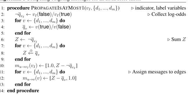
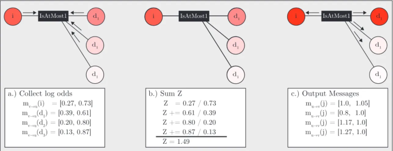
2.4.1 Message Computation for the IsAtMost1 . . . 55
2.4.2 Constraint Inventory . . . 59
2.4.2.1 Hard Factors . . . 61
2.4.2.2 Soft Factors . . . 63
2.4.2.3 Combinatorial Factors . . . 64
2.4.3 Constructing Joint Models . . . 65
2.4.3.1 Coordinating Between Tagging and Parsing Models . . . 67
2.5 Parameter Estimation . . . 69
2.5.1 Conditional Maximum Likelihood . . . 70
2.5.2 Optimizing with hidden variables . . . 71
2.5.3 Stochastic Gradient Descent . . . 72
2.5.4 Computing the Gradient . . . 74
2.5.5 Training with Latent Variables . . . 75
2.5.6 Learning to Coordinate Between Models . . . 77
2.5.7 Regularization . . . 78
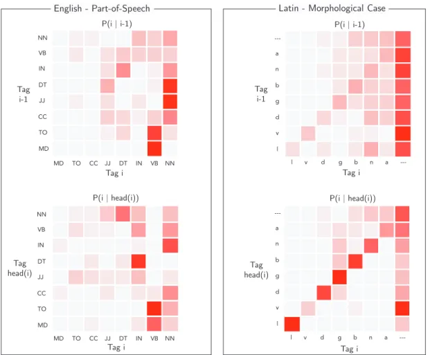
2.6.1 The Role of Syntax in Tagging . . . 80
2.6.2 A Joint Model of Tagging and Syntax . . . 82
2.6.3 Experimental Design and Results . . . 85
2.6.3.1 Data . . . 85
2.6.3.2 Model Configurations . . . 85
2.6.3.3 Design . . . 87
2.6.3.4 Results . . . 87
2.7 Conclusions . . . 88
3. FACTOR GRAPH REPRESENTATIONS OF SYNTAX . . . 91
3.1 Phrase Structure Parsing . . . 93
3.1.1 The Inside-Outside Algorithm . . . 98
3.1.2 Representing Phrase Structure in Factor Graphs . . . 105
3.1.2.1 Description of the CKY-TREEFactor . . . 109
3.1.2.2 Binarization . . . 117
3.1.2.3 Decoding . . . 119
3.1.2.4 Labeled Parsing in Factor Graphs . . . 120
3.1.2.5 Unary Chains . . . 123
3.1.2.6 Decoding . . . 124
3.1.2.7 Features . . . 125
3.1.2.8 Pruning . . . 127
3.1.3 Grammatical Rules as Factors . . . 129
3.1.3.1 Rule Representation . . . 129
3.1.3.2 Learning Rule Weights . . . 132
3.1.4 Experiments . . . 134 3.1.4.1 Data Sets . . . 135 3.1.4.2 Parsers . . . 135 3.1.4.3 Evaluation . . . 136 3.1.4.4 Unlabeled Parsing . . . 138 3.1.4.5 Label Parsing . . . 140 3.1.4.6 Grammar-based Parsing . . . 143 3.1.4.7 Decoding Speed . . . 144 3.2 Dependency Parsing . . . 148 3.2.1 Dependency Grammar . . . 148
3.3 Conclusions . . . 152
4. JOINTLY MODELING SYNTAX AND NAMED ENTITY RECOGNITION. . . .156
4.1 Overview of Named Entity Recognition . . . 158
4.1.1 The Relationship Between Syntax in NER . . . 160
4.2 Joint Modeling via Grammar Augmentation . . . 162
4.3 Description of Joint Model . . . 165
4.3.1 Modeling Named Entity Prediction . . . 166
4.3.1.1 A Combinatorial Factor for Semi-CRFs . . . 168
4.3.2 A Joint Model of NER and Constituent Syntax . . . 171
4.3.3 Features . . . 175
4.3.3.1 Features for NER factors . . . 175
4.3.3.2 Features for parse factors . . . 175
4.3.3.3 Features for coordinating factors . . . 176
4.4 Experiments . . . 176
4.4.1 Data . . . 176
4.4.2 Experimental Design . . . 177
4.4.3 Results . . . 179
4.4.3.1 The Case for Joint Inference . . . 179
4.4.3.2 A motivating example for Joint Inference . . . 183
4.4.3.3 The Effect of Joint Inference on Parsing Performance . . . 183
4.4.3.4 Advancing the State-of-the-Art . . . 185
4.5 Conclusions . . . 187
5. JOINT MODELS FOR RELATION EXTRACTION. . . .190
5.1 An Overview of Relation Extraction . . . 191
5.1.1 Factor Graph Models for Relation Extraction . . . 194
5.1.2 Factors for Coordinating Relation Extraction and Syntax . . . 195
5.2 Experiments . . . 197
5.2.2 Model Configurations . . . 199
5.2.3 Features . . . 201
5.2.4 Design . . . 203
5.2.5 Results . . . 204
5.2.5.1 Performance of Latent Syntactic Structure Models . . . 204
5.2.5.2 Dependency Structure vs. Phrase Structure . . . 206
5.3 Conclusion . . . 206
6. SEMANTIC ROLE LABELING WITH LATENT SYNTAX . . . .208
6.1 Semantic Role Labeling . . . 209
6.1.1 The Role of Syntax in SRL . . . 211
6.1.2 Related Work . . . 215
6.2 Factor Graph Models of SRL . . . 217
6.2.1 Baseline Model: SRL without syntax . . . 217
6.2.2 Joint Approaches to Sense and Role Prediction . . . 219
6.2.2.1 Modeling Valency with Accumulating Chains . . . 222
6.2.3 A Joint Model of Dependency Parsing and SRL . . . 224
6.3 Experiments . . . 226 6.3.1 Data . . . 226 6.3.2 Features . . . 226 6.3.3 Experimental Design . . . 230 6.3.4 Evaluation . . . 233 6.3.5 Results . . . 234 6.3.6 Valency Results . . . 237 6.3.7 Performance on SRL Frames . . . 238
6.3.7.1 An Analysis of Induced Syntactic Structure . . . 239
6.4 Conclusion . . . 247
7. CONCLUSION . . . .249
7.1 Future Directions . . . 254
7.1.1 Additional Latent Linguistic Structure . . . 254
7.1.1.2 Orthography and Phonology . . . 256 7.1.2 Exploring New End Tasks . . . 257 7.1.3 Incorporation of Approximate or Pruned Approaches to
Inference . . . 259 7.2 Final Thoughts . . . 261
LIST OF TABLES
Table Page
2.1 Tagging accuracy for English and Latin . . . 88
3.1 Features for span-factored constituent parsing . . . 126
3.2 OntoNotes data statistics . . . 135
3.3 Performance of the parsers in an unlabeled evaluation . . . 138
3.4 Label parsing performance . . . 141
3.5 NP prediction results . . . 143
4.1 NER and constituent syntax alignment statistics . . . 160
4.2 Features for NER factors . . . 174
4.3 Features for coordination factors . . . 175
4.4 F&M09 OntoNotes data statistics. . . 177
4.5 NER baseline and joint model performance on the OntoNotes corpus . . . 181
4.6 Standalone and joint parsing performance on the OntoNotes corpus . . . 185
5.1 Relation extraction results on ACE . . . 205
6.1 SRL Results on CoNLL 2009 data sets . . . 235
LIST OF FIGURES
Figure Page
1.1 Annotations for three common NLP tasks . . . 5
1.2 A pipeline approach to model combination . . . 6
1.3 Failure of the Viterbi approximation . . . 8
1.4 Bidirectional information flow via belief propagation . . . 19
2.1 Representations of graphical models . . . 39
2.2 A linear chain CRF represented as a factor graph . . . 41
2.3 BP message calculations: variable to factor . . . 47
2.4 BP message calculations: factor to variable . . . 48
2.5 A factorial CRF . . . 50
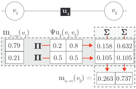
2.6 Outgoing message computation for the ISATMOST1 factor . . . 56
2.7 Message Computations for ISATMOST1 Factor . . . 58
2.8 Coordinating models with soft NANDfactors . . . 69
2.9 Heatmaps of conditional tag probabilities. . . 81
2.10 A joint model of tagging and parsing. . . 84
3.1 A phrase structure tree . . . 92
3.2 Inside&Outside trees. . . 102
3.3 Variables for phrase structure syntax . . . 108
3.5 Pseudocode of a right-branching binarization . . . 118
3.6 Binarized trees . . . 119
3.7 Pseudocode for unlabeled parser decoding . . . 121
3.8 Graphical depiction of the labeled parsing model . . . 122
3.9 Number of distinct span labels at varying span widths . . . 128
3.10 Grammatical rules as factors . . . 130
3.11 Pseudocode for rule factor learning with the Perceptron algorithm . . . 133
3.12 A comparison of parser decoding speeds . . . 146
3.13 A non-projective dependency tree . . . 150
4.1 A sentence annotated with syntax and NER . . . 159
4.2 Unaligned entities . . . 162
4.3 Grammar transformations for joint parsing and NER . . . 163
4.4 Semi-Markov models . . . 168
4.5 Pseudocode for the SEMI-CRF factor propagator . . . 170
4.6 A joint model of NER and phrase structure syntax . . . 172
4.7 An example of joint inference improving both syntax and NER analyses. . . 184
5.1 Relationships between syntax and relation extraction . . . 192
6.1 An example sentence with dependency tree and SRL annotations . . . 210
6.2 Correspondence between syntax and SRL predicate-argument pairs . . . 212
6.3 An example of crossing syntactic and SRL dependencies . . . 214
6.4 Modeling valency in SRL . . . 223
6.6 SRL frame arity across models . . . 238
6.7 Examining induced latent syntax for SRL . . . 240
6.8 English gloss for Japanese example in Fig. 6.7. . . 242
6.9 German NP structure . . . 245
CHAPTER 1
INTRODUCTION
When humans interpret language they infer a rich hierarchy of linguistic structures prior to constructing a semantic and pragmatic representation. Many of the tasks commonly ex-plored in natural language processing (NLP) are approached in the same way: first, the system recovers the relevant supporting linguistic structure (a parse tree, a tag sequence, etc.), which it then utilizes it to improve performance on the desired task. However, the working assumption underlying most NLP research is that linguistic processing can be modularized (often into lexical, morphological, syntactic, semantic, and pragmatic infor-mation), and that these modules can be modeled and trained independently. The resulting models can be composed in a serial fashion, feeding the output of one component forward to serve as input to the next, in a pipeline, in order to perform complex NLP tasks.
A typical pipeline might comprise a tagger, a parser, and anend task- the goal of the system. While the notion of an end task varies, we consider tasks like named entity recog-nition, relation extraction, and semantic role labeling to be sufficiently close to a user’s goal to be considered end tasks. Beginning with a sentence of raw text, a tagging model might pair each word with its most probable part-of-speech tag, before passing this information forward to the parser. The parser, leveraging the additional information provided by the tag sequence, assigns the most probable tree, and so forth. This provides a great deal of struc-tured information from which to make end task predictions, but each model pushes forward only a fraction of the information it captures, and information never flows backward.
pro-resolve ambiguity jointly (MacDonald, 1993; Plaut et al., 1996; Trueswell et al., 1994; Treiman et al., 2003). Similar strategies have been pursued in the NLP community (Poon and Domingos, 2007; Finkel and Manning, 2009; Lee et al., 2011; Singh et al., 2013a), yet so-calledjoint inferencetechniques have yet to become the standard approach to model composition. We hypothesize that this may be in part due to the lack of a flexible, gen-eral framework for constructing models for joint inference, with the ability to efficiently represent highly-structured models (such as models of syntactic structure). Additionally, we observe thatjointly annotated data– a single data set annotated for multiple tasks, suf-ficient for training all the models of a pipeline system – is scarce, and in most instances the outputs of intermediary models are never evaluated nor utilized other than to improve performance on a singular end task.
To this end we present a general approach for constructingjoint models: models which unite more than one task-specific model, which we refer to as a component model, and where information is shared freely between them during inference. Unlike the pipeline approach, information can flow in both directions. In theory this allows a joint model to recover from errors made by components which appear early in the pipeline, preventing further errors from accumulating downstream.
We argue that factor graphs (Kschischang et al., 2001) are an ideal formalism for defin-ing joint models. Factor graphs are a type of graphical model which are capable of repre-senting many common NLP models, and provide many characteristics which are beneficial for joint modeling in NLP:
• In a factor graph there exists a natural semantics for modeling dependent compo-nents, and this provides a principled method for connecting two component models, using probability theory as the language of coordination. Thus factor graphs provide a means of constructing joint models from common single-task models.
• In a joint model, dependencies between component models often create cyclic depen-dencies (loops). In a factor graph, there are inference algorithms (belief propagation,
Pearl (1988)) which provide approximate solutions for arbitrary graph structures, even those with cyclic dependencies. Therefore, factor graphs have a mechanism for reasoning with joint models.
• One of the most common components of an NLP pipeline is a parser, which produces a syntactic analysis for each sentence. Due to the combinatorial nature of syntactic structure, incorporating a model of syntax can lead to difficult, if not intractable, inference. Following the recent work of Smith and Eisner (2008), this problem can be circumvented in factor graphs through the use of specialized combinatorial factors.
Having addressed the problem of constructing and reasoning with joint models, we investigate new methods for training them. In order to train an NLP pipeline in the typical fully-supervised case, each component requires its own training data. For a joint model, the data requirements are significantly more demanding, as a single data set must be annotated with the labels for each task. Annotated data is already exceedingly scarce for most tasks in most languages, making this a very burdensome requirement.
To counter this we propose a paradigm shift away from the traditional motivation for joint inference, in which two or more tasks benefit mutually from fully-supervised joint training (Finkel and Manning, 2009), and focus instead on the scenario where joint infer-ence is applied solely towards improving performance of a single task. In this scenario, we can reduce the labeled data requirements of joint modeling by treating all supporting models (component models which are not the end task) as latent, or unobserved during training, requiring no training data of their own. For these models training supervision comes only indirectly, through the annotations of the end task, and is propagated through model dependencies during inference. In this scenario joint inference offers something new: a principled approach to learning with a combination of supervised and unsupervised components in a task-directed manner. We show, across a variety of NLP tasks, that this method provides performance comparable to fully-supervised training while requiring far
less training data, and in some circumstances even improving over identical models using gold or parser-produced annotations.
1.1
Overview
1.1.1 Model Combination: Maintaining Uncertainty
The natural language processing community works largely under the assumption that language can be effectively partitioned into largely independent modules – phonology, morphology, syntax, and semantics – each of which can be tackled independently. Each model assumes that all prerequisite steps have already been solved, and the input annotated accordingly. For example, a parser typically assumes the input has been part-of-speech tagged, and a semantic role labeling system typically assumes the input has been parsed.
But this strategy is only optimal when the tasks are largely independent of one another, i.e., that the solution to the latter problem does not influence the former. In the pipeline approach, errors made by earlier components force the following components to base their predictions on erroneous information, making it more likely for additional errors to accrue. If the models are dependent, information from later components could influence these early decisions. Methods ofjoint decodingaim to solve this problem. Starting from pre-trained models for individual tasks, joint decoding methods aim to find the optimal solution by considering information from all component models jointly. This may be the best solution for the entire pipeline (i.e., the bestglobalsolution), or it could be the optimal solution for only a subset of these components, conditioned on others.
In order to provide some context in which to discuss the problem of model combination, let us consider the task of semantic role labeling. Semantic role labeling (SRL) is the task of identifying basic semantic relationships in text. Given a sentence, the first step is to identify key verbs, known aspredicates, and group them with their associated arguments. Each argument is given a label to describe the nature of its relationship with the predicate, known as its semantic role (i.e., agent, patient, instrument, etc..) For the example sentence
a.) Part-of-speech Tags b.) Dependency Parse c.) Semantic Role Labels
The cat scratched the man DET NN VB DET NN
The cat scratched the man The cat scratched the man AGENT PATIENT
Figure 1.1. Annotations for three common NLP tasks.
“The cat scratched the man”, the correct SRL analysis identifiesscratched as a predicate,
cat andman as its arguments, and labels them AGENT and PATIENT respectively. These
annotations are shown in Fig.1.1c.
Current state-of-the-art SRL systems require a parsing component. In turn, because part-of-speech tags are required to train the parsing model (Fig.1.1a), the system will re-quire yet another model to tag words with their parts-of-speech. We can define a set of models that reflect this this hierarchy:
ModelT ags =P(T ags|W ords,ΘT ags)
ModelT ree =P(T ree|T ags, W ords,ΘT ree)
ModelSRL=P(SRL|T ree, T ags, W ords,ΘSRL)
(1.1)
whereModelT ags, ModelT ree, andModelSRLare models for part-of-speech tagging,
pars-ing, and SRL,T ags, T ree, and SRLare the predicted variables, ΘT ags,ΘT ree,ΘSRL are
the corresponding model parameters, andW ords is a variable representing a sequence of words provided to each model as input. During training a parameter estimation method is used to optimize each model’s parameters. In a supervised pipeline approach (Fig. 1.2) each model is trained independently, and requires its own annotated data set. During testing these models are utilized to annotate raw text with SRL annotations. Models for tagging, parsing and SRL will be defined in full detail in Chapters 2, 3 and 6, but for now let us consider how todecode(i.e., utilize the model’s predictions to assign structure to raw text) using these models on an arbitrary sentence.
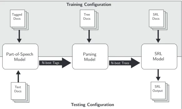
Tagged Docs Part-of-Speech Model Text Docs Tree Docs DocsSRL SRL Output SRL Model Parsing Model
N-best Tags N-best Trees
Testing Configuration Training Configuration
Figure 1.2. A pipeline approach to model combination. Individual models are trained in-dependently from their own task-specific annotations, i.e. tagged documents are annotated with part-of-speech tags, tree documents with syntactic trees, and SRL documents with predicate-argument pairs. These data sets may come from difference sources (top). During testing, where the goal is to use the system to make end task predictions for new data, the only input to the system is raw text. Each successive model applies an additional layer of annotation, propagating it forward to be used as input to the next (bottom). This is often the single most probable analysis, but components can also propagate forward larger lists of analyses (known as ann-best list, of sizen) in order to give later components some chance at recovering from a poor decision early in the pipeline.
Our goal is to find the most probableSRLanalysis, but, due to the hierarchical nature of the dependencies between these three models, finding this solution requires us to first consider the values of theT ree and T ags variables. However, in this scenarioT ree and
T agarelatent variables: we have models specifying distributions over these variables, but
their actual values are unknown. Here we present and contrast two approaches to dealing with these latent variables. The first decoding strategy truncates the latent variable distri-butions to a set of their most probable elements. A second decoding strategy relaxes this approximation, considering each possible analysis of latent structure and contributing its probability mass toward theSRLsolutions that are most compatible with it.
1.1.1.1 N-Best Pipelines
Perhaps the most straightforward approach to decoding a set of dependent models is to process each model in turn, taking the output from each model and using it as input to the next. Here the model dependencies impose a natural order, beginning with theT ag predic-tion, proceeding toT reeprediction, before finally reaching the goal,SRLprediction. This is aptly referred to as ann-best pipeline, where nis the number of analyses put forth by each component model (Figure 1.2). When the output from each model is its single best hypothesis,n= 1, this strategy can be summarized by the following equation:
GOAL1−best= arg max s∈S
P(SRL=s|T ree=t, T ags=p, W ords=w,ΘSRL)
max
t∈T P(T ree=t|T ags=p, W ords=w,ΘT rees) max
p∈P P(T ags=p|W ords=w,ΘT ags)
(1.2)
where S, T, and P are the sets of all possible SRL analyses, trees and tag sequences, respectively, and GOAL1−best is the best SRL analysis, conditioned on the
single-best tree and tag sequence.
This is a very practical approach, but when viewing this decoding strategy as a maxi-mization over each model in turn, it becomes clear that this is merely an approximation of a more exhaustive search. The approximation used here, known as the Viterbi approximation (in reference to the Viterbi decoding algorithm for hidden Markov models (Viterbi, 1967)), replaces each distribution with the most probable element of that distribution. This could also be viewed as three applicationsmaximum a posteriori(MAP) decoding, one for each of the three models, or as a case ofn-best decoding, wheren= 1.
While attractive from a practical perspective, pipeline approaches – both the Viterbi ap-proximation and the more generaln-best list decoding strategy – are severely handicapped when it comes to finding globally optimal solutions in NLP. In general, if the distribution of a preceding component is peaked (i.e., concentrated primarily on a small percentage of the analyses), the Viterbi approximation has a greater chance of selecting the correct
hy-The cat scratched the man DET NN VB DET NN
The cat scratched the man DET NN VB DET NN
The cat scratched the man DET NN VB DET NN
Syntax Analysis t1: P = 0.3 Syntax Analysis t2: P = 0.2 Syntax Analysis t3: P = 0.2
AGENT PATIENT AGENT PATIENT AGENT PATIENT
Figure 1.3. Failure of the Viterbi approximation. The top three trees of the parsing model’s distribution are shown, along with the correct SRL analysis below. SRL dependencies that are supported by the syntactic analysis are shaded in green, and those which do not are shaded in grey. The solution chosen by the viterbi approximation (leftmost tree) does not maximally support the correct SRL analysis (shown below each tree), as it shares only one of the SRL solution’s two arcs. In comparison, if the entireModelT ree distribution is
utilized the correct SRL analysis would receive additional (and greater) support from trees
t2 andt3.
pothesis. If the distribution is flatter, the model is less certain, the most probable analysis inherently a poorer approximation to the full distribution.
To understand how this affects model combination in practice, consider the example outlined in Figure 1.3. Here we depict three syntactic trees and their probabilities as spec-ified byModelT ree, paired with the correct SRL analysis. Let us assume that a syntax tree
provides evidence for an SRL analysis if there exists a corresponding syntactic dependency for each SRL dependency. When using the Viterbi approximation, ideally the most prob-able parse tree provides the maximum amount of evidence in support of the correct SRL analysis. However, here we find that the most probable parse tree,t1 with probability0.3,
is incorrect, and only partially supports the correct SRL analysis. The most probable SRL analysis under the distributionP(SRL|T ree = t1, T ags =p, W ords =w), conditioning
on incorrect information, is also likely to be incorrect.
In this case, broadening the the approximation to include all three parse trees would allow the model to include additional information from tree t2 andt3 that would be
bene-ficial to SRL prediction. However, in practice this strategy is flawed: the space of possible parse trees for a sentence is often too large to tractably pass forward from one component to
another. We now present an alternative method to decoding in which all syntactic analyses contribute in part to the decoding of the SRL model.
1.1.1.2 Marginalization-based Decoding
In a1-best decoding strategy only a model’s most probable analysis will affect the dis-tributions of later models. All other information about the model distribution is discarded at each step. An alternative approach, which we will refer to as marginalization-based decoding, generalizes over the n-best list approach, and provides a method for including more of the information captured by the latent distributions. It does this bymarginalizing
(summing over) all possible values for the latent variables (T reeandT ags):
GOALM arg= arg max s∈SRL
X
t∈T X
p∈P
P(SRL=s|T ree=t, T ags=p, W ords=w,ΘSRL)
P(T ree=t|T ags=p, W ords=w,ΘT rees)
P(T ags=p|W ords=w,ΘT ags)
(1.3)
whereGOALM arg is once again the single most probable SRL analysis, but this time
con-ditioning on all possible values of latent trees and tag sequences. This makes it more robust to the effects of flatter model distributions.
Returning to the example analyzing the effect of parser decoding on the SRL model (Fig. 1.3), recall that the Viterbi decoding strategy selects the most probable parse tree,t1,
and ModelSRL conditions upon it when finding the most probable SRL solution. Tree t1
provides only partial support for the SRL analysis, with one of the two correct SRL de-pendencies having a corresponding syntactic dependency. Using the marginalization-based decoding strategy, summing over trees will provide nearly half (P(t2|T ags=p, W ords= w) +P(t3|T ags = p, W ords = w) = 0.2 + 0.2 = 0.4) of the latent distribution’s
prob-ability mass to work in favor of the correct SRL solution. The sum of support for the correct analysis now outweighs the support for the incorrect analysis,0.4to0.3. For
illus-sands of possible trees for reasonably-sized sentences, and this mass must be distributed across many more trees, making the distribution inherently flatter and the Viterbi approach a poorer approximation of the full distribution.
We conclude with a clarification. The n-best and marginalization-based approach to decoding are useful for illustrating the difference between how model combination is typ-ically done in practice, as an approximation, and the more general marginalization-based approach. However, the models we propose are joint. Joint models unite the advantages discussed here (maintaining uncertainty at each step) with bidirectional information flow. This allows the beliefs of the later models to influence other models which would appear earlier in the pipeline. For instance, bidirectional information flow allows the beliefs of the SRL model to influence the parsing model, during both decoding and training. Instead of taking a set of pre-trained models as input to decoding, a joint model provides just one (individual component models are not factored out).
1.1.2 Marginalization-based Approaches to Training
We have presented an initial set of motivations for preferring a marginalization-based or joint decoding strategy over alternatives like n-best lists or Viterbi decoding. By operating on full distributions marginalization-based decoding avoids some of the potential pitfalls of approximate solutions to the global problem. But if this is our ideal decoding strategy, then what is the corresponding ideal method for training? Here we describe an analog to training we refer to as amarginalization-based training, which extends to optimization the philosophy of working with full distributions.
Let us start by discussing the pipeline approach to training. During training in this scenario, there are no latent variables. In the case of our SRL example, the SRL model is given the true values forSRL, T ree, and T ags. The Tree model would observe the true analyses forT ree andT ags, and so forth. These true analyses are derived not from the output of a previous model, as it is during testing, but are provided in annotated data. This
decoupling allows the models to be trained independently of each other, as illustrated in Fig. 1.2 (top). Optimizing the set of models can then be done as follows:
ΘM L−SRL = arg max ΘSRL n Y i=1 P(SRLi|T reei, T agi, W ordsi,ΘSRL)
ΘM L−T ree = arg max
ΘT ree n
Y
i=1
P(T reei|T agi, W ordsi,ΘT ree)
ΘM L−T ags = arg max
ΘT ags n
Y
i=1
P(T agsi|W ordsi,ΘT ags)
where i corresponds to the ith item from the training data. This type of optimization is known as maximum likelihood estimation (MLE). In MLE the goal is to optimize the likelihood of the parameters given the data, L(Θ|x). This is equivalent to maximizing
P(x|Θ), and thus the right hand side of each equation is a likelihood. Each instance of the training data is treated as independently generated, thus the likelihood of generating the entire data set is the product of all individual likelihoods.
There are some practical advantages to this approach. It is easier to find a separate data set for training each model than it is to find a single data set annotated for all three tasks, and it is also easier to train each model independently than to jointly optimize all models simultaneously. However, the disadvantage to training each model off an unrelated data set is that there will be some degree of domain or genre mismatch between them. Gildea (2001) shows that a parser trained on a corpus of newswire performs notably worse when tested on a mixed-domain data set. A similar problem exists when training systems off of several task-specific data sets. For instance, both the SRL and parsing models utilize parse trees during training, each from their own respective data sets. During decoding, the trees used by the SRL model are obtained from the parsing model. If these trees are not
representative of the trees the SRL model was trained on, the setting is identical to testing on out of domain data, and may be subject to similar performance loss.
In this thesis we propose a different strategy for training dependent models. Instead of training each model toward its own goal (i.e. a tagging model which attempts to best reproduce the gold tags from a corpus, a parsing model which attempts to reproduce the gold trees from another), we train all models toward one goal: improving performance on the end task. In the example case, the end task is SRL. Once we treat component models as parts of one larger, end-task directed model, there is no need to require task-specific annotations for each component model.
In theory this allows us to perform a complex end task like SRL, without requiring any training data for supporting tasks, like part-of-speech tagging or parsing. The resulting optimization on a joint model has the following form:
ΘM L−M arg = arg max ΘSRL,ΘT ree,ΘT ags Y i X t∈T,p∈P
P(SRLi, T reei =t, T agsi =p|W ordsi,ΘSRL,ΘT ree,ΘT ags)
(1.4)
whereSRLi is the correct SRL structure for theith training example, and we once again
sum over the latentT agandT reevariables. But this is during training – if supervision for these models is not required, what constitutes a probable tree or tag sequence? What these models will learn to represent is something more abstract, with supervision coming only indirectly, through the end task annotations. The fact that this is a joint model is what allows the error signal, originating with end task annotations, to propagate out and influence these latent structures. Simultaneously, we provide general constraints on the kinds of latent structures are permissible. For syntax, these constraints force the latent structure to be a directed graph or a tree. The learned latent structure will be one that optimizes Eq. ??
This discussion has provided a high level view of the approach pursued throughout this dissertation, leaving open the question of how we construct models, and how this method compares to other approaches. In the next section we introduce graphical models, a framework which we argue is convenient for constructing joint models, and performing joint inference.
1.2
Joint Inference in Graphical Models
We have previously described our marginalization-based approach to both model train-ing and decodtrain-ing. This goal requires information to be shared between component models, but we have not yet discussedhowthis communication is possible. The answer lies in in-ference, the process of drawing conclusions from data by using a statistical model. In this section we introduce graphical models, a powerful framework for representing and reason-ing with probabilistic models. Here inference will be used to answer the question, for a variable xand a valueq, “Given values for certain variables, what is the probability that
variable x has value q?”. The answer provides a key component, marginals, required for
training these models when using a gradient-based optimization method.
1.2.1 Graphical Models
Graphical models are a family of formalisms that use graph theory to express proba-bilistic relationships, namely conditional independence assumptions, which are useful for defining efficient inference algorithms. Here we provide a brief overview of graphical models, before discussing them at depth in Section 2.2 (pg. 34).
A probabilistic model encodes a problem domain using a set of random variables, the value of each variable capturing the state of particular aspect of the world. In NLP, a random variable may represent a word’s part-of-speech tag, a syntactic dependency between two words, or named entity over a span of words. A probabilistic model defines a distribution
over these variables, specifying the probability for any possible assignment of values to the variables in the model.
But a distribution over a set of nvariables, each withm values, yieldsO(mn)
config-urations, growing exponentially with the number of variables in the model. The models presented in this dissertation will often contain thousands, if not tens of thousands of vari-ables, and thus working with the distribution directly would be intractable.
Graphical models are a type of probabilistic model which use graph structure to rep-resent a factorization of this distribution. Variables correspond to nodes in the graph, and the graph’s edges encode dependencies between variables. More precisely, theabsenceof edges in the graph specifies the conditional independence properties of the model (this is described in detail in Section 2.2 on pg. 34). This allows graphical models to factor the dis-tribution as the product of many simpler functions, each of which deals with a much smaller subset of variables. The sparser the connections are in the graph, the more compactly the distribution can be represented using a graphical model.
This is the key to tractable representations of probabilistic models, but it is also a con-venient factorization: a sparsely connected graph provides a more compact representation of the distribution which helps to support efficient inference, but it simultaneously com-plements the modeler’s goal of applying their expert knowledge to define the problem in a simple, intuitive manner.
1.2.2 Factor Graphs
In this dissertation we focus on a type of graphical model known as a factor graph. Factor graphs make the dependencies between variables more explicit using a second set of nodes known as factors. A factor scores any assignment of values to its neighboring variables. A factor which neighbors just a single Boolean variable, whose values range over{true,false}, specifies a score for the variable beingtrue, and a score for the variable
beingfalse. The model’s score for a configuration of variables is simply the product of all the corresponding factor scores for that configuration.
The factorization provided by a graphical model only yields a significant reduction in complexity when edges in the graph are sparse. When graphs are densely connected, the factorization is not as efficient and inference can become intractable. In NLP, one such case is that of syntax trees. Two leading syntactic formalisms, phrase structure and depen-dency structure, can be represented in a factor graph usingO(n2)variables. However, to ensure that all configurations of variables correspond only to valid trees, a large (sometimes exponential) number of factors is required.
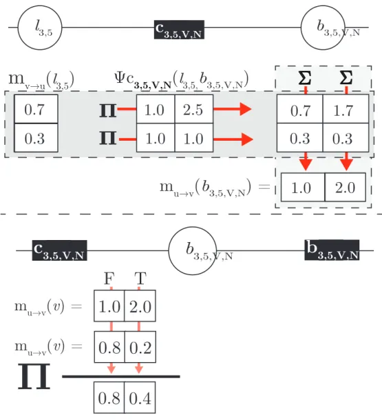
Factor graphs provide a solution to this problem. Instead of constraining variable con-figurations using many factors over small sets of variables, a single globally-connected special-purposecombinatorial factor can enforce this constraint. Such a factor encapsu-lates a function, different from standard inference procedure, to update the values of all syntactic variables simultaneously. This can be done in a much more efficient manner by leveraging dynamic programming algorithms developed earlier in the parsing literature, requiring only O(n3) time. We make use of this strategy throughout this thesis to
effi-ciently represent structured models, primarily syntactic models, and present a novel factor for efficiently representing phrase structure syntax (Sec. 3.1.2.1).
Special-purpose factors are also useful in constructing joint models. We define Boolean logic factors to coordinate between corresponding variables from separate component mod-els. For instance, if an SRL dependency commonly corresponds to a syntactic dependency, we can model a correlation between the two corresponding variables by connecting them with a Boolean logic factor. These factors contribute a score when the Boolean logic is vi-olated. This score can be derived from a set of feature weights, so the model can learn how strongly these variables correlate. While there may be many such factors used in modeling the connections between two models, each connecting factor is associated with different features and will contribute a context-sensitive score to the model.
1.2.3 Inference
During training, maximum likelihood estimation is used to find the parameters for which the model most accurately predicts the data. In order to efficiently search the vast space of all real-valued parameters, we use gradient-based optimization, which in turn re-quires computing the gradient of the model parameters. This gradient is a ratio between expectations – one expectation taken deterministically from the labeled training data, a second expectation calculable via inference. Inference in a factor graph produces factor
marginals, sometimes called beliefs. A factor’s marginal defines a distribution over the values of its neighboring variables, and is calculated by summing over them, the same marginalization process discussed earlier in Section 1.1.2 (pg. 10).
It follows that in order to compute the marginal for a single factor, all other factors must be involved in the computation. To compute the marginal for a second factor, nearly all of the same factors will be used in an identical manner. A more attractive solution is offered by message passing algorithms, a family of inference algorithms for graphical models that operate by distributing and collecting information across the graph. The key insight of message passing inference is that these otherwise redundant calculations can be cached locally, allowing for exact inference in just two passes through chain or tree-shaped graphs. For general graphs inference is intractable, but it can be approximated using loopy belief propagation, an inference method used repeatedly in this thesis.
Wrapping inference inside a gradient-based learning scheme is a common approach to supervised training, but to realize the goal of training in the presence of latent variables, as described in Eq. ??, we only need to slightly modify this procedure. Instead of acquir-ing the first expectation entirely from labeled trainacquir-ing data, this too can be calculated (or approximated, in cyclic graphs) via inference. For this calculation the subset of observed variables are set to their true values prior to inference. Inference and gradient calculations can then be performed normally, with the resulting update reflecting a marginalization over latent variables whose true values were provided by the training data. By utilizing this
two-step inference procedure inside gradient-based optimization we are able to train in the presence of latent variables, optimizing all model parameters toward the goal of improving end task performance.
1.3
A Comparison of Approaches to Joint NLP
The NLP community has made great strides in improving the performance of NLP models on single tasks, but the real-world success of these models will hinge on how well such models work together in the context of an end-to-end NLP system. In response to this need, model combination has received a great deal of attention in recent years. We divide these contributions into two groups along the conceptual axis of whether the models are trained independently and combined only during testing (joint decoding), or if they are treated jointly throughout (joint training). Common to all combination methods is the need to communicate or negotiate between model components. However, how models exchange information is unique to each approach.
1.3.1 Joint Decoding
Perhaps the simplest method of combining models is to train them independently and aggregate their output in a manner that solves the global problem. We refer to this class of approaches asjoint decodingmethods.
1.3.1.1 Comparisons to Pipeline Decoding withn-best Lists
As discussed previously, one of the most straightforward methods of model combina-tion is then-best pipeline, in which each model is processed in sequence, the output of one model – a set containing thenmost probable analyses – becoming the input to the next. In Section 1.1.1 we provided a high-level overview of why an marginalization-based decoding scheme may be preferable alternative, but having now introduced the machinery by which we implement and train our models, we discuss the remaining advantages of our approach:
(1) unidirectional vs. multidirectional information flow, and (2) passing complete analyses vs. beliefs overpartsof analyses.
1.3.1.2 Unidirectional vs. Bidirectional Information Flow
Recall that the pipeline approach fails when the optimal local solution falls outside of the n-best list. Passing forward a poor set of analyses provides a faulty foundation from which to make the next stage of predictions, leading to increasingly poorer predictions as information moves through the pipeline. One solution to this problem is to increase the size of n, making it more likely that the optimal local solution is contained within the larger list. In practice this strategy is rarely helpful, as even increasing the list capacity to hold thousands of elements rarely makes a significant difference when the list items are heavily structure objects with an enormous number of possible structures, like trees (Huang and Chiang, 2005). The larger problem is that information in a pipeline only flows in one direction.
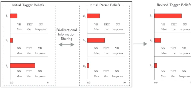
This is a handicap not shared by other approaches. For instance, a joint model can circumvent these issues because each component model’s contribution accounts for only part of the global model’s final solution. In this sense, joint inference acts as a discourse in which all models participate. Like a jury slowly nudging a dissenter toward a unified con-sensus, inference has the effect of mitigating the weaker sources of conflicting information. Let us consider how a joint model might recover from a poor local analysis in the con-text of a joint part-of-speech tagging and dependency parsing model. The sentence “Man
the harpoons.” is lexically ambiguous: both man and harpoons can be either nouns or
verbs. Consider a simple tagging model, a unigram model, which contains no dependen-cies between adjacent tags. Each word receives its most frequent tag. The word “man” is not frequently a verb, so the model would incorrectly assign the most probability to analyses where it is labeled a noun (Fig. 1.4,left).
Man the harpoons VB DET NN
Man the harpoons NN DET VB
Man the harpoons NN DET NN
0.0 1.0
Man the harpoons VB DET NN
Man the harpoons NN DET VB
Man the harpoons NN DET NN
0.0 1.0
Man the harpoons VB DET NN
Man the harpoons NN DET VB
Man the harpoons NN DET NN
0.0 1.0
Revised Tagger Beliefs Initial Parser Beliefs
Initial Tagger Beliefs
Bi-directional Information Sharing a1 a2 a3 a1 a2 a3 a1 a2 a3
Figure 1.4.Bidirectional information flow via belief propagation. The figure depicts three analyses over tag sequences (a1,a2, and a3) as scored by models prior to global inference
(left and middle) and after (right). In a traditional NLP pipeline information flows in only
one direction: forward. When a component suggests a poor analysis early in the pipeline, as is the case when taking the 1-best analysis of the tagger (left), downstream models (the parser, middle) are more likely to make poorer predictions, and errors multiply. A joint model (depicted within the bounding box) can circumvent confident, erroneous model-ing components by allowmodel-ing information to flow backwards in the pipeline, and influence earlier models. The resulting tagger beliefs favor the analysis most compatible with both models’ beliefs (right).
However, a parser scores trees based on a separate set of criteria. For instance, a parser may assign a very low score to a tree that contains no verb, as verbs play an important syntactic role and trees without them are uncommon (Fig. 1.4,middle). Thus an analysis that was initially considered very probably under the tagger becomes very unlikely when placed in the larger context. If these components were connected in a 1-best pipeline, the system would already be committed to the incorrect tag sequence and leave successive components little chance to recover. In the Fig. 1.4 example, the resulting parse,a3, would
be highly unlikely.
A joint model circumvents this by allowing information to flow in both directions. Dur-ing inference, the beliefs that a factor has over its neighbors propagate throughout the
ging and parsing, the model’s beliefs over syntactic variables can help guide its beliefs over part-of-speech variables, and vice versa. In essence, joint inference entirely discards the notion of a serialized order that was inherent in the pipeline. When inference ends and the model beliefs have converged to a globally-informed optimum, the resulting solution may differ from either the tagger or parser’s single most probable independent analysis (Fig.
1.4,right), but will reflect the pooled information of all component models.
1.3.1.3 Units of Exchange
A second point of divergence is scope of the information that is passed between models. In an n-best pipeline the model components pass forward lists of complete structures. If the model is a tagger, a list of complete tag sequences is pushed forward. If the model is a parser, a list of trees. In doing so,n-best lists force the system to multiply out ambiguities. A joint factor graph model can differ in this respect, as it can coordinate component models on a much finer level of granularity. In the method we propose, it is not models that share information, as much as itparts of modelsthat share information. Assume there is a model of syntax and a model of semantic role labeling. Coordination between these models occurs at the level of corresponding variables. If we believe that a syntactic span over a pair of indices is correlated with an SRL relationship over those indices, the variables representing these structures can be connected via a factor.
During inference, the information shared between component models takes the form of variable-to-variable interactions. A variable from one model, the source, sends a message to the coordinating factor. This message represents the variable’s belief about its values in light of all the evidence it has received from all of its other neighbors. The coordinat-ing factor receives this message and multiplies in its own score before relaycoordinat-ing it to the destination variable in the opposing model. This score either reflects the modeler’s intu-ition regarding the nature of the coordinated variables, and we consider the special case where this intuition is captured by a Boolean logic relationship, or it could alternatively
be learned entirely from data. The process of coordinating between component models in factor graphs is described in Section 2.4.3 (pg. 65).
While an n-best list might also pass forward additional information to better describe the model’s distribution, fine-grained information is still lost. For example, in a pipeline a parser may push forward a list of treesand their associated probabilities, but the weights of substructures within each tree are lost. This would be similar to classifier stacking, where each model outputs a posterior distribution instead of a finite subset of possible analyses. If knowledge of a particular substructure is useful to the end task prediction, much of this information may be lost by then-best approximation.
For instance, in SRL, in determining whether a semantic dependency exists between two words it is useful to know if there is a corresponding syntactic dependency between them. When considering the model’s beliefs over all trees, it may be very likely that this dependency exists in the tree, but this is no guarantee that it will be present in the trees selected for then-best list. This is not true of our joint approach, where the corresponding syntax and SRL variables can be directly connected in the graph. During inference, the information sent from the syntactic variable to the SRL variable represents precisely what is desired: the syntax model’s total belief that the syntactic dependency is present.
This also affects the scalability of these models. For a combinatorial structure, like a syntax tree, the number of possible trees for a given sentence length can be exceedingly large. This is often an intractable number to pass forward, and motivates approximations where only a subset of the total number of trees, then-best, are exchanged. It’s the fine-grained nature of connecting model variables rather than models, that allows our approach to remain tractable without approximations.
1.3.1.4 Other Approaches to Joint Decoding
Our approach is not the first method to solve the joint decoding problem. In this section we discuss two alternatives: Integer Linear Programming, and Dual Decomposition.
1.3.1.4.1 Integer Linear Programming
Integer linear programming (ILP) is a form of mathematical optimization which can be used to perform global inference across a set of component models. ILP maximizes a linear objective function, and requires each model (and the relationships between them) be expressed as a set of linear constraints. ILP is NP-hard but tractable for many problems, and when solved ILP provides an exact solution.
When a model is intractable one strategy to circumventing computational inefficiency is to decompose the problem into many subproblems which may be easier to solve individ-ually. ILP provides a method for finding the global solution from a set of solvers, each solv-ing part of the problem. This strategy has been applied to dependency parssolv-ing (Riedel and Clarke, 2006), SRL (Punyakanok et al., 2004), and natural language generation (Marciniak and Strube, 2005), among others. When these subproblems are component models, ILP becomes a method of model combination, and an alternative to the pipeline approach. Roth and tau Yih (2004) show that a global decoding strategy with ILP outperforms a pipeline approach when applied to named-entity recognition and relation extraction. In SRL, a task we pursue in Chapter 6, many joint parsing and ILP systems have been proposed and are included in some of the state-of-the-art systems for this task (Punyakanok et al., 2005; Tsai et al., 2005).
Not all problems are easily expressible in terms of linear constraints. Riedel and Clarke (2006) notes that non-projective dependency parsing requires an exponential number of constraints, making ILP intractable. A similar problem occurs when expressing non-projective dependency parsing with factor graphs. Riedel and Clarke (2006) avoid this problem by incrementally introducing constraints into the model, attempting to limit the number of necessary constraints to a tractable size. In our own approach with factor graphs, we adopt the method of Smith and Eisner (2008) using combinatorial factors. This method is discussed further in Section 2.4 (pg. 54).
1.3.1.4.2 Dual Decomposition
A second and related approach is dual decomposition (DD, also known more gener-ally aslagrangian relaxation1). DD has the same theoretical underpinnings as ILP, and is another technique borrowed from the mathematical optimization literature. In DD, mod-els are coerced into agreement by adjusting Lagrange multipliers. If the exact solution is found, it also returns a guarantee of optimality.
DD has been applied to a large number of joint tasks ranging from combining depen-dency parsing and constituency parsing (Rush et al., 2010), language models with syntactic machine translation (Rush and Collins, 2011), with phrase-based translation models (Chang and Collins, 2011), CCG super tagging and parsing (Auli and Lopez, 2011), and MT align-ment models (DeNero and Macherey, 2011). As a decoding strategy, DD is an attractive framework. It’s fundamental shortcoming as it pertains to our task-directed learning frame-work is that it is currently unclear how to apply it during training, in the presence of latent variables.
There are numerous differences between these alternative joint decoding method and our proposed method. Both ILP and DD have the benefit of exactness: ILP returns an exact solution if computation terminates, and DD has a high rate of discovering and proving exact solutions in a number of NLP tasks (Rush et al., 2010). But exactness comes at a cost. ILP is NP-Hard and while the solution is guaranteed to be exact, the ILP solver may not return one in a practical amount of time. DD is also somewhat limited, requiring that subproblems have efficient solutions, and non-overlapping features (such as first order logic features and features that violate Markov assumptions) . Overcoming some of these difficulties has been addressed in previous work (Martins et al., 2011), but remains an open area of investigation.
1Dual decomposition refers to a special case of Lagrangian relaxation methods in which two or more
In contrast, while loopy belief propagation only finds approximate solutions, this ap-proximation compares favorably to DD in practice (Auli and Lopez, 2011). Graphical model representations have already been developed for many NLP problems, alleviating the need to find novel ways of representing the model in a particular framework. Models can be overlapping, and dependencies between models can be specified arbitrarily between any sets of variables.
However, the most distinguishing and most pertinent difference between these ap-proaches and the joint factor graph approach is that our method can extend beyond test time, coupling models during training as well. Joint inference during training is a crucial aspect of the framework, ultimately allowing us to achieve our goal of optimizing latent structure towards a specific end task.
1.3.2 Joint Training
In Section 2.5.2 (pg. 71) we presented a simple approach to decoding a set of dependent models, then-best pipeline, and discussed scenarios where it is unlikely to find the global maximum. Joint decoding methods like ILP and DD circumvent these shortcomings, but still assume the models have already been trained, often independently from one another and using a separate data set for each. In this scenario there may be domain mismatch be-tween data sets, and models which appear earlier in the pipeline ignore useful information from later models. In contrast, joint training optimizes all models toward a single objective. In this section we provide an overview of two methods of joint training, and contrast them with our own.
1.3.2.0.3 Combining Predictions Instead of Models
One way in which to perform joint training is not to combine models per se, but rather to combine the structures they predict. The problem then shifts from learning how to co-ordinate model components, to how to train the more complicated model. Consider the sentenceJohn saw Mary. A possible parse tree for this sentence is:
(S (NP (NN JOHN)) (VP (VBSAW) (NN MARY))).
And a corresponding named-entity span to indicate that John and Mary are named entities: (PER John) saw (PER Mary)
If one wished to pursue a joint approach to named-entity recognition and parsing, one needs only to modify the grammar used by the parser to incorporate the named-entity information. The following tree reflects the predictions of both tasks:
(S (NP (NN-PER JOHN)) (VP (VBSAW) (NN-PER MARY))).
Using standard parsing methods with this grammar produce what can be thought of as a joint analysis, with one problem cleverly nested inside of another (Finkel and Manning, 2009). But this is precisely one of the limitations of the approach: only a problem that can be conveniently described inside of another can be pursued in this manner. For NER this is an intuitive method of coupling - a named entityisa specialized noun phrase, but trying to combine two problems where dependent structures are likely to cross would not be possible with this method. For instance, prosodic information is commonly characterized as a series of breaks, or pauses, in a spoken utterance. While the prosody and syntax are correlated, Ostendorf and Veilleux (1994) notes that prosodic breaks do not always correspond to syntactic boundaries. A parse tree’s syntactic spans cannot cross, and therefore there is no way to jointly model prosody and syntax in this manner.
A second disadvantage is that when combining a task with a parser, as described above, the grammar would grow multiplicatively, as a copy of each nonterminal must be made for each of the named entity labels. While many cubic time parsing algorithms exist, n as it pertains to parsing is often very small (<40), and in practice the complexity of parsing is largely determined by the size of the grammar. Thus, from an efficiency standpoint, multi-plicative increases to the size of the grammar affect the parsing algorithm at an especially
A third disadvantage of this approach is one common to many joint models: data. In order to train the joint syntax and NER model there must be a data set jointly annotated with the structures for both tasks, as joint training hinges on learning the correlation between two tasks. In proportion to the amount of unstructured data in the world, annotated data is scarce, and jointly annotated data is still unobtainable in many languages for many pairs of tasks. Finkel and Manning (2010) show how a joint model can benefit from additional singly-annotated data. In addition to the joint model, a standalone NER model is trained on data containing only NER annotations, and a standalone parser is trained on data containing only syntax trees. During training, a prior can be used to promote agreement between the standalone and joint models. This may reduce the amount of jointly annotated data required for comparable performance, but it does not remove the need for it.
1.3.2.0.4 Learning over Constrained Latent Representations
A second approach to joint training, and perhaps the work most closely resembling our own, is the Learning over Constrained Latent Representations (LCLR) framework of Chang et al. (2010). Both LCLR and our own approach share similar goals: both aim to learn the optimal latent structure for a particular end task, where only end task annotations are observed. This removes the need for jointly annotated data. However LCLR does not define latent structure to the extent that it can be thought of as a series of intermediate models – there is only input, a latent representation, and an output. As such there are no analogous supervised correlates for this algorithm (like the pipeline approach). Our method is more general and could in theory couple more than two models, yet for the scope of this thesis the setup is identical to our own.
In LCLR the end task annotations are used to guide the induction the latent structure. Though LCLR is an attempt to improve upon the ”two stage” learning method, in which a supporting task is decoded, features are extracted from these structures, and the end task model is trained to optimize these features (essentially a two-componentn-best pipeline), it can also be thought of in two stages. In the first stage the algorithm proposes a set
of “feasible” latent representations from a given example and its end task labels. These are problem-specific, and like the systems we present these could theoretically be syntax. Previous work has focused primarily on alignments (Chang et al., 2010) and chunking (Clifton et al., 2013). Current proposals for using LCLR rely on ILP for this step, requiring that these structures are capable of being phrased as a set of linear constraints.
Features are used to score intermediary structures, and the ultimate end task predictions. Learning in LCLR attempts to optimize the parameter weights that provide high scores to intermediary representations, while minimizing loss on the end task. Each latent structure decomposes, as in our framework, into many substructures. A sentence-level alignment decomposes into an alignment between words, a parse tree (in dependency syntax) decom-poses into many pairwise relationships, and so forth. An optimal latent structure is one whose substructures correspond most directly to the correct substructures of the end task (each substructure scored via a function outputting {0,1} with respect to the end task), while providing the greatest benefit to classification accuracy. Previously SVMs have been used for learning, and thus the best latent structure is the one which is the most capable of pushing otherwise incorrect end task predictions across the decision boundary.
A key difference between LCLR and our marginalization-based approach to joint train-ing is that LCLR is more explicit in the representation of latent structure. Liken-best lists, LCLR proposes sets of complete latent structures during the first step. In the case of struc-tures with combinatorial characteristics, and therefore the potential for an intractably large number of possible latent structures, this step requires heuristic pruning to carefully tune which structures are proposed in this restricted set. And importantly, the features used for the end task classification are constructed solely from the single best latent structure. Thus the most significant difference between these methods may lie in how latent structure con-tributes to the end task predictions. In our method the set of all possible latent structure are marginalized over, whereas in LCLR this summation is a maximization.