A Stochastic Method for Estimating Imputation Accuracy

Solomon, Norman (2008) A Stochastic Method for Estimating Imputation

Accuracy. Doctoral thesis, University of Sunderland.

Downloaded from: http://sure.sunderland.ac.uk/3785/

Usage guidelines

Please refer to the usage guidelines at http://sure.sunderland.ac.uk/policies.html or alternatively

contact [email protected].

A STOCHASTIC METHOD FOR

ESTIMATING IMPUTATION

ACCURACY

Norman Solomon

School of Computing and Technology University of Sunderland

A thesis submitted in partial fulfilment of the requirements of the University of Sunderland for the degree of Master of Philosophy

The research programme was carried out in collaboration with Trends Business Research of Newcastle-Upon-Tyne

Abstract

This thesis describes a novel imputation evaluation method and shows how this method can be used to estimate the accuracy of the imputed values generated by any imputation technique. This is achieved by using an iterative stochastic procedure to repeatedly measure how accurately a set of randomly deleted values are “put back” by the imputation process. The proposed approach builds on the ideas underpinning uncertainty estimation methods, but differs from them in that it estimates the accuracy of the imputed values, rather than estimating the uncertainty inherent within those values. In addition, a procedure for comparing the accuracy of the imputed values in different data segments has been built into the proposed method, but uncertainty estimation methods do not include such procedures.

This proposed method is implemented as a software application. This application is used to estimate the accuracy of the imputed values generated by the expectation-maximisation (EM) and nearest neighbour (NN) imputation algorithms. These algorithms are implemented alongside the method, with particular attention being paid to the use of implementation techniques which decrease algorithm execution times, so as to support the computationally intensive nature of the method. A novel NN imputation algorithm is developed and the experimental evaluation of this algorithm shows that it can be used to decrease the execution time of the NN imputation process for both simulated and real datasets. The execution time of the new NN algorithm was found to steadily decrease as the proportion of missing values in the dataset was increased.

The method is experimentally evaluated and the results show that the proposed approach produces reliable and valid estimates of imputation accuracy when it is used to compare the accuracy of the imputed values generated by the EM and NN imputation algorithms. Finally, a case study is presented which shows how the method has been applied in practice, including a detailed description of the experiments that were performed in order to find the most accurate methods of imputing the missing values in the case study dataset. A comprehensive set of experimental results is given, the associated imputation accuracy statistics are analysed and the feasibility of imputing the missing case study data is assessed.

Acknowledgements

Thanks to my supervisors, Dr. Giles Oatley and Dr. Ken McGarry, for their help and support. Especially for their practical and positive suggestions for improving the structure and content of this thesis.

I would also like to thank everyone at Trends Business Research (the collaborating company) for the help and support they provided throughout the entire project lifecycle. In particular, for helping to define the project objectives and for providing the case study dataset described in chapter six.

Thanks to the UK Engineering and Physical Sciences Research Council who funded the work under the Cooperative Awards in Science and Engineering scheme.

Finally, thanks to the late Richard P. Feynman whose inspirational writings kept me going when progress was slow. Especially for the book “The Pleasure of Finding Things Out”, Feynman, (2001).

Contents

Abstract...ii

Acknowledgements...iii

1.

Introduction ... 2

1.1 Description of the Work Undertaken ...4

1.1.1 Motivation for the Work... 4

1.1.2 Objectives... 5

1.2 Description of the Proposed Imputation Evaluation Method...6

1.2.1 Informal Description of the Method... 6

1.2.2 Estimating the Predictive Power of Imputation Techniques ... 7

1.2.3 Functional Overview of the Method: Structure of the Thesis... 9

1.3 Missing Data Mechanisms ...10

1.3.1 Formal Definitions of Missing Data Mechanisms... 11

1.3.2 Informal Definitions of the MAR and MCAR Concepts... 12

1.3.3 Considering Missing Data Mechanisms in Practice ... 13

1.3.4 Solving the Missing Data Problem: Deletion or Imputation?... 14

1.4 Summary of Thesis Chapters and Contribution ...15

2.

Maximum Likelihood Imputation Via the EM Algorithm ... 17

2.1 Maximum Likelihood Estimation ...18

2.1.1 The Fundamental Concept Underpinning MLE ... 18

2.1.2 Applying MLE to Incomplete Multivariate Datasets ... 20

2.2 The Expectation-Maximization Algorithm ...21

2.2.1 History and Utility of the EM Algorithm ... 22

2.2.2 EM Imputation Algorithm Data Assumptions... 22

2.2.3 Functional Outline of the EM Imputation Algorithm... 24

2.2.4 Using the SWEEP Operator to Impute Missing Values ... 26

2.3 A New Implementation of the EM Imputation Algorithm ...30

2.3.1 Verifying the Functionality of the New EM Implementation... 30

2.4 Decreasing the Execution Time of the EM Imputation Algorithm...32

2.4.1 Factors Affecting EM Algorithm Execution Time ... 32

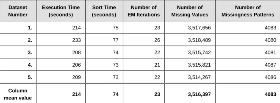
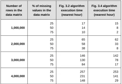
2.4.2 Measuring EM Execution Time Using Large Simulated Datasets ... 33

2.5 Summary ...36

3.

Nearest Neighbour Imputation... 38

3.1 Implementation of the NN Imputation Algorithm ...39

3.1.1 Using the Missingness Pattern Structure to Find Nearest Neighbours ... 39

3.1.2 A General Purpose Nearest Neighbour Imputation Algorithm... 40

3.1.3 Evaluating Nearest Neighbour Imputation Algorithms ... 41

3.2.1 Using the Missingness Pattern Structure to Decrease Execution Time ... 43

3.2.2 Using Donor Matrices to Speed Up NN Imputation Algorithms ... 43

3.2.3 A Fast General Purpose Nearest Neighbour Imputation Algorithm ... 45

3.2.4 Performance Evaluation Using Simulated Missing Value Datasets ... 46

3.2.5 Performance Evaluation Using Two Survey Datasets... 51

3.3 Summary ...54

4.

A Stochastic Method for Estimating Imputation Accuracy ... 56

4.1 Functional Overview of the Method ...57

4.2 Description of the Method ...57

4.2.1 Formal Description of the Method: Equations and Procedure... 58

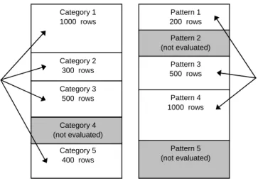
4.2.2 Estimating the Accuracy of the Imputed Values in Data Segments ... 60

4.2.3 Comparing the Accuracy of the Imputed Values in Data Segments... 63

4.3 Comparative Evaluation of Similar Methods...65

4.3.1 Similar Approaches Used by Other Researchers... 65

4.3.2 Bootstrap and Jackknife Uncertainty Estimation ... 66

4.3.3 Multiple Imputation... 68

4.3.4 Limitations of Uncertainty Estimation Methods ... 69

4.3.5 Comparing the Proposed Method with Uncertainty Estimation Methods ... 70

4.4 Summary ...72

5.

Experimental Evaluation of the Method ... 74

5.1 Assessing the Reliability and Validity of the Proposed Method...74

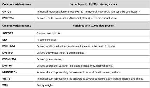
5.1.1 Description of the Dataset Used for the Experiments... 75

5.1.2 Loading the Dataset and Analysing the Variables... 76

5.1.3 Assessing the Reliability of the Method... 78

5.1.4 Assessing the Validity of the Method... 85

5.2 Comparing the Predictive Power of Candidate Imputation Methods ...91

5.2.1 Performing the Nearest Neighbour Imputation Experiments ... 91

5.2.2 Choosing the Most Accurate Imputation Method ... 93

5.2.3 Least Distortion Evaluation... 94

5.2.4 Comparing the Distortions Caused by the EM and NN Algorithms ... 97

5.3 Summary ...99

6.

Applying the Method in Practice: A Case Study ... 101

6.1 Description of the Missing Value Dataset ...101

6.2 Missingness Pattern Analysis: Defining the Missing Data Problem ...102

6.2.1 Large Proportions of Missing Data ... 102

6.2.2 Unbalanced Missingness Patterns ... 104

6.3 Addressing the Problem of Extreme Outlier Values...105

6.4.1 Using the EM Algorithm to Impute TCD Financial Values ... 109

6.4.2 Using the Nearest Neighbour Algorithm to Impute TCD Financial Values... 112

6.5 SME and LARGE Firm Financial Imputation Experiments ...115

6.5.1 Definition of the EM Imputation Experiments ... 116

6.5.2 Definition of the Nearest Neighbour Imputation Experiments... 117

6.6 Experimental Results: Estimating Imputation Accuracy ...118

6.6.1 Estimating the Accuracy of the Imputed Values ... 118

6.6.2 Estimating Imputation Accuracy in Data Segments ... 119

6.6.3 TCD Imputation Conclusions... 121

6.7 Summary ...122

7.

Conclusions and Further Work... 124

7.1 Theory and Implementation of Imputation Methods ...124

7.2 The Proposed Imputation Evaluation Method ...126

7.3 Overall Conclusions and Further Work ...128

REFERENCES... 130

APPENDICES ... 139

A TCD Imputation Experimental Results...140

B Complete EM Algorithm Pseudo-code ...154

C Software and Hardware Platform Used ...165

D Notation and Terminology Used in This Thesis ...166

List of Figures

1.1 Numeric patterns in a data matrix that has some missing values ... 7

1.2 Estimating imputation accuracy : Structure of the thesis ... 9

1.3 Data matrix illustrating the MAR and MCAR missing data mechanisms... 12

2.1 The parameters that describe a complete multivariate numeric dataset... 20

2.2 Functional outline of the EM algorithm for multivariate imputation... 24

3.1 Imputing the missing value in column 4 of row 1 in a data matrix using a NN algorithm... 39

3.2 A general purpose nearest neighbour imputation algorithm ... 41

3.3 Constructing a donor matrix for multivariate NN imputation... 44

3.4 A fast general purpose nearest neighbour imputation algorithm... 45

4.1 Functional overview of the proposed imputation evaluation method... 57

4.2 Functional outline of the repetitive, stochastic imputation evaluation process ... 59

4.3 Estimating the accuracy of the imputed values in different data segments... 60

4.4 An algorithm to perform balanced random deletions across missingness patterns ... 62

4.5 Adjusted functional outline for the proposed imputation evaluation method ... 64

4.6 Estimating imputation uncertainty using the Bootstrap method ... 66

4.7 Estimating imputation uncertainty using the Jackknife method... 67

4.8 Estimating imputation uncertainty using multiple imputation... 68

4.9 Common features of Bootstrap, Jackknife, MI and the proposed method ... 70

5.1 Implementation of the method: Data loading and variable analysis graphical user interface ... 77

5.2 Relationship between the method’s algorithm and its software implementation ... 79

5.3 Performing imputation evaluation experiments ... 80

5.4 Distribution of the RD values after imputation of DVHST94 using the EM algorithm ... 85

5.5 Deleting an “out of pattern” value - so that the imputation process can “put it back” ... 86

5.6 Distribution of the RD values after imputation of DVHST94 using the NN algorithm ... 93

5.7 Implementation of the least distortion evaluation process ... 95

5.8 Comparison of DVHST94 parameter distortions caused by the EM and NN algorithms... 97

6.1 Detecting outlier values in a perfectly normally distributed variable using Z scores... 105

6.2 Removing outlier values from the PBT distribution for approximately 1.48 million Firms... 107

6.3 Transforming the SME Payroll variable to an approximate normal distribution... 111

List of Tables

2.1 EM algorithm execution times for 5 simulated datasets containing one million rows ... 34

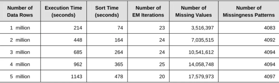
2.2 EM algorithm execution times for simulated datasets containing 1 to 5 million rows ... 35

3.1 Comparison of execution times for the two NN algorithms ... 47

3.2 Predicted execution times (to the nearest hour) for the two algorithms ... 50

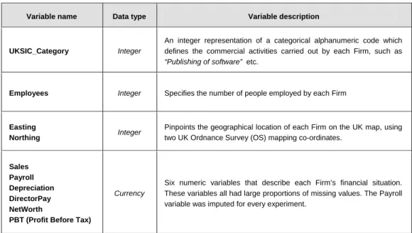
3.3 Description of the variables (data matrix columns) in the experimental datasets... 52

3.4 Comparison of algorithm execution times using segmented datasets ... 53

5.1 Description of the variables in the Canadian SSC health survey dataset ... 75

5.2 Description of SSC dataset imputation evaluation experiments 1 to 8... 78

5.3 Aggregated estimates of imputation accuracy for the SSC dataset experiments... 84

5.4 Description of SSC dataset imputation evaluation experiments 9 to 16... 91

5.5 Aggregated estimates of imputation accuracy for the SSC dataset experiments... 92

5.6 Comparison of the imputation accuracy produced by the EM and NN algorithms ... 94

6.1 Description of the variables in TBR’s missing value dataset... 102

6.2 Breakdown of proportions of missing financial data for each Firm size category... 103

6.3 Relative sizes of missingness patterns for each Firm size category ... 104

6.4 Description of financial outlier values with a robust Z score of more than ± 4... 108

6.5 Representation of the Education / Health & Social Work UKSIC categories in the TCD ... 113

6.6 Description of TCD imputation evaluation experiment 1 (EM retaining outlier Firms) ... 116

6.7 Description of TCD imputation evaluation experiment 2 (EM deleting outlier Firms) ... 116

6.8 Description of TCD imputation evaluation experiment 3 (NN retaining outlier Firms) ... 117

6.9 Description of TCD imputation evaluation experiment 4 (NN deleting outlier Firms) ... 117

Chapter One

Introduction

1.

Introduction

Non-response in surveys is perhaps the most prevalent missing data problem (Rubin, 1996a) and it is often found that several of the variables in a survey dataset - such as a set of questionnaires - have some missing values (Allison, 2001). Many statistical software packages simply omit all cases that have one or more missing values (referred to as “case deletion”) when computing the statistics that describe the dataset. This can bias the results of the data analysis process and cause misleading conclusions to be drawn, as Schafer (1997) points out;

“When the incomplete cases comprise only a small fraction of all cases (say, five percent or less) then case deletion may be a perfectly reasonable solution to the missing data problem. In multivariate settings where missing values occur on more than one variable, however, the incomplete cases are often a substantial portion of the entire dataset. If so, deleting them may be inefficient, causing large amounts of information to be discarded. Moreover, omitting them from the analysis will tend to introduce bias, to the extent that the incompletely observed cases differ systematically from the completely observed ones”

Imputation methods attempt to solve the problem of missing data by replacing missing values with plausible estimates, which avoids the problems described above. Essentially, all imputation methods have the same basic objective. That is, they try to make the best possible use of the information content (the patterns and so on) within the known values in a particular dataset, to generate the best possible estimates for the missing values in that dataset.

Rubin (1996a) points out that the primary (usually achievable) objective of imputation is to ensure that data analysis tools “can be applied to any dataset with missing values using the same command structure and output standards as if there were no missing data”, and that a further, desirable (but not always achievable) objective is to allow statistically valid inferences to be drawn when analysing imputed datasets.

Chambers (2001) lists five “desirable properties for an imputation procedure” - i.e. a set of criteria that can be used to evaluate the performance of any imputation method, as follows;

1. Predictive Accuracy - The imputation procedure should maximise preservation of true values. That is, it should result in imputed values that are "close" as possible to the true values.

2. Ranking Accuracy - The imputation procedure should maximise preservation of order in the imputed values. That is, it should result in ordering relationships between imputed values that are the same (or very similar) to those that hold in the true values.

3. Distributional Accuracy - The imputation procedure should preserve the distribution of the true data values. That is, marginal and higher order distributions of the imputed data values should be essentially the same as the corresponding distributions of the true values.

4. Estimation Accuracy - The imputation procedure should reproduce the lower order moments of the distributions of the true values. In particular, it should lead to unbiased and efficient inferences for parameters of the distribution of the true values (given that these true values are unavailable).

5. Imputation Plausibility - The imputation procedure should lead to imputed values that are plausible. In particular, they should be acceptable values as far as the editing procedure is concerned.

The list is taken directly from Chambers (2001), who explains that “The list itself is ranked from properties that are hardest to achieve to those that are easiest”. This dissertation describes a novel method for estimating the “predictive accuracy” of imputation techniques, and as such it focuses on evaluating the performance of imputation methods using the first criteria given above.

It is important to emphasise at the outset that the “true values” referred to above are the actual, real values of the missing data items, which are by definition, unknown. Therefore, it is impossible to prove that any imputation procedure has imputed values accurately, since the true values can never be compared with the imputed values. Consequently, general purpose methods for evaluating the accuracy of the imputed values generated by imputation procedures have received very little attention in the literature.

However, the accuracy of the imputed values generated by imputation procedures can

be estimated and this dissertation describes the development of a novel, general purpose

1.1

Description of the Work Undertaken

This section explains why the work was undertaken and describes how the collaboration with the partner company led to the formulation of the project objectives.

1.1.1

Motivation for the Work

The work was funded by the UK Engineering and Physical Sciences Research Council (EPSRC) under the Cooperative Awards in Science and Engineering (CASE) scheme. This scheme allows students to collaborate with commercial organisations, so that the results of the work will benefit the student, the academic institution to which that student belongs and the commercial organisation involved. In this case the work was undertaken in an attempt to solve the collaborating company’s missing data problem, as described below.

The collaborating company were Trends Business Research (TBR), who are based in Newcastle-upon-Tyne. TBR offer business and economic research consultancy to clients in the private and public sectors at local, regional, national and international levels. TBR’s activities are based upon the collection, enrichment, analysis and reporting of information describing UK business organisations, so as to further the strategic aims of their clients. This information is stored in the Trends Central Database (TCD), which describes approximately 1.48 million UK business organisations (referred to as “Firms”), ranging from sole traders to conglomerates. The TCD tables contain descriptions of each Firm, including its financial situation, number of employees, business activities and geographical location. This allows detailed statistical analysis of the data to be performed at various geographical levels - such as postcode regions or political areas, such as constituencies and wards.

However, the TCD variables that describe each Firm’s financial situation all have missing values - which constantly hampers the data analysis described above.

This problem is exacerbated by the following factors. Firstly, the proportions of missing values for each financial variable are unusually large - i.e. they range from 27 to 96 percent, depending on the variable. Secondly, 71 percent of the Firms described in the TCD have no known financial figures whatsoever (all of the values are missing). Thirdly, the missingness pattern structure (see the following section for a definition of missingness patterns) for the financial variables is extremely unbalanced. Finally, the known values for each of the financial variables all contain small proportions of very extreme outlier values.

However, the missing data problem is somewhat alleviated by the fact that larger Firms (those with more employees) generally have smaller proportions of missing financial data - i.e. the probability of a Firm’s financial figures being missing decreases as the Firm’s size increases. And some of the variables that describe each Firm are fully observed, such as the variables that specify each Firm’s geographical location. A more detailed description of the TCD dataset and TBR’s missing data problem is given in chapter six.

1.1.2

Objectives

1. To discover whether imputation of the missing values in the collaborating company’s database was feasible, given the overall poor quality of the dataset. The criterion used to assess the feasibility of the imputation process was to be the predictive accuracy of the imputed values.

2. To devise a new method for estimating the predictive accuracy of the imputed values generated by any imputation technique. The method should build on the ideas underpinning existing imputation evaluation methods.

3. To implement the method in the form of a software application that will allow users to estimate the predictive power of any imputation technique.

4. To use the software application to experimentally evaluate the reliability and the validity of the new method and to achieve the first objective.

1.2

Description of the Proposed Imputation Evaluation Method

This section gives an overview of the imputation evaluation method devised by the author (a more detailed description is given in chapter four). Section 1.2.1 gives an informal description of the method. Section 1.2.2 explains how the method can be used to estimate the predictive power of imputation techniques. Section 1.2.3 gives a functional overview of the method with reference to the contents of the rest of the thesis.

1.2.1

Informal Description of the Method

The method can be used to estimate the predictive accuracy of the imputed values for any variable in the dataset (only one variable can be evaluated each time the method is employed), where the required variable is chosen by the user of the software that implements the method. However, the evaluation process can be repeated for all of the variables in the dataset, if this is required. The functional steps of the method are summarised below.

1. A small proportion (perhaps up to 5%) of the known values are deleted at random from within the variable to be evaluated (which will already have some missing values).

2. Deleted values are recorded just before they are deleted, and a measure of how accurately they have been “put back” is taken when the imputation process is complete.

3. Steps 1 and 2 are repeated several times and the accuracy statistics computed at step 2 are stored after each repetition.

4. The stored statistics are aggregated so that the estimates of imputation accuracy produced will be more statistically reliable.

This method is described as “stochastic” in this thesis because the known values are randomly deleted at step 1. The repetition of steps 1 and 2 forms an essential part of the method, because this process will produce more statistically reliable estimates of imputation accuracy. The reason why this is true can be explained using the following example. Suppose an unbiased coin was thrown twice and fell on heads both times. A maximum-likelihood based statistical analysis of this small sample (see chapter two for a discussion of maximum likelihood theory) would estimate the probability of the coin falling on a head as 100%. However, if the coin was thrown ten times, then the estimate of the probability of a head being thrown should move closer to the true value of 50%. And as the number of throws is increased the estimate of the probability of a head being thrown should move closer and closer to the true value. This principle applies to any stochastic process which attempts to estimate unknown quantities, such as proposed imputation evaluation method

1.2.2

Estimating the Predictive Power of Imputation Techniques

The process used to estimate the predictive accuracy of imputed values is described in the previous section. This process also estimates the predictive power of the imputation technique used to generate the imputed values, which in turn allows the feasibility of using that technique to be assessed.

The proposed method also allows the predictive power of candidate imputation techniques to be compared, so that the technique that generates the most accurately imputed values can be chosen (as described in chapter five). Estimating the predictive power of an imputation technique is equivalent to measuring how well that technique has utilised the patterns within the known values in the dataset. This idea is fundamental to the proposed approach and it is discussed further below.

a b c 1 2 4 10 20 40 40 2 4 8 100 200 2 10 20 2000 4000 10 30 120

Fig 1.1 – Numeric patterns in a data matrix that has some missing values

Consider the values in the data matrix shown in Fig 1.1. The relationships between the variables (the values in the matrix columns) a, b and c are very strong, with the exception of the two “out of pattern” values (any other relationships found within the values in the Fig 1.1 matrix should be ignored here, since the idea of this section is to illustrate how data patterns would be utilised by regression based imputation procedures).

Any regression based imputation procedure should produce accurate estimates for the missing values, because the patterns within a large majority of the known values are so strong. The important point to note is that the only information available to any imputation procedure is contained within the patterns that exist among the known values in the dataset. However, these patterns will degrade and weaken as the proportion of “out of pattern” values increases, and ultimately the imputation process will become infeasible - i.e. this will occur when the proportion of “out of pattern” values exceeds a certain critical value.

Matrix cells with missing values are shaded and empty.

The relationships between the variables have a simple pattern, where;

b = a x 2 c = b x 2

These two values are “out of pattern” with the other known values.

Consider the following two extreme theoretical examples. (1) If every matrix cell with a known value contained the same value, then imputation would be easy to achieve and there would be very little uncertainty within the imputed values. (2) If every matrix cell with a known value contained a randomly generated integer in the range one to a billion, then no patterns would exist within the known values and imputation would be completely infeasible. However, in practice the patterns within most datasets will fall somewhere towards the centre of these two theoretical extremes.

Using the predictive power of the patterns in the dataset to assess imputation feasibility

The proposed method assesses the feasibility of employing a particular imputation technique by measuring how well that technique utilises the predictive power of the patterns within the known values in the dataset. That is, if the technique being evaluated by the method has been devised to utilise the type of patterns that actually do exist, then that technique should generate reasonably accurate estimates for the missing values.

The key point to note is that different types of imputation technique will utilise different types of patterns when generating estimates for missing values. For example, regression based techniques will utilise the relationships between variables to generate regression equations, whereas nearest neighbour techniques will utilise the relationships between observations to find similar matrix rows (using distance functions). However, the proposed method will work equally well regardless of the types of patterns utilised by the imputation techniques it evaluates - i.e. one of the strengths of the proposed method is that it does not need to “know” how the imputation technique it is evaluating actually works. The following example explains the reasoning underpinning this general purpose approach, with reference to the functional description of the method given in the previous section.

If imputation method X repeatedly “puts back” the randomly deleted values inaccurately, then the deleted values must not have fallen into the patterns that imputation method X used to generate estimates for the missing values. Consequently, the patterns within the known values in the dataset must not be strong enough to support imputation method X (but these patterns might be much better utilised by imputation method Y or Z, depending on how these methods work). Therefore, the feasibility of employing imputation method X to impute the missing values is questionable. This approach can be used to evaluate and compare any imputation method. The consequences of this approach are discussed in considerable detail in the more suitable context of section 5.1.4.

1.2.3

Functional Overview of the Method: Structure of the Thesis

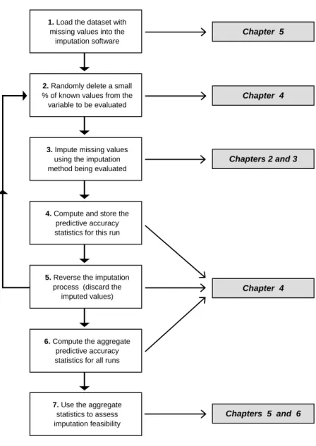
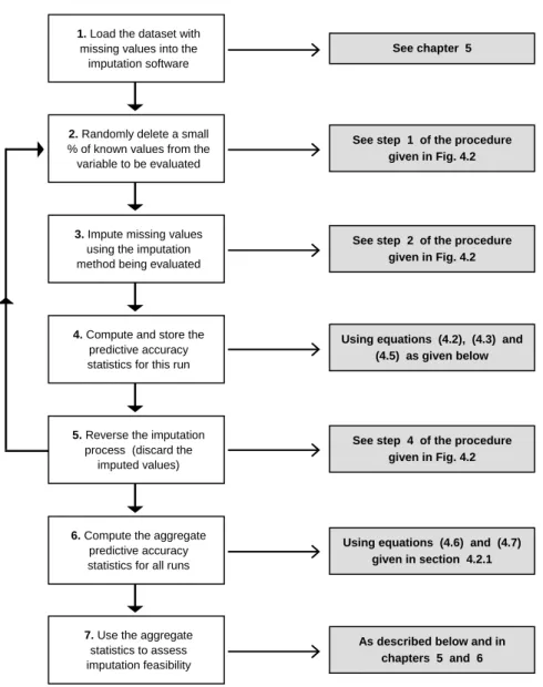
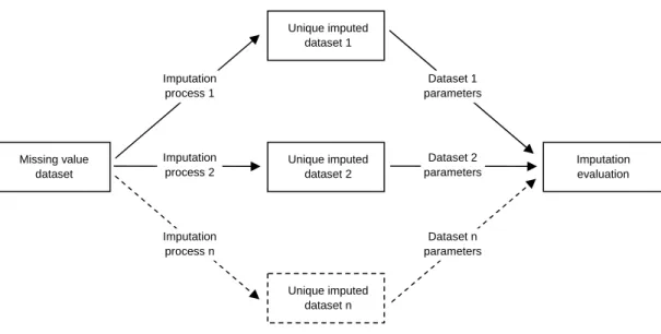
The diagram below gives an overview of the sequence of steps that are performed whenever the proposed method is employed. The overall process can be used to estimate the accuracy of the imputed values generated by any imputation technique.

Fig 1.2 – Estimating imputation accuracy : Structure of the thesis

The sequence of steps shown in Fig. 1.2 reflects the structure of the thesis. The following points are important in this respect;

•

Chapters 2 and 3 discuss the theory underpinning the imputation techniques that have been implemented as part of the software that implements the proposed method. These techniques have been implemented alongside the method in the form of an integrated software application. This was essential, because it would impractical to implement the repetitive process shown in steps 2 to 5 of Fig. 1.2 in any other way.

Chapter 4

Chapter 4

Chapters 5 and 6

1. Load the dataset with missing values into the

imputation software

2. Randomly delete a small % of known values from the variable to be evaluated

3. Impute missing values using the imputation method being evaluated This loop is

repeated several times

4. Compute and store the predictive accuracy statistics for this run

5. Reverse the imputation process (discard the

imputed values)

6. Compute the aggregate predictive accuracy statistics for all runs

7. Use the aggregate statistics to assess imputation feasibility

Chapters 2 and 3 Chapter 5

•

Chapter 4 gives a formal explanation of how the proposed method can be used to estimate the predictive accuracy of the imputed values generated by any imputation technique (e.g. the techniques described in chapters 2 and 3, among others). The ideas presented in this chapter form the principal contribution made in this dissertation.

•

Chapters 5 and 6 Chapter 5 explains how the reliability and the validity of the proposed method was experimentally evaluated. Chapter 6 assesses the feasibility of imputing the missing values in the collaborating company’s dataset.

1.3

Missing Data Mechanisms

An understanding of the “mechanisms” that lead to missing data is an essential prerequisite for an understanding of missing data problems and these ideas are referred to throughout the thesis. This section defines the terminology used when discussing missing data mechanisms, explains the theory underpinning these concepts and describes how this theory can be applied in practice.

Many imputation methods will find the most reliable estimates for missing values when these values are “missing at random” (MAR), rather than being “missing completely at random” (MCAR). These missing data patterns are referred to as “missing data mechanisms” within the literature that discusses missing data problems. Unfortunately, the nomenclature surrounding missing data mechanisms can be somewhat misleading for the uninitiated. For example, when data is said to be missing at random this means that there is some clearly identifiable patterns of “missingness” within the dataset. In other words, the probability of missing values occurring for a particular variable depends on the values of another variable (or on the values of a particular combination of the other variables in the dataset). In fact, the definitions of the MAR and MCAR assumptions have been the cause of some confusion even among statisticians, as Allison (2001) points out,

“More generally, researchers have often claimed or assumed that their data are “missing at random” without a clear understanding of what this means. Even statisticians were once vague or equivocal about this notion. However, Rubin (1976) put things on a solid foundation by rigorously defining different assumptions that might plausibly be made about missing data mechanisms”

Section 1.3.1 gives a formal summary of Rubin’s (1976) definitions - as referred to by Allison, above - and clarifies the key concept of “ignorability” for practical purposes. Section 1.3.2 attempts to clarify the concepts of MAR and MCAR using a simple illustrative dataset. Section 1.3.3 describes how missing data mechanisms are defined in practice and explains why it is impossible to prove the MAR and MCAR assumptions. Section 1.3.4 explains why it is essential to assess the feasibility of the imputation process for data that is MAR.

1.3.1

Formal Definitions of Missing Data Mechanisms

The statistical definitions of the MAR and MCAR assumptions were rigorously defined by Rubin (1976). This section gives a summary of Rubin’s definitions using a simple illustrative dataset. It can be important to refer to these definitions when discussing missing data mechanisms, to avoid misunderstandings.

Sex Income Age Sex Income Age

⎥ ⎥ ⎥ ⎥ ⎥ ⎥ ⎥ ⎥ ⎦ ⎤ ⎢ ⎢ ⎢ ⎢ ⎢ ⎢ ⎢ ⎢ ⎣ ⎡ = 64 ? 38 25000 40 38000 ? ? ? 22 ? ? 20000 F F M M M Y ⎥ ⎥ ⎥ ⎥ ⎥ ⎥ ⎥ ⎥ ⎦ ⎤ ⎢ ⎢ ⎢ ⎢ ⎢ ⎢ ⎢ ⎢ ⎣ ⎡ = 1 0 1 1 1 1 1 1 0 0 0 1 1 0 1 0 1 1 M

Consider the example given by the matrices above. Let Y be defined as a data matrix with one or more missing values in one or more of its columns, with elements represented by Yij

where the ? symbol represents a missing value. Let M be defined as a matrix of corresponding binary indicators with elements represented by Mij , such that;

1 = ij M if

Y

ij is present in Y

0

=

ij

M

if

Y

ij is missing in Y

Further, let

Y

obs represent the subset of all values present in Y, and let Ymis represent the

subset of all values missing in Y, such that Y = (Yobs ,Ymis ) represents the entire dataset

in Y. Finally, let

φ

represent a set of unknown parameters which describe the distribution in M, then;

For MAR

P

(

M

|

Y

obs

,

Y

mis

,

φ

)

=

P

(

M

|

Y

obs

,

φ

)

for all

Y

mis

,

φ

For MCAR

P

(

M

|

Y

obs

,

Y

mis

,

φ

)

=

P

(

M

|

φ

)

for all

Y

,

φ

MAR and ignorability are equivalent conditions in practice

The missing data mechanism is said to be “ignorable” - as defined by Rubin (1987) - when the data in Y is MAR, and when

φ

(the M distribution parameter) and

θ

(the Y distribution parameter) are unrelated. However, in practice, it is hard to imagine a situation where

φ

and

θ

can be related, since knowing

φ

is very unlikely to tell us anything about

θ

, and vice-versa. In addition, even in the very rare cases where

φ

and

θ

are related imputation methods should produce the same results. Essentially, this means that we can treat MAR and ignorability as equivalent conditions and that we do not need to create or process the M

1.3.2

Informal Definitions of the MAR and MCAR Concepts

Generally, when considering missing data mechanisms we are interested in finding the probability that a value will be missing, rather than attempting to impute it. This section discusses missing data mechanisms informally, using the illustrative data matrix shown below - where the missing values are represented by ? symbols.

Sex Income Age

⎥ ⎥ ⎥ ⎥ ⎥ ⎥ ⎥ ⎥ ⎦ ⎤ ⎢ ⎢ ⎢ ⎢ ⎢ ⎢ ⎢ ⎢ ⎣ ⎡ = 64 ? 38 25000 40 38000 ? ? ? 22 ? ? 20000 F F M M M Y

Fig 1.3 – Data matrix illustrating the MAR and MCAR missing data mechanisms

The missing values in a particular column are said to be MAR if the probability that they are missing is unrelated to their value, after controlling for values in the other columns. For example, suppose that 50% of the males described by the data in the Fig. 1.3 matrix failed to report their income, but only 10% of the females failed to report their income. We could then say that the probability of a person’s income being missing depended on their sex. In this case the MAR condition would be satisfied if the probability of missing income values occurring in both categories (male and female) was unrelated to the values of the income variables within those categories. Note that, by the MAR definition, the probability of a person’s income being missing could also depend on their age, or on any combination of the set of variables used to describe a person.

The missing values in a particular column are said to be MCAR if the probability that they are missing is unrelated to their value or to the values in any other column.

For example, the MCAR condition would be satisfied if the probability that the values in the income column (variable) were missing did not depend on the values in any column in the matrix, including the income column itself. When the MCAR condition is satisfied for every column in the matrix then the subset of matrix rows (observations) that have a complete set of known values can be regarded as being a random sample of all rows in the matrix. Note that the MCAR condition allows the missingness patterns in two or more columns to be related. For example, if everyone who failed to report their age also failed to report their income, then the MCAR condition could still be satisfied for the age and income variables.

1.3.3

Considering Missing Data Mechanisms in Practice

When considering alternative solutions to missing data problems it is important to realise that making an incorrect assumption about the missing data mechanism for any particular variable could devalue the results of the data analysis process. This could result in misleading conclusions being drawn, which would exacerbate the missing data problem.

“It is clear that if the imputation model is seriously flawed in terms of capturing the missing data mechanism, then so will any analysis based on such imputations. This problem can be avoided by carefully investigating each specific application, and by making best use of knowledge and data.” (Barnard and Meng, 1999)

Knowledge of the missing value dataset defines missing data mechanisms

The imputation of missing data is almost invariably a knowledge intensive process, where each missing data problem has its own unique characteristics. Consequently, the knowledge possessed by the data analyst concerning the properties of the dataset with missing values is the most important tool available when defining missing data mechanisms. For example, the dataset with missing values may have been created using the data taken from a set of returned questionnaires designed as part of a survey. In this case some questionnaires could contain missing data because some respondents failed to answer some of the questions put to them. The knowledge possessed by the designers of the questionnaire is paramount in this case, since they will understand the relationships between the variables, and consequently they will be able to define the missing data mechanism for each variable. For example, if it was known that respondents with certain characteristics (such as age or sex) were more likely to answer certain questions, then missing answers to those questions would be known to be MAR. However, if all respondents were considered equally likely to answer every question, then missing answers to all questions would be MCAR, (Barnard and Meng, 1999)

When detailed knowledge of the relationships between the variables in the missing value dataset is unavailable it can be extremely difficult to define the mechanisms that lead to missing data using diagnostic procedures alone (Graham et al, 1994). However, regression based diagnostics can sometimes be used to detect non-MCAR patterns in situations where a good linear regression model can be fitted to the data (Simonoff, 1988; Toutenburg and Fieger, 2000)

MAR and MCAR are assumptions which cannot be proved or disproved

It is very important to emphasise that the MAR and MCAR mechanisms are, by definition, assumptions which provide a conceptual framework for the analysis of missing data problems and for assessing the applicability of any particular imputation technique, and that the idea of

the most difficult idea to comprehend for those who are new to the study of missing data mechanisms, but it is the key idea underpinning this area of study. In fact, the MAR or MCAR assumption for a particular variable can never be proved - for the following reason. To prove both the MAR and the MCAR assumptions we need to prove that the probability of missing values occurring for a particular variable does not depend on the values of that variable (see Little and Rubin, 2002, among others). However, we can never prove that this supposition is either true or false, since we cannot compare the pattern in the subset of missing (unknown) values with the pattern in the subset of observed (known) values.

1.3.4

Solving the Missing Data Problem: Deletion or Imputation?

Consideration of the missing data mechanism is very important when deciding how to solve a particular missing data problem. Many statistical software applications offer the option of simply deleting all rows that have any missing values from the dataset (see for example, Nie et al, 1975). This approach is referred to as “listwise deletion” or “complete case analysis”. This can be a good solution when the missing data is MCAR and when the proportion of deleted rows is small (say up to 10%), because deleting the rows should not seriously bias the remaining data. However, when the values are MAR and the proportion of missing values is large, listwise deletion can seriously bias the remaining data, for the reasons explained below.

Consider the data matrix given in Fig. 1.3, above. Suppose that the matrix contained an equal number of male and female observations (matrix rows), and that 50% of males failed to report their income, but only 10% of females failed to report their income. In this case 30% of the rows in the data matrix would have missing values and would be deleted. But the deleted rows in the male category would represent 25% of the dataset, whereas the deleted rows in the female category would represent only 5% of the dataset. This would bias the remaining data and any subsequent analysis based on this biased data could produce misleading conclusions. In situations of this type imputation is clearly preferable to listwise deletion.

In many cases the solution to the missing data problem comes down to a choice between imputation or listwise deletion. The key question to ask when trying to make this choice is; Is the imputation process feasible? The proposed imputation evaluation method has been devised to answer this question - and it is argued that this method makes a useful contribution to imputation theory, because it can be used to assess the feasibility of imputing missing values in any numeric multivariate dataset, using any imputation method.

1.4

Summary of Thesis Chapters and Contribution

An overview of the structure of the thesis is given in Fig. 1.2, above. This section summarises the contents of the following chapters and explains how they contribute to imputation theory.

•

Chapter 2 Discusses the theory underpinning maximum likelihood based imputation and shows how this approach can be used to impute missing values in datasets with multivariate missingness patterns. The description of the author’s implementation of the expectation-maximisation algorithm, and the experiments that evaluate its performance, contribute to the theory of maximum likelihood based imputation techniques.

•

Chapter 3 Explains the ideas underpinning the functionality of a novel, fast, nearest neighbour (NN) imputation algorithm and shows how these ideas can be used to reduce the execution time of the NN imputation process. A description of the experiments that evaluate the performance of the new NN algorithm is given. The ideas and the experimental results given in this chapter contribute to NN imputation theory.

•

Chapter 4 Describes the equations and processes which form the basis of the proposed imputation evaluation method and shows how this method can be used to evaluate any imputation technique. The proposed method is compared with the most similar methods found within the literature and it is shown that the proposed method builds on the ideas underpinning these methods, but differs from them in several important respects. The descriptions and explanations given in this chapter form the principal contribution to knowledge made by this thesis.

•

Chapter 5 Explains how the proposed method was experimentally evaluated and shows that this method produces reliable and valid estimates of imputation accuracy when it is used to evaluate the imputation techniques described in chapters 2 and 3. A description of the software that implements the method is given and an explanation of how this software can be used to compare the predictive power of candidate imputation methods is provided. This chapter extends the contribution made by chapter 4 by experimentally evaluating the method which forms the principal contribution.

•

Chapter 6 Explains how the proposed method was used to address the collaborating company’s (TBR’s) missing data problem. A description of the experiments that were performed in order to find the most accurate methods for imputing TBR’s missing values is given. The experimental results are analysed and conclusions are drawn.

•

Chapter 7 Summarises the thesis, draws conclusions and describes how the work described in chapters one to six could be continued.

Chapter Two

Maximum Likelihood Imputation

Via the EM Algorithm

2.

Maximum Likelihood Imputation Via the EM Algorithm

The proposed imputation evaluation method is general purpose in nature, because it can be used to assess the feasibility of applying any imputation method to any numeric dataset. However, a “first cut” imputation method had to be implemented alongside the proposed evaluation method (in the form of an integrated software application) so that the proposed evaluation method would have an imputation method to evaluate. The imputation method that was chosen had to be general purpose in nature, in that it had to be capable of imputing missing values in any numeric dataset. Allison (2001) argues that there are only two methods of this type worth considering,

“Many alternative methods have been proposed ...Unfortunately, most of these methods have little value, and many of them are inferior to listwise deletion. That’s the bad news. The good news is that statisticians have developed two novel approaches to handling missing data - maximum likelihood estimation and multiple imputation - that offer substantial improvements over listwise deletion.”

This conclusion seems to be generally accepted among statisticians. For example, Little and Rubin (2002) - who have produced the standard reference work on missing data methods - devote the major portion of their book to a discussion of the maximum likelihood estimation (MLE) and multiple imputation (MI) methods.

The imputation method selected for the first tests of the proposed imputation evaluation method was MLE via the expectation-maximisation (EM) algorithm (Dempster, Laird and Rubin, 1977). MLE via EM was chosen in preference to MI because the MI approach can already be used to evaluate the results of the imputation process - i.e. MI is, at least in part, an imputation evaluation method, although it was designed primarily as an imputation technique. In fact, the ideas underpinning the proposed method build on the ideas underpinning MI (the similarities and differences between MI and the proposed method are described in chapter four). The following sections discuss the theory underpinning MLE and the EM algorithm, and explain how these techniques can be implemented in practice.

•

Section 2.1 explains the fundamental concept underpinning MLE and describes how the MLE approach can be used to impute missing values in multivariate datasets.

•

Section 2.2 discusses the history and utility of the EM algorithm and gives an explanation of how EM can be implemented in practice, including a description of how EM can utilise the SWEEP operator to generate regression equations.

•

Section 2.3 describes how the author has implemented the EM algorithm as a software application and explains how the functionality of the new implementation was verified

2.1

Maximum Likelihood Estimation

Section 2.1.1 gives an explanation of the fundamental concept underpinning maximum likelihood estimation (MLE), using a simple illustrative example. Section 2.1.2 explains how MLE can be applied for the imputation of missing values in incomplete multivariate datasets.

2.1.1

The Fundamental Concept Underpinning MLE

Suppose we have a biased coin, such that the probability of the coin falling on a head = 0.6, and the probability of it falling on a tail = 0.4. Then suppose that we throw this coin twice - there are four possible outcomes, as follows;

(1) Head, Head (2) Head, Tail (3) Tail, Head (4) Tail, Tail

Intuitively, we can see that, since the coin is biased towards falling on a head, outcome (1) is most probable, outcomes (2) and (3) are next (and equally) probable and outcome (4) is least probable. Stated more formally, we can say that the sequence of coin throws follows the Bernoulli distribution, such that the probability of any specific sequence of heads and tails occurring is given by;

∏

= −

−

=

n i y yi

_p

i

p

p

Y

P

1 1

)

1

(

)

|

(

(2.1)

Where Y represents a set of n throws,

y

i represents a particular throw within this set, and p gives the probability of a head occurring on any particular throw (which in this case = 0.6). For example, let 1 represent a head being thrown and 0 represent a tail being thrown. Then the probability of the occurrence of the set of throws represented by Y = {1, 1} is given by;

36 . 0 6 . 0 6 . 0 ) 6 . 0 1 ( 6 . 0 ) 6 . 0 | 1 , 1 ( 2 1 1 _{= × =} − =

∏

= − i y yi i P

Suppose that another biased coin is thrown 5 times and that it falls on a head 4 times, such that Y = {1, 1, 1, 1, 0} but this time the probability of the coin falling on a head is unknown. It follows that calculations such as the one given above cannot be performed on this set of throws, since the value of p cannot be “plugged in” to the equation. One approach to solving this problem is to find an estimate for the value of p which maximises the likelihood that the set of throws Y = {1, 1, 1, 1, 0} will occur. The process of finding the required value of p is referred to as “maximum likelihood estimation”. Stated more formally, we need to find the value of p which maximises the likelihood

L

(

p

|

Y

)

, where;

∏

= −

−

=

n i y yi i

p

p

Y

p

L

1 1

)

1

(

)

|

(

(2.2)

Notice that the right hand side of this equation is identical to the right hand side of equation (2.1) above. However, in equation (2.1) we need to find the probability that the observed data Y will occur for a given value of p. Whereas in equation (2.2) we need to find the value of p which maximises the likelihood that the observed data Y will occur. In this case we can find the required value of p by rearranging equation (2.2) so that p appears on the left hand side (the rearrangement is as given by Dunham, 2003);

∑

−

∑

=

−

=

= − = = −

∏

n i i n i i i i y n y n i y y

p

p

p

p

Y

p

L

(

|

)

(

1

)

1

(

1

)

1 1 1

Taking the log of each side (referred to as the loglikelihood) gives

)

1

log(

)

log(

)

(

log

)

(

1 1

p

y

n

p

y

p

L

p

l

n i i n i i

_⎟

⎟

−

⎠

⎞

⎜

⎜

⎝

⎛

−

+

=

=

∑

∑

= =

Then taking the derivative with respect to p gives

∑

∑

= =

−

−

−

=

∂

∂

n i n i i i

p

y

n

p

y

p

p

l

1 1

1

)

(

Finally, setting the right hand side equal to zero, to find the l (p) maximum value, gives

n y p n i i

∑

= = 1

applying this to the problem described by equation (2.2) gives

8

.

0

5

4

5

ˆ

5 1

₌

₌

=

∑

i=

y

i

p

Thus, we can say that the value of p that maximizes the likelihood of Y = {1, 1, 1, 1, 0} occurring is 0.8. It is important to emphasise that this value of p is an estimate based on single experiment with a very small sample, and that another such experiment involving 5 throws of the biased coin could easily result in a completely different sequence, such as Y = {0, 0, 0, 0, 1}. However, the same MLE approach could be applied to a much larger experimental sample (say 1000 throws) and the results would be much more reliable, but still not conclusive, since the amount of bias in the coin is unknown, and can only be estimated.

This simple example explains the central concept underpinning the MLE approach. This approach can be applied for the solution of much more complex problems than the one described above, such as the imputation of missing values in incomplete multivariate datasets, as described below.

2.1.2

Applying MLE to Incomplete Multivariate Datasets

Conceptually, the equation which gives the probability of the occurrence of any specific complete multivariate numeric dataset is similar to equation (2.1) as given in the previous section. However, the parameters that describe the multivariate distribution are much more complex, as shown in Fig. 2.1, below,

∏

= = n i i y f Y P 1 ) | ( ) | (

θ

θ

(2.3)

⎥

⎥

⎥

⎥

⎥

⎥

⎦

⎤

⎢

⎢

⎢

⎢

⎢

⎢

⎣

⎡

Σ

Σ

Σ

Σ

Σ

Σ

Σ

Σ

Σ

−

=

Σ

=

pp p p p p p p 2 1 2 22 12 2 1 12 11 1 2 1

1

)

,

(

µ

µ

µ

µ

µ

µ

µ

θ

M

O

M

M

K

L

L

Where

(

µ

1

,

µ

2

...

µ

p

)

contains the mean values for each Y column. and Σ =CSSCP n is the Y matrix covariance matrix, where; CSSCP = Corrected Sums of Squares and Cross Products matrix, as described in Tabachnick and Fidell (2000)

Fig 2.1 – The parameters that describe a complete multivariate numeric dataset

Where Y is a data matrix with all values present, θ =(µ,Σ) represents the set of parameters which describe the distribution of the data in Y and

f

(

y

i

|

θ

)

gives the probability of the occurrence of each row

y

i where i is in the range 1 to n, and n gives the number of rows in Y. Thus, the probability of the occurrence of the complete Y dataset equals the product of the probabilities of the occurrence of each row in Y.

However, we are interested in applying the MLE process to incomplete multivariate datasets, such as the Y matrix shown below. To do this we must find an estimate for the value of

θ

= (

µ

,Σ) which maximises the likelihood that the incomplete dataset in Y would occur, as we did in the example in the previous section. The first step is to specify the equation for the likelihood. Conceptually, this equation is similar to equation (2.2) given above - but some explanation of the terminology used is required before it can be presented.

⎥ ⎥ ⎥ ⎥ ⎥ ⎥ ⎥ ⎥ ⎦ ⎤ ⎢ ⎢ ⎢ ⎢ ⎢ ⎢ ⎢ ⎢ ⎣ ⎡ = 1 1 0 0 1 1 1 1 1 1 1 0 1 0 1 0 1 1 0 0 1 1 0 0 1 1 0 1 0 1 Y

Consider an incomplete data matrix such as the one shown above. Let

Y

obs represent the

subset of all values present in Y, and let

Y

mis represent the subset of all values missing in

Y, such that

Y

=

(

Y

obs

,

Y

mis

)

represents the entire dataset in Y. Now let,

)

,...

,

(

obs ,1 obs ,2 obs ,i

obs

Y

Y

Y

Y

=

represent the subset

Y

obs, where each element in

(

Y

obs,1

,

Y

obs,2

,...

Y

obs,i

)

represents the set of observed values in the corresponding row in Y. Further, let

(

µ

obs ,i

,

Σ

obs ,i

)

represent the mean and covariance matrix for a particular row i in Y, (rather than for all rows in Y, as given in equation (2.3) above). The loglikelihood based on

Y

obs is then given by,

)

|

,

(

Y

obs

l

µ

Σ

= const

(

)

(

)

2

1

ln

2

1

, , 1 1 , , , 1 , obsi obsi n i i obs T i obs i obs n i i obs

−

y

−

µ

Σ

y

−

µ

Σ

−

∑

∑

= − =

As given by Little and Rubin (2002). To impute the missing values in Y, we must find an estimate for the value of (

µ

,Σ) which maximises the likelihood of the occurrence of

Y

obs. When found, the required value of (

µ

,Σ) can be used to estimate the missing values in Y, thus completing the imputation process by producing a Y matrix with all missing values “filled in”. However, the process of finding the value of (

µ

,Σ) which maximises

)

|

,

(

Y

obs

l

µ

Σ

is complex, and the method of simply rearranging the above equation, so that

) ,

(

µ

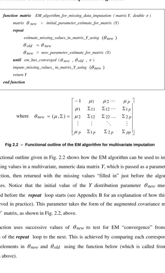
Σ appears on the left hand side - as we did for equation (2.2) - cannot be applied in this case. In fact, this maximum likelihood estimation process is so complex that an iterative procedure, such as the EM algorithm, is regarded as the simplest way to proceed (Schafer, 1997; Little and Rubin, 2002). The following sections explain how this can be achieved.

2.2

The Expectation-Maximization Algorithm

Section 2.2.1 summarises the history of the expectation-maximisation (EM) algorithm and discusses its utility. Section 2.2.2 describes the type of dataset that can be processed by the EM algorithm. Section 2.2.3 explains how the EM algorithm can be used to impute missing values in multivariate numeric datasets. Section 2.2.4 explains how the SWEEP operator can

The Y matrix has 6 rows and 5 columns

The missing values are represented by a value of 0 The present values are represented by a value of 1

2.2.1

History and Utility of the EM Algorithm

The idea of solving complex statistical problems using an iterative MLE based approach goes back as least as far as McKendrick (1926), who discusses the idea with reference to a medical application. Hartley (1958), considers the general case and develops the theory extensively, explaining many of the key concepts underpinning the entire approach. Orchard and Woodbury (1972) go on to discuss the general applicability of the approach referring to it as “the missing information principle”. Beale and Little (1975) develop these ideas further for the “multivariate normal population” by creating an “iterated form” of the method proposed by Buck (1960). The phrase “EM algorithm” first appears in the seminal paper by Dempster, Laird and Rubin (1977), who describe the fundamental properties of the EM algorithm, and discuss its general applicability to the problem of “computing maximum likelihood estimates from incomplete data”. The concepts presented in that paper sparked a revolution in the analysis of incomplete multivariate data, allowing for the efficient imputation of multivariate missing data using an iterative MLE based approach.

The EM imputation method compares very favourably with other regression based imputation methods, such as the “singular value decomposition method” (SVD) proposed by Krzanowski (1988) and the “principal component method” (PCM) proposed by Dear (1959). This conclusion has been reached by several researchers. See, for example, the useful comparative analysis of the results produced by EM, SVD and PCM given in Bello (1995), and the discussion of the application of MLE via the EM algorithm given in the standard reference book on imputation methods produced by Little and Rubin (2002).

However, the EM approach can be used for more than just imputation. In fact, the range of problems that can be addressed using EM is wide and varied, including problems which do not usually involve the analysis of missing data, as discussed by Meng and Pellow (1992) and McLachlan and Krishnan (1996), and as succinctly summarised by Schafer (1997)

“The influence of EM has been far reaching, not merely as a computational technique, but as a paradigm for approaching difficult statistical problems. There are many statistical problems which, at first glance, may not appear to involve missing data, but which can be reformulated as missing data problems: mixture models, hierarchical or random effects models, experiments with unbalanced data and many more.”

2.2.2

EM Imputation Algorithm Data Assumptions

Consider a multivariate numeric data matrix Y with one or more missing values in one or more of its columns. The EM algorithm can be used to impute the missing values in Y using an iterative, regression based procedure - assuming that the dataset is suited to the EM process. This section describes the type of dataset that can be processed by the EM algorithm

and discusses the problems that can arise when incorrect assumptions are made regarding the properties of the dataset to be processed.

The version of the EM algorithm described here will find the most reliable estimates for the missing values when all of the columns in the Y matrix are perfectly normally distributed, and when the missing values are all MAR, as described in chapter one. However, in practice, it is very unlikely that any data matrix will be perfectly normally distributed, and it will very rarely happen that the missing values in every column in the matrix are missing at random – so how should we proceed? Should we test the data to see if it is suitable to be processed by the EM algorithm? Or should we assume that the data meets requirements and run the EM algorithm immediately? The answer depends entirely on the nature of the dataset being processed and on the circumstances surrounding the particular missing data problem.

Perhaps the most sensible approach would be to proceed with the imputation process unless our knowledge of the dataset suggests that it is not suitable to be processed by the EM algorithm. For example, suppose our knowledge of the data leads us to believe that the columns in the data matrix are far from being normally distributed. To address this problem, suppose we test every column in the matrix and find that 80% of these are approximately normally distributed, with a small proportion of outliers - but that the distributions in the remaining columns are unacceptable. The decision to be made in this case is whether the 20% departure from normality invalidates the EM process, or whether it can be “worked around” or ignored. Again, everything depends on the circumstances surrounding the missing data problem. For example, the offending columns could be deleted from the matrix, but then the missing data in those columns could not be imputed, and the observed data could not be used to impute missing values in the remaining columns.

However, even in cases where some of the variables are non-normal, the EM algorithm can still produce reliable estimates for missing values (Schafer, 1997). Furthermore, in some cases variables can be transformed to approximate normality prior to imputation - e.g. using the Box-Cox algorithm described in chapter six.

The MCAR assumption complicates the EM imputation process

When values are MCAR the parameters describing the missing data pattern (represented as a binary matrix - see chapter one) must be re-estimated at each iteration of the EM algorithm. And modelling the MCAR missing data pattern is very problematic in most cases and may be impossible for some datasets. Hence, the version of the EM algorithm described below assumes that the data is MAR, since implementing an MCAR version of the EM algorithm would be extremely difficult for the reasons given above, as Allison (2000) points out;