Simplifying Maximum Flow Computations:
the Effect of Shrinking and Good Initial Flows
✩Frauke Liersa, Gregor Pardellaa
aUniversität zu Köln, Institut für Informatik, Pohligstraße 1, 50969 Köln, Germany
Abstract
Maximum-flow problems occur in a wide range of applications. Although already well-studied, they are still an area of active research. The fastest available implementations for determining maximum flows in graphs are either based on augmenting-path or on push-relabel algorithms. In this work, we present two ingredients that, appropriately used, can considerably speed up these methods. On the theoretical side, we present flow-conserving conditions under which subgraphs can be contracted to a single vertex. These rules are in the same spirit as presented by Padberg and Rinaldi (Math. Programming (47), 1990) for the minimum cut problem in graphs. These rules allow the reduction of known worst-case instances for different maximum flow algorithms to equivalent trivial instances. On the practical side, we propose a two-step max-flow algorithm for solving the problem on instances coming from physics and computer vision. In the two-step algorithm flow is first sent along augmenting paths of restricted lengths only. Starting from this flow, the problem is then solved to optimality using some known max-flow methods. By extensive experiments on instances coming from applications in theoretical physics and in computer vision, we show that a suitable combination of the proposed techniques speeds up traditionally used methods.
Keywords: maximum flow, minimum cut, subgraph shrinking, hybrid algorithm
1. Introduction
Determining maximum flows in networks is a classical problem in the area of combinatorial optimization, with many applications abound in different fields. Elegant algorithms and fast implementations are available. They allow the determination of a solution in a time growing only polynomially in the size of the input in the worst case, and large instances can be solved in practice.
We formulate the maximums-tflow problem in following. We are given a network, that is a (directed or undi-rected) graphG= (V, E). For an edgee∈Ecapacitiesce≥0are present. Further, we are given two vertices, called the sourcesand the sinkt. Letf : E →Rbe a flow function on the set of edges, and denote byfethe amount of flow on edgee. In the following we say flow and mean the corresponding flow function. We also do not distinguish between undirected edges and directed arcs, if not necessary. The value of a flow is net amount of flow out of the source. The objective is to determine a maximum flow, that is a flow with maximum value P
e∈δ+(s)
fe = P e∈δ−(t)
fe, withδ(v) =δ+(v)∪δ−(v) ={e∈E|e= (v, w)} ∪ {e∈E|e= (w, v)}. The flow has to respect the following constraints: (capacity constraints) 0≤fe≤ce,∀e∈E (1) (flow conservation) X w∈δ−(v) f(w,v)= X w∈δ+(v) f(v,w),∀v∈V \ {s, t} (2)
The set of capacity constraints (1) ensures that any feasible flow respects the capacities. The flow conservation constraints (2) avoid flow generation or elimination other than at the source and the sink. In other words, every unit
M M M M 1 v w s t
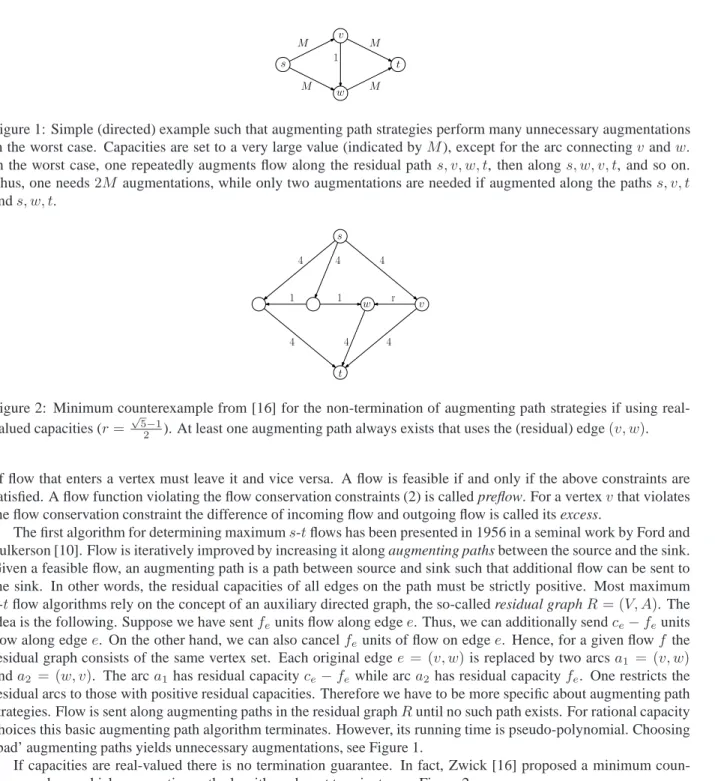
Figure 1: Simple (directed) example such that augmenting path strategies perform many unnecessary augmentations in the worst case. Capacities are set to a very large value (indicated byM), except for the arc connectingvandw. In the worst case, one repeatedly augments flow along the residual paths, v, w, t, then alongs, w, v, t, and so on. Thus, one needs2M augmentations, while only two augmentations are needed if augmented along the pathss, v, t ands, w, t. 4 4 4 4 4 4 1 1 r s t v w
Figure 2: Minimum counterexample from [16] for the non-termination of augmenting path strategies if using real-valued capacities (r= √52−1). At least one augmenting path always exists that uses the (residual) edge(v, w).
of flow that enters a vertex must leave it and vice versa. A flow is feasible if and only if the above constraints are satisfied. A flow function violating the flow conservation constraints (2) is called preflow. For a vertexvthat violates the flow conservation constraint the difference of incoming flow and outgoing flow is called its excess.
The first algorithm for determining maximums-tflows has been presented in 1956 in a seminal work by Ford and Fulkerson [10]. Flow is iteratively improved by increasing it along augmenting paths between the source and the sink. Given a feasible flow, an augmenting path is a path between source and sink such that additional flow can be sent to the sink. In other words, the residual capacities of all edges on the path must be strictly positive. Most maximum s-tflow algorithms rely on the concept of an auxiliary directed graph, the so-called residual graphR = (V, A). The idea is the following. Suppose we have sentfeunits flow along edgee. Thus, we can additionally sendce−feunits flow along edgee. On the other hand, we can also cancelfeunits of flow on edgee. Hence, for a given flowf the residual graph consists of the same vertex set. Each original edgee = (v, w)is replaced by two arcsa1 = (v, w)
anda2 = (w, v). The arca1has residual capacityce−fewhile arca2 has residual capacityfe. One restricts the
residual arcs to those with positive residual capacities. Therefore we have to be more specific about augmenting path strategies. Flow is sent along augmenting paths in the residual graphRuntil no such path exists. For rational capacity choices this basic augmenting path algorithm terminates. However, its running time is pseudo-polynomial. Choosing ‘bad’ augmenting paths yields unnecessary augmentations, see Figure 1.
If capacities are real-valued there is no termination guarantee. In fact, Zwick [16] proposed a minimum coun-terexample on which augmenting path algorithms do not terminate, see Figure 2.
Recently, Boykov and Kolmogorov [3] presented a fast implementation for determining maximums-tflows based on augmenting paths in a more elaborate way. Two search trees are used simultaneously to determine augmenting paths. One search tree starts at the source while the other is a backward tree starting at the sink. The trees are updated dynamically in each search step. This ‘double tree strategy’ yields the currently fastest implementation for instances coming from computer vision.
Dinic [4] proposed a so-called ‘blocking flow’ algorithm that can be interpreted as a clever augmenting path strategy avoiding unnecessary augmentations. Applied to the worst case from Figure 1 only two augmentations are made. This idea was independently proposed by Edmonds and Karp [5]. We note that these algorithms have strongly polynomial running time. Finally, the method with the best practical performance on general instances is the
push-relabel algorithm by Goldberg and Tarjan [8]. We describe the general idea in the ‘highest label push-push-relabel’ form. The algorithm maintains vertex labels that correspond to the distance of a vertex to the sink in the residual graph. Initially, all vertices are labeled by a BFS starting at the sink. Next, the algorithm pushes all possible flow from the source to its adjacent vertices, which results in a preflow. While the preflow is not a flow, a vertexvwith highest label is chosen among all vertices having positive excess. If possible, the excess atv is pushed along its incident edges towards the sink. If there is then still some excess left atv, the distance label ofvis updated accordingly. The push-relabel algorithm proposed by Goldberg and Tarjan [8] has strongly polynomial running time. For a detailed discussion about network flow problems and solution methods, we refer to the excellent book ‘Network Flows’ [2] and the references therein.
In the context of the minimum cut problem in undirected graphs, Padberg and Rinaldi [12] proposed conditions, amongst others, for two adjacent vertices, sayv andw, such that the minimum cut either is given by (a)δ(v), (b) byδ(w), or (c) verticesvandwbelong to the same partition. In case (c) one can safely shrink these vertices. In the context of maximums-tflows cases (a) and (b) will never occur forv,wdifferent from source and sink. Thus, the questions at hand are whether the same conditions from Padberg and Rinaldi can still be applied for maximum s-tflows, or whether there exist alike shrinking operations such that maximums-tflows are preserved. Moreover, it is interesting whether it is possible to derive conditions such that shrinking is also possible on directed graphs. We will answer these questions in the following affirmatively. On the theoretical side, we also show that these shrinking operations transform known worst-case maximums-tflow instances into trivial equivalent instances.
We aim at improving the practical running time of the fastest available implementations on instances arising in computer vision and theoretical physics. To this end, we propose in Section 2 a reduction of the input by different shrinking operations. Our operations are in the same spirit as the conditions for shrinking vertex sets that were presented in [12] by Padberg and Rinaldi for the minimum cut problem in undirected graphs. In our context, we prove the shrinking operations arguing vias-tflows in the network instead of arguing via general cuts in graphs.
Furthermore, we propose in Section 4 a hybrid maximum flow algorithm that heuristically finds a good initial flow by increasing flow along augmenting paths of restricted lengths. If the resulting flow is not maximum, the problem is solved to optimality by either a push-relabel or by an augmenting-path strategy. As the performance of these methods depends on the characteristics of the input, the specific choice of the algorithm depends on the instance’s structure.
Although the methods proposed here can in principle be applied to any instance, we expect best performance for specially structured instances. More specifically, in Section 5 we report computational results on two relevant classes of applications in which the graph of interest is a regular two- or three-dimensional grid graph where additionally each vertex is either connected to the source or to the sink. By extensive computational experiments, we find that the proposed algorithm performs very well in practice, allowing the solution of realistic instances with up to15002,
2003, and9.7∗106vertices. The outline of this work is as follows. In Section 2, we introduce the shrinking of vertex
sets. These operations are then applied in Section 3 to worst-case instances for different maximum flow algorithms. It turns out that by doing so the worst-cases can be reduced to trivial equivalent instances. Subsequently, we present the hybrid maximum flow algorithm in Section 4 and evaluate the computational results in Section 5. Finally, we conclude in Section 6.
2. Preprocessing Maximum Flow Instances
In this section we present preprocessing operations to reduce either the capacities or the input size. The optimum solutions on the modified input correspond to optimum solutions in the original input and vice versa. We will discuss the different operations on undirected as well as on directed graphs. Hence, we will mainly use terminology for undirected graphs and the directed one only when necessary. As a general preprocessing operation we suggest to remove isolated vertices, edges with capacity zero, and in the directed case vertices other than source and sink with indegree or outdegree zero. Edges connecting source and sink should also be removed. Note that the latter directly induce some amount of flow sent from the source to the sink.
2.1. Capacity Normalization
One straightforward preprocessing operation is to reduce unusable edge capacities. We call this operation capacity normalization. The latter should be applied especially when using solution methods with pseudo-polynomial running
time. Unusable capacitiescare those that cannot be exploited by any feasible flow. The corresponding edge capacities can then be reduced, as we observe next.
Observation 1. M ǫ3 ǫ2 ǫ1 v (undirected) Lete = (v, w) be the edge incident to vertexv that has largest capacity
among all edges incident tov. If it holds X
g∈δ(v)\{e}
cg≤ce,
then we can reduceceto P g∈δ(v)\{e}
cgas at most this amount of flow can be sent to and fromvusing edgee.
M ǫ3
ǫ1 ǫ2
v (directed (i) Lete= (v, w)be the arc with largest capacity with headvamong all
outgoing arcs atv. If it holds X
g∈δ−(v)
cg ≤ce,
then we can reduceceto P g∈δ−(v)
cgas at most this amount of flow can be sent tovand leavevovere.
M
ǫ3 ǫ1
ǫ2 v (directed (ii) Lete= (v, w)be the arc with largest capacity with tailvamong all
incoming arcs atv. If
X
g∈δ+(v)
cg≤ce,
then we can reduceceto P g∈δ+(v)
cgas at most this amount of flow can be sent fromvand reachvovere.
Algorithmically, capacity normalization can be accomplished by determining for each vertex the incident edge with largest capacity among all incident edges. If the condition from Observation 1 is satisfied, its capacity can be reduced accordingly. Checking the condition for all vertices takesO(|V||E|)steps. At mostO(|V|)passes are needed to ensure that all unusable capacities are removed. Thus, capacity normalization can be done inO(|V|2|E|)time. The
running time for capacity normalization is surely not competitive when compared to the running time of well-known maximums-tflow solution methods. However, if applied in a heuristic manner, for example by applying only one pass, the running time and the quality of normalization can be controlled.
2.2. Shrink Max Edge (SME)
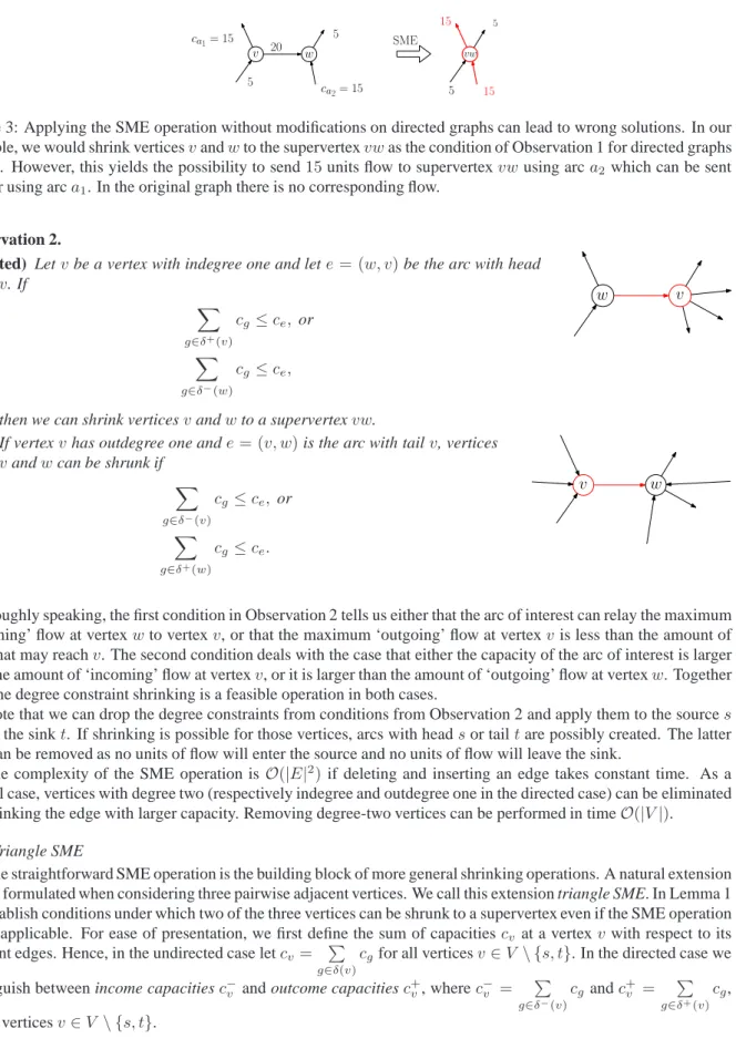
Instead of applying capacity normalizing, an edgee = (v, w)that satisfies the condition in Observation 1 can alternatively be shrunk to a supervertex by identifying its incident verticesvandw. We call this operation shrink max edge (SME). In the undirected case the condition from Observation 1 directly yields the SME condition. It is easy to see that then for each flow in the modified graph there is a corresponding flow in the original graph. Hence, an SME operation on undirected graphs preserves flow solutions. In contrast, on directed graphs this is not true, see Figure 3. Even if the condition in Observation 1 is satisfied on directed graphs shrinking may not lead to a correct algorithm. We cannot guarantee a one-to-one correspondence between flows in the modified and in the original graph. Instead, we must rephrase the condition for directed graphs. The SME operation can be applied to all verticesvwith indegree or outdegree at most one, otherwise it may lead to wrong solutions, see Figure 3. Hence, the condition now reads:
vw 20 v SME w 5 5 5 15 15 5 ca1= 15 ca2= 15
Figure 3: Applying the SME operation without modifications on directed graphs can lead to wrong solutions. In our example, we would shrink verticesvandwto the supervertexvwas the condition of Observation 1 for directed graphs is true. However, this yields the possibility to send15units flow to supervertexvwusing arca2which can be sent
further using arca1. In the original graph there is no corresponding flow.
Observation 2.
v w
(directed) Letvbe a vertex with indegree one and lete = (w, v)be the arc with head
v. If X g∈δ+(v) cg≤ce, or X g∈δ−(w) cg≤ce,
then we can shrink verticesvandwto a supervertexvw.
v w
If vertexvhas outdegree one ande= (v, w)is the arc with tailv, vertices
vandwcan be shrunk if X g∈δ−(v) cg≤ce, or X g∈δ+(w) cg≤ce.
Roughly speaking, the first condition in Observation 2 tells us either that the arc of interest can relay the maximum ‘incoming’ flow at vertexwto vertexv, or that the maximum ‘outgoing’ flow at vertexvis less than the amount of flow that may reachv. The second condition deals with the case that either the capacity of the arc of interest is larger than the amount of ‘incoming’ flow at vertexv, or it is larger than the amount of ‘outgoing’ flow at vertexw. Together with the degree constraint shrinking is a feasible operation in both cases.
Note that we can drop the degree constraints from conditions from Observation 2 and apply them to the sources and to the sinkt. If shrinking is possible for those vertices, arcs with headsor tailtare possibly created. The latter arcs can be removed as no units of flow will enter the source and no units of flow will leave the sink.
The complexity of the SME operation is O(|E|2)if deleting and inserting an edge takes constant time. As a
special case, vertices with degree two (respectively indegree and outdegree one in the directed case) can be eliminated by shrinking the edge with larger capacity. Removing degree-two vertices can be performed in timeO(|V|).
2.3. Triangle SME
The straightforward SME operation is the building block of more general shrinking operations. A natural extension can be formulated when considering three pairwise adjacent vertices. We call this extension triangle SME. In Lemma 1 we establish conditions under which two of the three vertices can be shrunk to a supervertex even if the SME operation is not applicable. For ease of presentation, we first define the sum of capacitiescv at a vertexvwith respect to its incident edges. Hence, in the undirected case letcv= P
g∈δ(v)
cgfor all verticesv∈V \ {s, t}. In the directed case we distinguish between income capacitiesc−v and outcome capacitiesc+v, wherec−v = P
g∈δ−(v)
cgandc+v = P
g∈δ+(v)
cg, for all verticesv∈V \ {s, t}.
Lemma 1.
v
w q
(undirected) Letq,v, andwbe three pairwise adjacent vertices such thatvandware different from the source and the sink. Verticesvandwcan be shrunk to a supervertex, if
2(cqv+cvw)≥cvand
2(cqw+cvw)≥cw.
v
w s
(directed (a)) Lets,v, andwbe three pairwise adjacent vertices wheresis the source. Ver-ticesvandwcan be shrunk to a supervertex, if
csv+cvw+cwv≥c+v and csw+cvw+cwv≥c+w.
v
w
t
(directed (b)) Lett,v, andwbe three pairwise adjacent vertices wheretis the sink. Vertices
vandwcan be shrunk to a supervertex, if
cvt+cvw+cwv≥c−v and
cwt+cvw+cwv≥c−w.
PROOF(LEMMA1). We prove the correctness by showing that any feasible amount of flow through supervertexvw in the modified graph has a corresponding flow with the same value in the original graph. The reverse direction is obvious. In the undirected case our argumentation is based on a local rerouting strategy. For the directed cases, the proofs rely on the fact that units of flow can be rerouted globally by rerouting them back to the source and then sending them along.
(undirected) We need to distinguish the incident edges at supervertexvwthat carry units of flow. More specifically, we distinguish between the edges incident tov andwin the original graph and show how to reroute units of flow. Further, we only consider the case in which the maximum feasible amount of flow passes supervertexvw. All other cases directly follow.
First consider the case in which there arefq,vw>0units of flow betweenqandvw. As we consider only feasi-ble flows in the modified graph it holds thatfq,vw ≤cqv+cqwandfq,vw = X
r∈N(v),w6=r6=q fvr | {z } =:fv + X r∈N(w),v6=r6=q fwr | {z } =:fw .
We routefq,vwunits of flow in the original graph to verticesvandwusing edges(q, v)and(q, w). On edge
(q, v)we route some amount of flowfqv such thatfqv ≤ cqv and on edge(q, w)we routefqw ≤ cqw units. Now, it is possible that eitherfv > fqvorfw> fqwis true. Note that both cannot be true, otherwise the flow is not feasible in the modified graph. W.l.o.g., assumefv > fqv. Hence, we must still routefv−fqvunits of flow in the original graph viawto vertexv. By the conditions in Lemma 1 it is true that
cv≤2(cqv+cvw)⇔cv−cqv−cvw | {z } ≥fv ≤ cqv |{z} ≥fqv +cvw
Therefore,fv−fqv ≤ cvw. The flow in the modified graph respects the capacity constraints, that isfq,vw ≤
cqv+cqw. Thus, if the flowfv is larger than the capacitycqvthe remaining flowfv−fqvcan be carried by edge(q, w). Thus, in the original graph we can route this amount of flow to vertexwover edge(q, w)and then tovusing edge(v, w). This completes the first case.
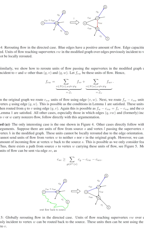
s vw csv+csw ch cl l h ? csv cvw csw v w s ch cl h l
Figure 4: Rerouting flow in the directed case. Blue edges have a positive amount of flow. Edge capacities are indicated. Units of flow reaching supervertexvwin the modified graph over edges previously incident to vertex wcannot be locally rerouted.
Similarly, we show how to reroute units of flow passing the supervertex in the modified graph using edges incident tovandwother than(q, v)and(q, w). Letfvwbe these units of flow. Hence,
fvw = X r∈N(v),w6=r6=q fvr | {z } =:fv + X r∈N(w),v6=r6=q fwr | {z } =:fw .
In the original graph we routecvwunits of flow using edge(v, w). Next, we routefw−cvwunits of flow to vertexqusing edge(q, w). This is possible as the conditions in Lemma 1 are satisfied. These units of flow are then routed fromqtovusing edge(q, v). Again this is possible asfw−cvw=fv−cvwand the conditions in Lemma 1 are satisfied. All other cases, especially those in which edges(q, vw)and (formerly) incident edges tovorwcarry nonzero flow, follow directly with this argumentation.
(directed (a)) The only interesting case is the one shown in Figure 4. Other cases directly follow with analogous arguments. Suppose there are units of flow from sourcesand vertexl passing the supervertexvw along to vertexhin the modified graph. These units cannot be locally rerouted due to the edge orientation. Hence, we cannot send units of flow from vertexwto neithersnorvin the original graph. However, we can reroute the amount of incoming flow at vertexwback to the sources. This is possible as we only consider feasible flows. Thus, there exists a path from sourcesto vertexwcarrying these units of flow, see Figure 5. Moreover, the units of flow can be sent via edgesv, as
csv≥ X
g∈δ+(v)
cg−cvw−cwv.
sent flow back to source
csv cvw csw v w s ch cl h l s vw csv+csw ch cl l h
Figure 5: Globally rerouting flow in the directed case. Units of flow reaching supervertexvw over edges previously incident to vertexwcan be routed back to the source. These units then can be sent using the edge fromstov.
q q
Z
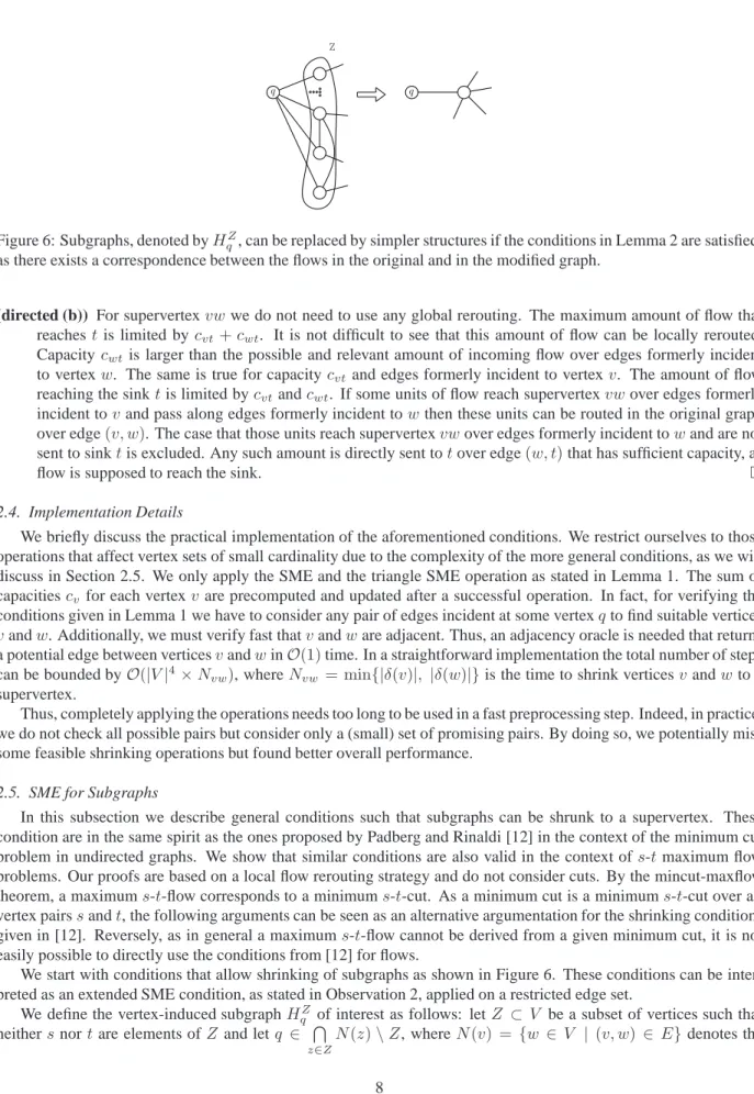
Figure 6: Subgraphs, denoted byHZ
q , can be replaced by simpler structures if the conditions in Lemma 2 are satisfied, as there exists a correspondence between the flows in the original and in the modified graph.
(directed (b)) For supervertexvw we do not need to use any global rerouting. The maximum amount of flow that reachest is limited bycvt+cwt. It is not difficult to see that this amount of flow can be locally rerouted. Capacitycwtis larger than the possible and relevant amount of incoming flow over edges formerly incident to vertexw. The same is true for capacitycvt and edges formerly incident to vertexv. The amount of flow reaching the sinktis limited bycvtandcwt. If some units of flow reach supervertexvwover edges formerly incident tovand pass along edges formerly incident towthen these units can be routed in the original graph over edge(v, w). The case that those units reach supervertexvwover edges formerly incident towand are not sent to sinktis excluded. Any such amount is directly sent totover edge(w, t)that has sufficient capacity, as
flow is supposed to reach the sink.
2.4. Implementation Details
We briefly discuss the practical implementation of the aforementioned conditions. We restrict ourselves to those operations that affect vertex sets of small cardinality due to the complexity of the more general conditions, as we will discuss in Section 2.5. We only apply the SME and the triangle SME operation as stated in Lemma 1. The sum of capacitiescv for each vertexv are precomputed and updated after a successful operation. In fact, for verifying the conditions given in Lemma 1 we have to consider any pair of edges incident at some vertexqto find suitable vertices vandw. Additionally, we must verify fast thatvandware adjacent. Thus, an adjacency oracle is needed that returns a potential edge between verticesvandwinO(1)time. In a straightforward implementation the total number of steps can be bounded byO(|V|4×Nvw), whereNvw = min{|δ(v)|, |δ(w)|}is the time to shrink verticesvandwto a
supervertex.
Thus, completely applying the operations needs too long to be used in a fast preprocessing step. Indeed, in practice, we do not check all possible pairs but consider only a (small) set of promising pairs. By doing so, we potentially miss some feasible shrinking operations but found better overall performance.
2.5. SME for Subgraphs
In this subsection we describe general conditions such that subgraphs can be shrunk to a supervertex. These condition are in the same spirit as the ones proposed by Padberg and Rinaldi [12] in the context of the minimum cut problem in undirected graphs. We show that similar conditions are also valid in the context ofs-tmaximum flow problems. Our proofs are based on a local flow rerouting strategy and do not consider cuts. By the mincut-maxflow theorem, a maximums-t-flow corresponds to a minimums-t-cut. As a minimum cut is a minimums-t-cut over all vertex pairssandt, the following arguments can be seen as an alternative argumentation for the shrinking conditions given in [12]. Reversely, as in general a maximums-t-flow cannot be derived from a given minimum cut, it is not easily possible to directly use the conditions from [12] for flows.
We start with conditions that allow shrinking of subgraphs as shown in Figure 6. These conditions can be inter-preted as an extended SME condition, as stated in Observation 2, applied on a restricted edge set.
We define the vertex-induced subgraphHZ
q of interest as follows: letZ ⊂ V be a subset of vertices such that neithersnortare elements ofZ and letq ∈ T
z∈Z
neighbourhood of nodev. The vertex-induced subgraphHZ
q , induced by{q∪Z}, is defined asHqZ ={{q} ∪Z, EqZ} withEZ
q ={(q, z)∈E |z ∈Z} ∪ {(zi, zj)∈E |zi, zj ∈ Z}. We state the necessary conditions for a shrinking operation inHZ
q in the next lemma. Lemma 2. Given a subgraphHZ
q as described above. Vertex setZcan be shrunk if ∀ ∅ 6=W ⊂Z
X w∈W,v6∈W cwv ≤2( X w∈W cqw+ X w∈W,z∈Z\W cwz) (3) holds.
PROOF(LEMMA2). We argue in an analogous way as in the proof of Lemma 1: We show how every feasible flow in the modified graph passing the supervertex can be locally rerouted in the original graph. The other direction is obvious. We suppose the considered flow is maximum.
W.l.o.g assume the SME conditions given in Observation 2 are not satisfied for any edgee∈EZ. Otherwise we first reduce vertex setZaccordingly. We start with a simple case of rerouting and then extend it to the general case. Suppose there exists a vertexz∈Z that is inHq,Z only adjacent toq. As (3) is satisfied forW ={z}, it holds that
2cqz ≥cz. Letf denote the amount of flow that passes through the supervertex using edges formerly incident to an arbitrary vertexzi∈Z\ {z}andzin the original graph. Thus in the original graph, we have to routef units of flow betweenzandzi. If vertexziis only adjacent toqin the subgraphHZ
q , then the amount of flowf betweenzandzi can be routed viaqas it holds2cqzi ≥czi, and2cqz ≥cz. Moreover, as there exists a one-to-one correspondence
between the considered edges in the modified and the original graph and the flow is feasible in the modified one, it is czi ≥f andcz≥f. This concludes the first case.
If there exists an edge(zi, zj)withzj∈ZinEZ, then the verticesq,zi, andzjform a cycle. We argue with the triangle SME conditions that in this case the flow can be rerouted betweenzandzi. Indeed, we reroutef′ = cqzi
flow units toqvia edge(q, zi)and then along(q, z)to vertexz. If there remains some units of flowf′′ =f −f′, they can be rerouted to vertexzj as2(cqzi +czizj) ≥cz ≥ f. It remains to be shown, that the remaining amount
of flowf′′can be rerouted betweenz
jandz. For now supposeziandzjare part of only one such cycle. Consider W ={zi, zj} ⊂Zthen P
w∈W,zk∈Z\W
cwzk= 0, as there exists no edge connecting vertices inZ\W with vertices in
W. Further, it is2 P
w∈W
cqw ≥cW because of (3). Therefore, we can send the remaining amount of flowf′′toqand then tozas again2cqz ≥cz≥f ≥f′′.
We assumed that verticeszi, andzj are part of only one cycle, now we drop this assumption. Hence, if vertices zi,zj orzare part of several cycles, the above argumentation is applied recursively for different choices of setW. For each set of vertices the conditions given are satisfied and thus the given amount of flow can be rerouted. The recursion is finite and either we end up with a similar situation as discussed above, that is thatzis not adjacent to any other vertex inZ, or ifzis adjacent to some vertices inZ, some amount of flow can be directly routed between those vertices without considering vertexqdue to (3). With similar arguments any combination of some feasible units of flow can be rerouted between any subsets of vertices inZ. Any possible flow betweenqand the supervertex in the
modified graph can be rerouted with similar arguments.
We argued that if conditions (3) in Lemma 2 are satisfied, then every feasible flow in the modified graph can be locally rerouted within the subgraphHZ
q , yielding a flow with the same value in the original graph. We generalize the situation in Lemma 2 to more general subgraphs.
Theorem 3. LetQ ⊂V, Z ⊂V \Qsuch that neithersnortare elements ofZ. A vertex setZ in the subgraph
HQZ= (Q∪Z, EQZ)withEQZ={(q, z)∈E |q∈Q, z∈Z} ∪ {(zi, zj)∈E|zi, zj ∈Z}andQ⊆ T
z∈Z
N(z)\Z
can be shrunk if ∀ ∅ 6=W ⊂Zand∀Y ⊆Q: X w∈W,v6∈W cwv≤2( X w∈W,q∈Y cqw+ X w∈W,v∈Z\W cwv)
Theorem 3 directly follows from Lemma 2. Moreover, the conditions in Theorem 3 are similar to conditions given by [12] in the context of minimum cuts in undirected graphs. We formalize their results in the context of maximum s-tflows in the following.
Theorem 4. LetG = (V, E)be an undirected weighted graph. LetZ be a proper subset ofV with|Z| ≥ 2such that neithersnortare elements ofZ. Further denote byN(Z)the common neighbourhood, that is the set of vertices such that every vertex inZis adjacent to every vertex inN(Z), excludingZ. If there existsY ⊆N(Z)such that for every nonempty proper subsetW ofZand for everyT ⊆Y either
(a) P w∈W,v6∈W cwv ≤2( P w∈W,v∈T cwv+ P w∈W,v∈Z\W cwv), or (b) P w∈Z\W,v6∈Z\W cwv≤2( P w∈Z\W,v∈Y\T cwv+ P w∈Z\W,v∈W cwv),
thenZ can be shrunk to a supervertex and there exists a correspondence between feasible flows in the original and the modified graph.
Theorem 4 can be understood as follows. Consider a set of verticesZ and the common neighbourhoodN(Z) = T
v∈Z
N(v)\Zin an undirected graph, see Figure 7.
T Y Z W G N(Z)
Figure 7: Schematic situation as considered in Theorem 4. SetsZ,W,Y,T, andN(Z)are shown. Black edges are those with exactly one vertex inZand the other not inW,Y, orT. Blue edges have exactly one vertex inW and the other not inZ,Y, orT. Green dotted edges connect vertices inW with those inZ\W. Purple (dashed-dotted) edges connect vertices inZ\W with those inY \T, while dark green edges connect vertices inW with vertices inT.
For a vertex set we denote by incoming amount of flow the possible amount of flow reaching this vertex set via edges with exactly one endvertex in this set. LetY be a subset ofN(Z). Now, we consider every nonempty proper subsetW ofZ. Further, for each such subset we consider every subsetT ofY. We check whether (a) the incoming amount of flow inW without the incoming amount of flow inWover edges with one endvertex inZ\W can be sent toT andZ\W or (b) the incoming amount of flow inZ\W without the incoming amount of flow over edges with one endvertex inW can be sent toW andY \T. The conditions given in Theorem 3 correspond to conditions (a) in Theorem 4. So if (a) is satisfied for all subsets, there exists a correspondence between flows in the modified and in the original graph. The second condition (b) is more sophisticated but again can be interpreted as an SME condition for subsets of edges. In the case that (a) is not satisfied for some subsetsW andT, the outgoing capacities ofW are larger than the sum of capacities of edges connectingW withT andZ\W. This may allow for feasible flows in the modified graph that cannot be realized in the original graph. However, if instead (b) is true, vertex setZcan be shrunk and the correspondence between flows in the modified and the original graph is given. Indeed, consider for example the situation in Figure 8. In the subgraph shown, the condition (a) is satisfied for allTandW, except forW ={a, b}. For this subsetW andT =Y we have:4642, and forT =∅:4630. Hence, shrinking would not be possible as
Z q c= 1 c= 5 c= 15 c= 5 c= 100 c= 10 c= 5 c= 20 Y a b c
Figure 8: A subgraph for which condition (a) of Theorem 4 is not satisfied for all considered subsetsW. Indeed, forW ={a, b}condition (a) is not satisfied for everyT. Nevertheless, setZ can be shrunk as condition (b) in 4 is satisfied for thisW. Note, we can also apply the SME condition on edge(a, b)and then on edge(ab, c)resulting in the same supervertex.
some units of flow cannot be directly rerouted viaq. However, condition (b) is satisfied forW ={a, b}and everyT. With this it is possible to reroute these units withinZand, as (a) is true for all other setsW, toq.
So, if the conditions in Theorem 4 are true for every W andT, we can shrink set Z to a supervertex. The correctness is further based on the symmetry betweenW andZ\W while considering every setTofY. Therefore, we can route the units of flow fromW toZ\W andT and then to every otherW, or vice versa the incoming flow inZ\Wcan be handled this way. With this intuitive argumentation one can state general SME conditions such that, if satisfied, a set of vertices can be shrunk to a supervertex and there exists a correspondence between feasible flows in the original and in the modified graph. It is easy to see that if a setZ has been shrunk to a supervertex and there exists some amount of flow in the modified graph that cannot be routed in the original graph, then the conditions for the corresponding setW are not satisfied. Hence, the rerouting possibilities are implicitly encoded in the conditions given in Theorem 4. Specifically one can say, if always the first condition (a) in Theorem 4 is true we already showed the one-to-one correspondence. If always the second condition (b) in Theorem 4 is true, it is easy to see that this implies that (a) is always true. So it remains to argue about the case in which (a) is not always satisfied, but instead (b). Suppose forW1,T1(a) is not satisfied but (b). Hence,
X w∈Z\W1,v6∈Z\W1 cwv≤2( X w∈Z\W1,v∈Y\T1 cwv+ X w∈Z\W1,v∈W1 cwv) (4)
This means that forW2 =Z\W1andT2=Y \T1(a) is satisfied. Consider nowW1andT2. If (a) is satisfied for
this combination, in formulae,
X w∈W1,v6∈W1 cwv≤2( X w∈W1,v∈T2 cwv+ X w∈W1,v∈Z\W1 cwv), (5)
then it is easy to see that in this case the flow can be rerouted. Suppose now, (a) is not true, but (b),
X w∈Z\W1,v6∈Z\W1 cwv≤2( X w∈Z\W1,v∈Y\T2 cwv+ X w∈Z\W1,v∈W1 cwv), (6)
which corresponds to:
X w∈Z\W1,v6∈Z\W1 cwv≤2( X w∈Z\W1,v∈T1 cwv+ X w∈Z\W1,v∈W1 cwv), (7)
that means together with (4) we can reroute every feasible amount of flow passing along edges incident to vertices in Z\W1in the original graph toY. Now considerW1andT3=Y. It is easy to see that either (a) is true or (b), which
both allows for rerouting feasible amounts of flow.
For directed graphs analogous more general conditions can be formulated as given in Lemma 1. Combining the ideas in Lemma 1 with those given in Lemma 2 the conditions follow with similar (global) rerouting arguments as used in Lemma 1.
2.5.1. Complexity of SME for Subgraphs
The general conditions presented in Section 2.5 are mainly of theoretical interest. Indeed, verifying the proposed conditions is computationally hard. Hence, it is not advisable to apply these conditions in a preprocessor for maximum s-tflow problems.
Our triangle SME conditions, given in Lemma 1, can be mapped to the special case of|Z|= 2and|Y|= 1in Theorem 4, and can be verified fast. In contrast, Padberg and Rinaldi deduce conditions from their theorem (see also Theorem 4) considering setsZof cardinality two and arbitrary large neighbourhoodY which can also be done within the flow context. More specifically, stating their theorem in the flow context, we get
Corollary 5. Letv6=w∈V \ {s, t}. If there existsY ⊆N(v)∩N(w)such that
(a) cv≤2 P u∈T∪{w} cvu, or (b) cw≤2 P u∈Y∪{v}\T cwu
holds for allT ⊆Y, then verticesvandwcan be shrunk and there exists a correspondence between feasible flows in the original and the modified graph.
For the conditions in Corollary 5 in the minimum cut context Padberg and Rinaldi remark, without giving an explicit proof, that for a givenY it is NP-complete to check the given conditions. We clarify this remark and show next that the decision problem of not shrinking is NP-complete for a givenY. First, it is easy to see that not shrinking belongs to NP. Guess a setT ⊆Y and verify in polynomial time that both conditions (a) and (b) in Corollary 5 do not hold. Next, we show that not shrinking is NP-hard and reduce the NP-completePARTITION PROBLEM[6] to the problem at hand. The latter is defined as: given a set ofnintegersS={s1, s2, . . . , sn}, withM =
n
P
i=1
si. Does a subsetR⊂S exist such that
1 2 n X i=1 si= M 2 = X si∈R si= X si∈S\R si?
For a givenPARTITIONinstance define the graph as shown in Figure 9. For every integersiwe have a vertex.
Additionally, we have a vertexvand a vertexwsuch that both are adjacent to every vertexsi. Set the capacities for the edges(v, si)and(w, si)as si
2. Vertexv is connected to the sourcesby an edge with capacity 1
2. Vertexwis
connected to the sinktby an edge with the same capacity 12. Now, if shrinking the verticesvandwis feasible it must hold for allT ⊆Y:
cv≤2 X u∈T∪{w} cvu ⇔ M + 1 2 ≤2 X si∈T si 2, or cw≤2 X u∈Y∪{v}\T cwu ⇔ M + 1 2 ≤2 X si∈Y\T si 2.
s1 s2 s3 s4 sn v w Y =N(v)∩N(w) c=s1 2 c=sn 2 c=s2 2 s t c=1 2 c=1 2
Figure 9: Corresponding flow instance graph for a givenPARTITIONinstance.
If this is true, there exists no subsetR⊂Swhich is a solution for thePARTITIONproblem. Otherwise there existsT
⊆Y such thatM2+1 >2 P si∈T si 2 and M+1 2 >2 P si∈Y\T si
2, which is a solution for thePARTITIONinstance. Therefore,
the corresponding decision problem for not shrinking is NP-complete.
3. Preprocessing Makes Worst-Case Instances Trivial
M M M M 1 s 2M t v w s t
Figure 10: Worst-case instance for augmenting path strategies and a trivial equivalent one after preprocessing the original input.
By applying the proposed preprocessing operations, well-known worst-case examples for different maximum flow algorithms can be transformed to equivalent trivial instances. Figures 10 and 11 show worst-case instances for augmenting path algorithms as given in the book by Ahuja et al. [2]. In the worst case2M augmenting steps are needed for solving the instance in Figure 10. Using non-rational capacities as in Figure 2 from [16] can even prohibit augmenting path strategies to terminate. The instance from Figure 10 can be transformed into an equivalent one by applying the triangle SME operation for directed graphs. The result is shown on the right in Figure 10. Applying shrinking operations on the dotted red cycles shown in Figure 11 and capacity normalizations on those edges yields a trivial equivalent case.
FIFO push/relabel algorithms maintain vertices with positive excess in a queue. New vertices with positive excess are added at the rear of the queue. Vertices are selected by removing them from the front of the queue. For FIFO push/relabel strategies, a worst-case instance and the trivial shrunk one are shown in Figure 12. In the worst case, the FIFO push/relabel algorithm pushes flow from the source to all adjacent vertices1,2, . . . , n−2and adds these vertices to the queue in the ordern−2, n−3, . . . ,1. The vertices are considered in this order and flow is pushed towards the sink. Only the last vertex in the queue loses its excess while all other vertices still have positive excess. Thus,n−2
4 4 4 4 4 4 1 1 r s t 4 4 4 4 8 1 r s t 4 4 8 8 1 s t 9 s t 9 9 s t 4 4 5 5 1 s t
Figure 11: Worst-case by U. Zwick [16] for augmenting path strategies, withr= √5−1
2 . Moreover, the reduction to
a trivial equivalent instance is shown. Applying SME operations and capacity-normalization on the dotted red edges yields the trivial equivalent instance.
s t M M M 1 1 1 1 n−2 1 2 n-2 s t
Figure 12: Worst-case instance for FIFO push/relabel strategy and a trivial equivalent one.
SME operations for all edges with capacityM shrinks the instance to the one shown on the right in Figure 12. As a consequence, the above worst-case instances can be solved without even calling a maximum flow algorithm. Only the proposed preprocessing operations need to be applied.
Indeed, these are small worst-case examples. Nevertheless they are commonly used to show the drawbacks of known maximum flow algorithms. Further, the presented graphs may be encountered as subgraphs in larger instances which in return can be preprocessed as shown. The proposed preprocessing operations may help in reducing the instance size independent from the used maximum flow solution method.
4. Hybrid Maximum Flow Algorithm
In this section, we propose a hybrid algorithm that starts by increasing flow through the network in a greedy fashion, using only short augmenting paths whose lengths do not exceed a certain threshold. This greedy step either finds a maximum flow or a (good) initial flow. In the latter case, the flow is increased further to an optimal one by some known maximum flow algorithm. Depending on the problem structure, we either use a lowest push/relabel approach or an augmenting path strategy. The performance of different maximum flow algorithms strongly depends on the problem structure. For example, while some approach may perform well on sparse graphs, it might take long on dense instances, or vice versa. As it is known [7] that the ‘double tree’ augmenting path strategy by Boykov and Kolmogorov [3] is especially fast on sparse instances, we use it in such cases. For dense instances, a lowest push/relabel approach performs considerably better than the ‘double tree’ procedure and is preferable in this case. We thus exploit the algorithmic advantages of the different methods. This hybrid algorithm can also be combined with preprocessing shrinking operations as presented in Section 2. After having solved the problem to optimality, all
preprocessing steps have to be undone. Finally, the optimum flow has to be rerouted accordingly. We summarize the hybrid algorithm in Algorithm 1 and discuss the greedy step in more detail next.
Algorithm 1: Hybrid maximum flow algorithm
1: (Apply preprocessing operations)
2: Label vertices
3: repeat
4: Depth-restricted flow augmentation
5: Update vertex labels afterraugmentations
6: until no augmenting path with prescribed length betweensandtis found
7: Switch to ‘double tree’ or ‘push/relabel’ strategy
8: (Undo preprocessing operations (reroute flow))
4.1. The Greedy Phase
The general idea in the depth-restricted flow augmentation phase is to label the vertices depending on the initial labels of their local neighbourhood. This yields a rough classification of the vertex set with regard to their distance fromsandt, see Figure 13. The labeling then controls a depth-restricted flow augmenting step which is performed until no augmenting path between source and sink is found. As it would take too long to determine vertex labels exactly, we only determine whether a vertex is ‘near to’ the source and/or ‘near to’ the sink or not. Intuitively, greedy augmenting paths between vertices that are far away from the source and the sink are allowed to be longer than those between vertices that are near to the source and the sink. In the following, we explain the details of this greedy step.
We assign initial vertex labelsS, T, ST, N with the following meanings. If there exists an edge(s, v)but no edge(v, t)for a vertexv, it is labeled byS. If a vertex is adjacent totbut not toswe set labelT. In case a vertex is adjacent to bothsandtlabelSTis used. If a vertex is neither adjacent tosnortit is labeled withN.
We subsequently refine the label of each vertex depending on the initial labels of its adjacent vertices. The label refinement for vertexvis independent of its own initial label, see Figure 13. Supposevis adjacent only to vertices labeled byT (resp.ST,S). Then the refined label isOT (OT,OS, respectively). Otherwise, if at least one but not all neighbours ofvare labeled byTorST, then the refined label is set toN T. Ifvdoes not have a neighbour labeled byTorST but at least one neighbour with labelS, thenvreceives the refined labelN S. In the remaining cases, the refined label is set toON. The labeling is determined by a breath-first search starting at the source and uses the initial labelsS, T, ST, Nonly. With the labeling at hand we search for augmenting paths from vertices with initial labelS. We restrict the length of those paths depending on the refined vertex label. These paths are short and can be checked fast. The labels may be updated in the residual graph after some depth-restricted augmentations and the augmenting search may be repeated.
In our experiments we found that afterr= 5augmentations, a label update should be performed. The definition of the path lengths depends on the problem at hand. Setting the thresholds to a large value increases the running time without yielding considerably better flows. Setting them to a very small threshold keeps the running time low but only yields flows with very small values. In our tests, we found good performance for the following depths: 1 (OT), 3 (N T), 7 (OS), andmin{|δ+20(s)|,14}(ON), where|δ+(s)|is the out-degree of the source in the residual graph. The
usage of long paths is prohibited for vertices with labelONif the source is only sparsely connected in the residual graph. Our computational results in Section 5 indicate that this hybrid algorithm works well on the classes of instances occurring in physics and in computer vision.
5. Computational Results
Among the many applications for maximum flows in graphs, we focus here on applications in computer vision and in theoretical physics. Although these applications are in different areas, the typical instances share a similar structure. In the random-field Ising model (RFIM) from theoretical physics, the so-called base graph is a two- or three-dimensional grid graph in which all edges have the same capacity. Furthermore, each vertex in the grid is either
sources
sinkt
adjacent to vertices with initial labelSandT
adjacent to vertices labeled byS
Figure 13: Vertex labeling and motivation for depth-restricted flow augmentation. The instances of interest show the characteristic that one can classify the vertex set into near to the source and/or near to the sink sets. Furthermore, many short paths between source and sink exists, allowing for a greedy approach as first step.
connected to an additional sourcesor to a sinktwith equal probability. The latter edges can have different capacities. Networks with a similar graph structure but different capacity choices also occur in image segmentation or image restoration applications in computer vision.
More specifically, our experiments focus on the following different instance types: (vision) directed computer vision instances [15] as reported in [3, 7] with integer capacities;
(rfim) (directed and undirected) RFIM instances as described in [13]. We used uniform interaction energy J = 1
which yields uniform capacitiesc = 1for the edges in the base graph. The random field, i.e. the capacities for edges incident to the source and the sink, was either uniform with values1,2,4,8or followed a Gaussian distribution with mean zero and variance1,2,4, and8. Grid sizes varied up to15002in 2D and up to2003in
3D.
Due to the specific structure, many cycles of length three are present in all instance classes which especially allows for the application of the triangle SME operations. We evaluate the following algorithms and implementations:
(g) highest push/relabel implementation by Goldberg and Tarjan [8] for directed graphs with integer capacities, (j) ‘mincut-lib’ by Jünger et al. [9] with a fast implementation of a ‘highest push/relabel’ algorithm for undirected
graphs,
(bk) ‘double tree’ implementation by Boykov and Kolmogorov, specialized for computer vision instances [3], (o) hybrid method with the ‘double tree’ implementation by Boykov and Kolmogorov [3] in the second step, (opr) hybrid method with our implementation of a lowest label push/relabel algorithm in the second step.
Other software libraries for maximum flows or more general minimum-cost flows exist. For example, mcf [1] can be used for these tasks. We have not included a comparison with the latter because the maximum flow program included there is basically a reimplementation of the algorithm by Goldberg and Tarjan (g). In the tables the abbreviations ((g), (j), (bk), (o), (opr)) are suffixed by ‘s’ if used on the modified graph. Computations were carried out on IntelR Xeon cCPU E5410 2.33GHz (16GB RAM) (running under Debian Linux 5.0). Some computer vision instances showed high memory requirements and thus were computed on IntelR Xeon cCPU X5680 3.33GHz (48GB RAM) and are reported separately in Table 2. Implementations (o) and (opr) are based on the graph library OGDF [11]. We marked the fastest method bold in the tables.
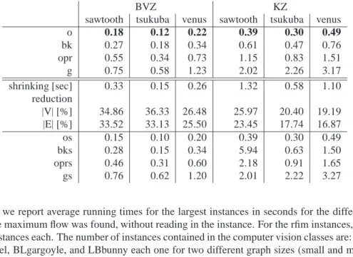
Table 1: Running times in seconds and graph reduction in % for computer vision instances. Best performance gives implementation (o). Shrinking can be executed fast and yields a considerable graph reduction. Nevertheless, the latter has no measurable influence on the running time.
BVZ KZ
sawtooth tsukuba venus sawtooth tsukuba venus
o 0.18 0.12 0.22 0.39 0.30 0.49 bk 0.27 0.18 0.34 0.61 0.47 0.76 opr 0.55 0.34 0.73 1.15 0.83 1.51 g 0.75 0.58 1.23 2.02 2.26 3.17 shrinking [sec] 0.33 0.15 0.26 1.32 0.58 1.10 reduction |V| [%] 34.86 36.33 26.48 25.97 20.40 19.19 |E| [%] 33.52 33.13 25.50 23.45 17.74 16.87 os 0.15 0.10 0.20 0.39 0.30 0.49 bks 0.28 0.15 0.34 5.94 0.63 1.50 oprs 0.46 0.31 0.60 2.18 0.91 1.65 gs 0.76 0.62 1.20 2.01 2.22 3.27
In Tables 1-6 we report average running times for the largest instances in seconds for the different solution ap-proaches until the maximum flow was found, without reading in the instance. For the rfim instances, the averages are taken over five instances each. The number of instances contained in the computer vision classes are: Liver and Baby-face one, BLcamel, BLgargoyle, and LBbunny each one for two different graph sizes (small and medium), tsukuba 16, sawtooth 20, and venus 22, see Tables 1 and 2. We report average results over each instance class. The time for shrinking is reported separately. Additionally, the resulting graph reduction is given in percent.
The computer vision instances have between105vertices,5∗105edges (BVZtsukuba) and9.7∗106vertices,
48∗106edges (BLCamel medium). The running times are small for all implementations. Often, shrinking can reduce the graphs considerably. Within short time, the sizes are reduced by about4%to46%. However, the programs often cannot profit from the reduced graph sizes as computing an optimum solution on the modified graph takes almost the same time as on the original one. Our new hybrid implementation without shrinking (o) is however considerably faster than the implementation (g). Moreover, it is the fastest method on most instances. It can even improve over the pure ‘double tree’ strategy (bk). This is remarkable as (bk) is the state-of-the-art maximum-flow implementation for instances from computer vision.
For the 2D rfim instances, there is a threshold value above which shrinking is possible. For small variances, the differences in edge capacities are too small to allow shrinking. In Tables 3-6, we show results for the largest graphs, where capacity choices are below and above the threshold. Above the threshold, shrinking can be performed fast and yields a drastic graph reduction, sometimes even by 100%. It, however, has almost no effect on the running time except when using the implementation (j) [9]. The latter needs considerably longer on the original graph, while the graph can be shrunk to a trivial equivalent instance in a few seconds. When compared to undirected instances, the shrinking steps need longer for directed graphs. For directed graphs, shrinking may be counterproductive as can be seen in Table 4. Although the graph size is drastically reduced, the total running times increases. On those instances, each augmentation step takes longer while the number of augmentations remains similar. Let us consider the implementations without shrinking. The hybrid variants perform comparable or better than the traditional algorithms on two-dimensional instances. For undirected graphs, the running time can considerably be reduced in the highest push/relabel approach when first the depth-restricted flow augmentation is applied. The situation is similar for 3D rfim instances. For directed graphs, the highest push/relabel (g) implementation is slightly faster on average than the hybrid versions. Due to memory limitations, directed instances of size2003could not be solved. We get comparable
results for instances with rational edge capacities.
For the physics instances, implementation (o) needs the same number of augmenting steps as (bk), most of them take place in the greedy step. This is also true for the directed random instances. On the other hand, on the undirected random instances (o) needs considerably less augmentation steps than (bk).
Table 2: Running times in seconds and graph reduction in % for computer vision instances with high memory require-ments. The fastest method is our (o) without shrinking on most instances. On the BLgargoyle instances implementa-tion (g) is slightly faster than our push/relabel implementaimplementa-tion. Applying the shrinking preprocessor needs negligible amount of time. However, shrinking is only possible on the small instances and again does not influence the running time significantly.
LBbunny BLgargoyle BLcamel Liver Babyface
small medium small medium small medium
o 0.51 4.39 8.78 146.11 1.59 37.72 8.33 9.04 bk 0.78 6.59 9.54 163.71 2.52 49.11 11.37 12.56 opr 1.28 18.12 4.34 99.73 4.73 89.30 21.78 31.00 g 1.72 34.11 2.93 83.29 5.69 110.31 22.16 35.57 shrinking [sec] 0.22 0.01 1.20 0.20 0.81 0.13 0.24 0.00 reduction |V| [%] 7.67 0.00 17.69 0.00 46.52 0.00 3.81 0.00 |E| [%] 6.48 0.00 16.33 0.00 43.52 0.00 3.51 0.00 os 0.50 4.48 8.69 147.50 1.38 38.09 8.00 8.97 bks 1.09 6.55 240.55 174.10 150.71 56.35 11.22 11.49 oprs 0.78 17.94 3.83 99.92 3.80 89.24 21.92 31.16 gs 1.64 36.37 3.35 88.90 5.33 149.47 24.96 37.89
Table 3: Running times in seconds and graph reduction in % for two-dimensional (2D) rfim instances, variance put in parentheses. Implementation (j) only works on undirected graphs and implementation (g) only on directed instances with integer capacities. Hence, we report for undirected graphs results of implementation (j). For directed instances we only report results of implementation (g). Our implementations (o) and (opr) show on all instances best performance. Shrinking works fast and allows for considerable graph reductions. However, the running times without the shrinking preprocessing steps show better overall performance. Although the graphs can be sometimes reduced to trivial equivalent instances the time for applying the shrinking steps is larger than the time needed to compute the maximum flow without them.
2D rfim undirected 2D rfim directed
1000 (1) 1000 (4) 1500 (1) 1500 (4) 1000 (1) 1000 (4) 1500 (1) 1500 (4) o 3.30 0.87 8.06 1.80 1.19 0.78 2.84 1.90 bk 4.93 1.29 11.17 2.91 1.46 0.95 3.40 2.21 opr 14.44 3.37 36.84 7.04 3.09 0.23 7.43 0.55 j 61.81 480.92 64.68 2492.09 g 2.98 0.25 7.72 0.58 shrinking [sec] 0.56 3.91 1.29 8.91 2.64 2.60 5.47 5.42 reduction |V| [%] 0.00 100.00 0.00 100.00 60.00 60.00 60.00 60.00 |E| [%] 0.00 100.00 0.00 100.00 54.19 54.19 54.19 54.19 os 3.44 0.01 7.97 0.02 0.82 0.54 1.96 1.35 bks 5.01 0.00 11.41 0.00 0.93 0.66 2.14 1.61 oprs 14.55 0.00 38.80 0.00 1.45 0.63 4.52 1.55 js 62.25 0.00 64.88 0.00 gs 0.57 0.68 1.35 1.69
Table 4: Running times in seconds and graph reduction in % for three-dimensional (3D) rfim instances type, variance put in parentheses, (j) for undirected and (g) for directed instances. Our implementation (o) and the pure double tree approach (bk) show good performance and are faster or comparable to implementation (g). Applying the shrink-ing preprocessor helps to reduce the overall runnshrink-ing time especially for implementation (j) on undirected instances. However, on directed instances shrinking may be even counterproductive for implementations (o), (bk), and (opr).
3D rfim undirected 3D rfim directed
150 (1) 150 (4) 200 (1) 200 (4) 100 (1) 100 (4) 150 (1) 150 (4) o 25.38 4.04 66.11 9.69 13.78 0.78 59.08 2.97 bk 23.35 5.88 58.44 13.88 21.96 0.99 105.32 3.75 opr 79.69 17.34 226.46 53.48 27.16 1.54 119.47 5.61 j 77.56 6044.08 247.27 34170.31 g 13.42 0.76 69.65 2.73 shrinking [sec] 2.23 8.42 0.45 14.69 1.91 6.37 5.79 23.79 reduction |V| [%] 0.00 70.41 0.00 46.50 2.58 60.00 1.73 60.00 |E| [%] 0.00 74.22 0.00 49.24 1.61 57.23 1.07 57.26 os 25.33 1.47 66.22 6.16 14.12 6878.12 62.31 77501.83 bks 23.18 2.05 58.40 9.59 22.76 5370.99 110.21 62283.99 oprs 79.30 3.66 226.03 18.91 26.14 2983.62 116.11 34097.49 js 77.64 458.84 246.93 9000.64 gs 13.04 0.33 68.57 1.21
Table 5: Running times in seconds and graph reduction in % for two-dimensional (2D) rfim instances with rational capacities, variance put in parentheses, (j) for undirected instances. Best performance on these class of instances shows implementation (o). Shrinking again works very fast. Except for implementation (j) the running time needed for shrinking plus the time needed to calculate the maximums-tflow on the modified graph is larger than on the original graph.
2D rfim undirected 2D rfim directed
1000 (1) 1000 (4) 1500 (1) 1500 (4) 1000 (1) 1000 (4) 1500 (1) 1500 (4) o 5.13 1.08 9.94 2.99 1.47 0.78 3.01 2.48 bk 7.30 1.52 14.90 3.78 1.65 0.89 3.75 2.54 opr 28.40 3.35 59.30 9.27 6.71 1.35 17.08 4.01 j 92.21 229.02 382.36 1268.64 shrinking [sec] 0.65 1.86 1.14 6.17 1.57 2.34 3.01 5.75 reduction |V| [%] 0.01 53.82 0.01 53.83 10.77 60.00 10.76 60.00 |E| [%] 0.01 56.08 0.01 56.09 7.93 52.44 7.92 52.43 os 5.24 0.59 9.99 1.69 1.44 0.59 3.50 1.78 bks 7.30 0.95 14.95 2.50 1.67 0.74 3.71 2.06 oprs 28.74 1.42 58.66 4.25 6.98 1.51 17.13 4.75 js 95.78 82.96 382.38 461.55
Table 6: Running times in seconds and graph reduction in % for three-dimensional (3D) rfim instances type with rational capacities, variance put in parentheses, (j) for undirected instances. The performance of the different im-plementations varies but here the double tree approaches show better overall performance. Shrinking again works very fast. Except for implementation (j) the running time needed for shrinking plus the time needed to calculate the maximums-tflow on the modified graph is larger than on the original graph.
3D rfim undirected 3D rfim directed
150 (1) 150 (4) 200 (1) 200 (4) 100 (1) 100 (4) 150 (1) 150 (4) o 46.60 9.29 182.85 50.42 107.13 1.60 720.31 5.06 bk 51.31 12.77 159.84 32.41 134.28 1.72 899.04 5.36 opr 215.53 43.67 674.84 130.22 122.76 4.44 670.39 13.94 j 119.53 3671.92 428.90 20580.39 shrinking [sec] 2.42 6.66 0.62 13.25 2.32 6.69 7.66 18.50 reduction |V| [%] 0.00 22.51 0.00 19.33 0.66 56.82 0.54 56.70 |E| [%] 0.00 24.41 0.00 20.88 0.35 46.77 0.28 46.62 os 46.28 7.02 213.64 19.08 104.80 285.72 741.43 2893.48 bks 49.84 9.91 208.60 31.35 135.04 491.93 919.38 4884.73 oprs 220.68 32.53 647.23 93.49 117.83 180.22 659.96 1969.35 js 118.59 2448.62 475.65 14797.21
Although the introduced preprocessing operations have mainly been designed for the applications mentioned above, it is interesting to evaluate them on more random instances. There are two reasons for testing the presented preprocessing operations on random graphs. Firstly, we are interested in the question whether there is a threshold con-cerning the connectivity of the source and the sink with vertices in the base graph, such that the shrinking operations are applicable. Secondly, in random graphs the probability of short augmenting paths is rare. Hence, we are interested in the question whether applying the greedy step on those instances is still worthwhile. We evaluated directed and undirected random graphs, with5∗105many vertices and varying density, generated with the graph generator rudy
[14] for the base graph. Our results confirm our conjecture, i.e. if less than50%of the vertices in the base graph are adjacent to source or sink, only few shrinking operations are possible and the graph size is only marginally reduced. This does not come as a surprise as not many potential candidates are present that satisfy the proposed SME condi-tions. On random graphs with at least50%of base graph vertices adjacent to source or sink, shrinking reduces the number of vertices considerably. For this class of instances, the proposed hybrid approach works well when com-pared to the pure double tree strategy (bk), especially on undirected instances. This observation is independent of the connectivity of the base graph. On undirected instances, the performance of (bk) can considerably be improved with the greedy step. However, especially for directed graphs, traditional methods like push/relabel algorithms, for exam-ple (g), are preferable. In general, shrinking is performed very fast on undirected instances, but takes some time on directed instances. However, in the latter case more reduction is possible. Solving the shrunk directed instances takes again longer (except with (g)), similar to the results we get for 3D rfim instances, see Table 4 (directed instances). As a consequence, it is advantageous to apply the hybrid algorithm without shrinking on undirected graphs in case the vertices in the base graph are highly connected to the source and the sink.
6. Conclusion
We proposed preprocessing operations for maximum flow problems. We showed that the input size can be reduced by applying SME operations that preserve optimal solutions. Moreover, well-known worst-case instances for different maximum flow algorithms can be transformed into trivial equivalent instances.
Subsequently, we presented a depth-restricted augmenting path algorithm that yields a good initial flow very fast. In combination with known solution strategies, the running times of traditional maximum flow algorithms are considerably reduced on relevant instances from physics and computer vision. The presented running times for the shrinking operations show that our implementation of these steps is very fast. Moreover, taking the special graph
structure into account, shrinking can remarkably reduce the graph sizes and the running time of highest push/relabel algorithms on undirected graphs. Nevertheless, shrinking has to be applied with care: For directed graphs, the running time can increase as each augmentation step takes longer. For instances from theoretical physics and computer vision, the fastest method uses augmenting path strategies without shrinking but with the new depth-restricted augmentation step as proposed here. For directed instances, the implementation (g) from [8] is the fastest one. However, it can only be used for integral capacities. As a summary, our hybrid algorithm without shrinking reduces the running time on undirected random instances that are highly connected to source and sink. Furthermore, on vision and rfim instances it even improves the method (bk) which is the currently fastest available program for sparse graphs. More specifically, the running time of the hybrid implementation with the ‘double tree’ strategy (o) is at least comparable or faster than (bk).
Acknowledgments
We are grateful to Birgit Engels for fruitful discussions and valuable comments concerning the complexity of the shrinking conditions presented in Section 2.5.1.
References
[1] MCF software package for the minimum cost flow problem. http://sorsa.unica.it/it/software.php.
[2] R. K. Ahuja, T. L. Magnanti, and J. B. Orlin. Network Flows: Theory, Algorithms, and Applications. Prentice Hall Inc., 1993.
[3] Y. Boykov and V. Kolmogorov. An Experimental Comparison of Min-Cut/Max-Flow Algorithms for Energy Minimization in Vision. IEEE Transactions on Pattern Analysis and Machine Intelligence, 26(9):1124–1137, 2004.
[4] E. A. Dinic. An Algorithm for the Solution of the Problem of Maximal Flow in a Network with Power Estimation. Doklady Akademii Nauk SSSR, 194:754–757, 1970.
[5] J. Edmonds and R. M. Karp. Theoretical Improvements in Algorithmic Efficiency for Network Flow Problems. Journal of the ACM, 19:248– 264, Apr. 1972.
[6] M. R. Garey and D. S. Johnson. Computers and Intractability, A Guide to the Theory of NP-Completeness. A Series of Books in the Mathematical Sciences. W. H. Freeman and Company, 1979.
[7] A. V. Goldberg. The Partial Augment-Relabel Algorithm for the Maximum Flow Problem. In ESA ’08: Proceedings of the 16th annual European symposium on Algorithms, pages 466–477. Springer-Verlag, 2008.
[8] A. V. Goldberg and R. E. Tarjan. A New Approach to the Maximum-Flow Problem. Journal of the Association for Computing Machinery, 35(4):921–940, 1988.
[9] M. Jünger, G. Rinaldi, and S. Thienel. Practical Performance of Efficient Minimum Cut Algorithms. Algorithmica, 26:172–195, 2000. [10] Jr. L. R. Ford and D. R. Fulkerson. Maximal Flow Through a Network. Canadian Journal of Mathematics, 8:399–404, 1956. [11] OGDF. Open Graph Drawing Framework. http://www.ogdf.net, 2007.
[12] M. Padberg and G. Rinaldi. An Efficient Algorithm for the Minimum Capacity Cut Problem. Mathematical Programming A, 47(1):19–36, 1990.
[13] H. Rieger. Optimization Problems and Algorithms from Computer Science. In R. A. Meyers, editor, Encyclopedia of Complexity and Systems Science, pages 6407–6425. Springer, 2009.
[14] G. Rinaldi. rudy – a Rudimentary Graph Generator. https://www-user.tu-chemnitz.de/~helmberg/rudy.tar.gz, 1998. [15] University of Western Ontario. Computer Vision Instances: http://vision.csd.uwo.ca/maxflow-data.
[16] U. Zwick. The Smallest Networks on Which the Ford-Fulkerson Maximum Flow Procedure May Fail to Terminate. Theoretical Computer Science, 148(1):165–170, 1995.


![Figure 11: Worst-case by U. Zwick [16] for augmenting path strategies, with r = √ 5−1 2](https://thumb-us.123doks.com/thumbv2/123dok_us/10196254.2922468/14.892.255.637.157.704/figure-worst-case-u-zwick-augmenting-path-strategies.webp)