Characterization of the Evolution of Nonlinear Uniform Cellular Automata in the Light of Deviant States

(1)

Volume 2011, Article ID 605098,16pages doi:10.1155/2011/605098

Research Article

Characterization of the Evolution of

Nonlinear Uniform Cellular Automata in

the Light of Deviant States

Pabitra Pal Choudhury,

1

_{Sudhakar Sahoo,}

2

and Mithun Chakraborty

3

1_{Applied Statistics Unit, Indian Statistical Institute, Kolkata 700108, India}

2_{Department of Computer Science, Institute of Mathematics and Applications, Andharua,} Bhubaneswar 751003, India

3_{Department of Computer Science, Rensselaer Polytechnic Institute, Troy, NY 12180-3590, USA}

Correspondence should be addressed to Sudhakar Sahoo,[email protected]

Received 4 December 2010; Accepted 21 February 2011

Academic Editor: Marco Squassina

Copyrightq2011 Pabitra Pal Choudhury et al. This is an open access article distributed under

the Creative Commons Attribution License, which permits unrestricted use, distribution, and reproduction in any medium, provided the original work is properly cited.

Dynamics of a nonlinear cellular automaton CA is, in general asymmetric, irregular, and

unpredictable as opposed to that of a linear CA, which is highly systematic and tractable, primarily due to the presence of a matrix handle. In this paper, we present a novel technique of studying the properties of the State Transition Diagram of a nonlinear uniform one-dimensional cellular automaton in terms of its deviation from a suggested linear model. We have considered mainly elementary cellular automata with neighborhood of size three, and, in order to facilitate our analysis, we have classified the Boolean functions of three variables on the basis of number and

positionsof bit mismatch with linear rules. The concept of deviant and nondeviant states is

introduced, and hence an algorithm is proposed for deducing the State Transition Diagram of a nonlinear CA rule from that of its nearest linear rule. A parameter called the proportion of deviant states is introduced, and its dependence on the length of the CA is studied for a particular class of nonlinear rules.

1. Introduction

The study of Boolean functions by G. Boole finds its application in various fields like electronics, computer hardware and software and is the base of digital electronics. On the other hand, the concept of Cellular Automata CA introduced by von Neumann 1 is a suitable tool for Complex Systems. CA rules have many real-life applications in almost all areas of science like physics, chemistry, mathematics, biology, engineering, and finance. A connection can be made between CA rules in diﬀerent dimensions with n-variable Boolean functions2,3. Out of 22n

(2)

nonlinear4. In this way we get linear CAs and nonlinear CAs2,5,6. Likewise, we have

uniform or hybrid CA, abbreviated as UCA and HCA, respectively, according to whether or

not the same rule is applied to all the cells of the CA.

The dynamic behavior of any CA is visualized and studied in terms of either its

space-time pattern or its basin-of-attraction field7. The latter is essentially a graph, which may or may not consist of disjoint subgraphs, and is commonly referred to as the State Transition

Diagram or, in short, the STD of the CA. In the past, several attempts have been made7–12 to study qualitatively and quantitatively the characteristics of UCA STDs in generallinear or nonlinearin terms of parameters such as Z-parameter,λ-ratio, andλ-parameter. However, all these are techniques of absolute characterization of an STDor, equivalently, a CA rule, that is, their main objective is to capture the graphical features of an STD as it is and they are not based on the comparison of a given STD with some known standard STD. Any linear UCA STD may be taken as a standard for comparison because all its essential features bear simple and well-known relationships with the fundamental properties such as rank, nullity, and determinant of the state transition matrix or transformation matrix, denoted by T, of the corresponding linear CA rule. With this in mind, we have made an attempt at the relative

characterization of a particular set of nonlinear UCA STDs by first identifying the nearest linear rule of each such nonlinear rule, then considering the STD of the said nearest linear CA rule as

a linear model for the nonlinear STD concerned and finally determining the nature and extent of departure of this nonlinear STD from the said linear model. But, first of all, we cluster the Boolean rules themselves into classes in order to separate out those rules that are readily amenable to the above analysis.

The remainder of this paper is organized in the following manner. InSection 2, some preliminary discussions on both Boolean functions and Cellular Automata are presented. InSection 3, some theoretical results are obtained using Hamming DistanceH.Dbetween Boolean functions. In5,6Boolean functions are classified and subclassified according to their degree of nonlinearity and also the position of bit mismatch. Some of these ideas are also included in this section. Using these ideas we introduce the concepts of deviant and nondeviant states inSection 4. FinallySection 5concludes the paper.

2. Basic Concepts

2.1. Boolean Functions: Their Representations,

Naming Conventions, and Types

A Boolean function or rule f y1, y2, . . . , ypof p independent binary variables is defined as a

mapping from{0,1}pto {0,1}. Any Boolean function can be represented either by a Truth Table or by one of several alternative algebraic forms such as D.N.F.“Disjunctive Normal Form”, C.N.F.“Conjunctive Normal Form”, and A.N.F.“Algebraic Normal Form”. A Boolean rule is often identified with the output column of its Truth Table, which is a binary string of length 2p_for_p_{independent variables. The decimal equivalent of this binary string,} with the output of the first row being taken as the least significant bit, is called the Wolfram’s

numberWof the rule, and the rule is referred to as Rule W or fW. For example, the

two-variable function f y1, y2 satisfying f0,0 0, f0,1 1, f1,0 1, f1,1 1 is

considered identical to the bitstring 1110 and is designated as Rule 14 of two variables or

f14y1, y2. Another naming scheme of Boolean functions is based on their Algebraic Normal

Form which consists of AND and XOR operations only4. For one variabley1, the complete

(3)

the complete A.N.F. of two variablesy1, y2 is{y2y1⊕1} ⊕y1⊕1 y2y1⊕y2⊕y1⊕1≡

f1y1, y2 y₁y₂, and that of three variables is given by{y3y1y2⊕y2⊕y1⊕1} ⊕y1y2⊕

y2⊕y1⊕1 y1y2y3⊕y2y3 ⊕y3y1 ⊕y3 ⊕y1y2 ⊕y2 ⊕y1 ⊕1 ≡ f1y1, y2, y3 y1y2y3

and so on. In general, there are 2p_{product terms in the complete A.N.F. of p-variables. The} A.N.F. of any p-bit Boolean function can be generated by excluding one or more terms from the complete A.N.F. of p variables. If we denote presence of a term by 1 and absence by 0, we get a new binary stringof length 2p_{corresponding to every Boolean rule and the decimal} equivalent of this bitstring is called the A.N.F. number of the rule concerned, for example, consider the functionf102y1, y2, y3 y1y2y3y1y2y3y1y2y3y1y2y3y2⊕y3; comparing

with the complete A.N.F. of three variables, the binary string corresponding to the A.N.F. of f102is found to be 00010100, so its A.N.F. number must be 20. Throughout this paper, Boolean

functions have always been represented by their A.N.F. but have been referred to by their Wolfram numbers2. It is also worthwhile to mention here that if the Wolfram’s number of a rule is evenodd, its ANF number is also evenodd, hence, without loss of generality, a rule may be referred to as “even-numbered” or “odd-numbered,” as the case may be. Thus Rule 10 is an even rule while Rule 57 is an odd rule.

The generalized A.N.F. of a Boolean function of p variablesy1, y2, . . . , ypis given by

fy1, y2, . . . , yp

a0⊕

_p

i1

aiyi ⊕ ⎛ ⎜ ⎜ ⎜ ⎜ ⎜ ⎜ ⎝ p

i1 i < j

p

j1

aijyiyj ⎞ ⎟ ⎟ ⎟ ⎟ ⎟ ⎟ ⎠ ⊕ ⎛ ⎜ ⎜ ⎜ ⎜ ⎜ ⎜ ⎝ p

i1 i < j

p

j1 j < k

p

k1

aijkyiyjyk ⎞ ⎟ ⎟ ⎟ ⎟ ⎟ ⎟ ⎠

⊕ · · · ⊕a123···py1y2· · ·yp,

2.1

where each of the coefficientsa0, a1, a2, . . . , a12, a13, . . . , a123, . . . , a123···pmay be either 0 or 1. The number of variables in the highest product term with non-zero coefficient in the A.N.F. of a Boolean function is the algebraic degree of the function. A function of degree at most one is called an affine function. An affine function with the constant term equal to zero is called a linear function; all other functions are nonlinear functions. For p binary variables, there are 2p1 affine functions of which 2p _{are linear and the remaining 2}p _are

logical complements of these linear rules they are nonlinear as each has its constant term equal to unity. For example, f0,f60,f90,f102,f150,f170,f204,f240 are the 8 linear functions of

3 variables; the remaining 248 functions are called nonlinear functions out of which the 8 functions f255,f195,f165,f153,f105,f85,f51,f15are nonlinear aﬃne functions.

2.2. Hamming Distance and Degree of Nonlinearity of a Boolean Rule

(4)

The H.D. between two Boolean functions of p variables is defined as the H.D. between the binary sequences formed by the output columns of their Truth Tablesi.e., the p-bit binary equivalents of the rule numbers according to Wolfram’s labeling convention. For example, let us take two Boolean functions of three variables namely Rule 34 and Rule 225. Their 8-bit binary representations are 00100010 and 11100001, respectively. Clearly, these two strings diﬀer from each other at 4 bit positions. Hence, the H.D. of Rule 34 from Rule 225 is 4. Equivalently, the H.D. between two rules f1 and f2 is given by the weight of the sum mod

2XORof these two rules; in other words, it is the number of “1”s in the output column of the Truth Table off1⊕f2.

The degree of nonlinearity of a p-variable Boolean function f is defined as the minimum

H.D. of f from the set of all aﬃne functions of p variables.

2.3. Terminology and Notation Pertaining to One-Dimensional

Cellular Automata

In this paper, we will restrict ourselves to the study of a one-dimensional, binary cellular automatonCAof n cellsi.e., n bitsx1, x2, . . . , xn, with local architecture7. The global state

or simply state of a CA at any time instanttis represented as a vectorXt _x

1t, x2t, . . . , xnt

wherext_i denotes the bit in the ith cellxiat time instantt. However, instead of expressing a state as a bitstring, we will frequently represent it by the decimal equivalent of the n-bit string withx1as the Most Significant Bit; for example, for a 4-bit CA, the state 1011 may be referred

to as state 111×201×210×221×23.

The bit in the ith cell at the “next” time instantt1 is given by a local mapping denoted byfi_{, say, which takes as its argument a vector of the bits}_{in proper order}_{at time instant}_t in the cells of a certain predefined neighborhoodof size p, sayof the ith cell. Thus, the size of the neighborhood is taken to be the same for each cell and may also be called the “number of variables”whichfi_{takes as inputs}_.

Null Boundary (NB)

The left neighbor ofx1and the right neighbor ofxnare taken as 0 each.

Periodic Boundary (PB)

xnis taken as the left neighbor ofx1andx1as the right neighbor ofxn.

A CA may be represented as a string of the rules applied to the cells in proper order, along with a specification of the boundary conditions. For example,103,234,90,0NB refers to the CA x1, x2, x3, x4, where x1t1 f1030, x1t, x2t, x2t1 f234x1t, x2t, x3t,

x3t1f90x2t, x3t, x4t,x4t1f0x3t, x4t,0.

If the “present state” of an n-bit CA at time t is Xt, its “next state” at time t 1, denoted by Xt1_{, is in general given by the global mapping} _F_Xt

f1_lbt_{, x}

1t, x2t, f2x1t, x2t, x3t, . . . , fnxn−1t, xnt, rbt, wherelbandrbdenote,

respec-tively, the left boundary ofx1and right boundary ofxn.

If the rule applied to each cell of a CA is a linear Boolean function, the CA will be called a Linear Cellular Automaton, otherwise a Nonlinear Cellular Automaton, for example,

0,60,60,204NB is a linear CA while31,31,31,31NB and60,90,87,123PB are nonlinear CAs.

(5)

[image:5.600.96.504.111.346.2]

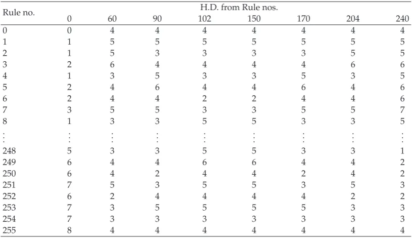
Table 1: H.D.s of three-variable Boolean Functions from linear rules.

Rule no. H.D. from Rule nos.

0 60 90 102 150 170 204 240

0 0 4 4 4 4 4 4 4

1 1 5 5 5 5 5 5 5

2 1 5 3 3 3 3 5 5

3 2 6 4 4 4 4 6 6

4 1 3 5 3 3 5 3 5

5 2 4 6 4 4 6 4 6

6 2 4 4 2 2 4 4 6

7 3 5 5 3 3 5 5 7

8 1 3 3 5 5 3 3 5

..

. ... ... ... ... ... ... ... ...

248 5 3 3 5 5 3 3 1

249 6 4 4 6 6 4 4 2

250 6 4 2 4 4 2 4 2

251 7 5 3 5 5 3 5 3

252 6 2 4 4 4 4 2 2

253 7 3 5 5 5 5 3 3

254 7 3 3 3 3 3 3 3

255 8 4 4 4 4 4 4 4

Cellular AutomatonHCA, for example,135,135,135,135PB is a UCA,0,60,72,72NB is a HCA.

For a UCA, the Boolean function applied to each cell will be called the rule of the CA. So for a UCA, we can obviously drop the superscript “i” from the local mappingfi _and simply denote it asf. for example. for the 4-bit CA230,230,230,230PB, the rule of the CA is Rule 230 and the CA will be called the “Rule 230 CA” of 4 bits with periodic boundary conditions. Henceforth, we will use the following notation UCAnNB, UCAnPB, HCAnNB, and HCAnPB for an n-bit CA. For our purpose, we will be mostly interested in elementary CA defined by Wolfram2to be one-dimensional binary CA with a symmetrical neighborhood of sizep3 for each cell so thatxit1_fi_xi

−1t, xit, xi1t, i2,3, . . . , n−1.

3. Studies on the Hamming Distances between Boolean

Functions and Their Classification

In our paper 5, we proposed and proved a few theorems and their corollaries on the H.D.s between Boolean functions of any number of variables n. Next, we presented a chart of the H.D.s of all the 256 Boolean rules of three variables from the set of the 8 linear rules of three variables and, based on these observations, suggested a classification of three-variable Boolean functions. Here, we have a quick recapitulation.

3.1. Theorems on the H.D.s between Boolean Functions

Theorem 3.1. If the H.D. of an n- variable Boolean function f from another rule g is m, then the H.D.

of the complement of f from the same rule g is (2n₋_m_).

Corollary 3.2. For any nonlinear rule of n variables, there exists at least one aﬃne rule of n variables

(6)

3.2. Classification of Boolean Rules of Three Variables Based on H.D.s from

the Set of Linear Rules

InTable 1, we provide an incomplete chart of the H.D.s of three-variable Boolean functions from the set of linear rules and hence enlist a few interesting observations thereof.

Observations

1H.D. between any two linear rules of 3 variables is 423−1_.

2For any nonlinear rule of 3 variables, there exists at least one linear rule of 3 variables such that the H.D. between the two is smaller than or equal to 4.

3If H.D. of a nonlinear rule of 3 variables from one of the 8 linear rules is evenodd, that from any other linear rule is also even odd; for example, Rules 3 and 255 shown inTable 1.

4If the H.D. of a nonlinear rule of 3 variables from a linear rule of 3 variables is m, say, then the H.D. of the complement of the said nonlinear rule from that linear rule is8−m; for example, Rule 2 and Rule 253.

5If the H.D. of a nonlinear rule of 3 variables from a linear rule of 3 variables is 8, then its H.D. from every other linear rule is 4. There are 8 such nonlinear rules, each of which is, evidently, the complement of one of the 8 linear rules.

6In case the H.D. of a nonlinear rule of 3 variables from a linear rule is even and the said nonlinear rule is not the complement of a linear rule, we have either only one or exactly three linear rules at an H.D. of 2 from the nonlinear rule under consideration. In that case, we have exactly three or only one linear rules, respectively, each at an H.D. of 6 from the nonlinear rule under consideration. The H.D. of the nonlinear rule in question from each of the remaining four linear rules is 4.

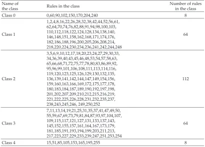
A Boolean rule of 3 variables is said to belong to Class m if m is the minimum possible H.D. of the nonlinear rule from any linear rule of 3 variables, that is, there exists at least one linear rule such that the H.D. of the rule under consideration from this linear rule is m and, if mis the H.D. of the said rule from any other linear rule, thenmis larger than or equal to m. The classification is presented inTable 2.

Comments

1The rules in Class 0 and Class 4 are the aﬃne Boolean functions of 3 variables, Class 0 rules being linear rules and Class 4 rules being the logical complements of the linear rules. The degree of nonlinearity of each of these rules is 0.

2Each rule in Class 3 has its complement in Class 1in the order in which the rules are arranged inTable 3, the ith rule in Class 3 is the complement of the65−ith rule in Class 1,i1,2, . . . ,64; the degree of nonlinearity of each of the Class 1 and Class 3 rules is 1.

(7)

[image:7.600.95.505.112.407.2]

Table 2: Classification of three-variable Boolean rules.

Name of

the class Rules in the class

Number of rules in the class

Class 0 0,60,90,102,150,170,204,240 8

Class 1

1,2,4,8,16,22,26,28,32,38,42,44,52,56,61, 62,64,70,74,76,82,88,91,94,98,100,103, 110,112,118,122,124,128,134,138,140, 146,148,151,158,162,168,171,174,176, 182,186,188,196,200,205,206,208,214, 218,220,224,230,234,236,241,242,244,248

64

Class 2

3,5,6,9,10,12,17,18,20,23,24,27,29,30,33, 34,36,39,40,43,45,46,48,53,54,57,58,63, 65,66,68,71,72,75,77,78,80,83,86,89,92, 95,96,99,101,106,108,111,113,114,116, 119,120,123,125,126,129,130,132,135, 136,139,141,142,144,147,149,154,156, 159,160,163,166,169,172,175,177,178, 180,183,184,187,189,190,192,197,198, 201,202,207,209,210,212,215,216,219, 221,222,225,226,228,231,232,235,237, 238,243,245,246, 249,250,252

112

Class 3

7,11,13,14,19,21,25,31,35,37,41,47,49,50, 55,59,67,69,73,79,81,84,87,93,97,104,107, 109,115,117,121,127,131,133,137,143, 145,152,155,157,161,164,167,173,179, 181,185,191,193,194,199,203,211,213, 217,223,227,229,233,239,247,251,253,254

64

Class 4 15,51,85,105,153,165,195,255 8

Table 3: Classification of three-variable Boolean rules.

27 ₂6 ₂5 ₂4 ₂3 ₂2 ₂1 ₂0

22 0 0 0 1 0 1 1 0

150 1 0 0 1 0 1 1 0

3.3. Subclassification of the Classes of Three-Variable Boolean Rules

Based on Position of Bit- Mismatch with the Nearest Linear Rule

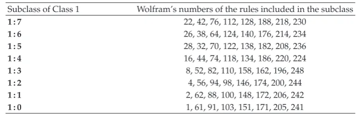
Each Class 1 rule has exactly one linear rule at an H.D. of 1 from itself; that linear rule will be called its nearest linear rule. We express the Wolfram’s number of every Class 1 rule in its 8-bit binary form and compare it with the binary equivalent of the nearest linear rule. If mismatch occurs at bit position 2q_,_q _0,_1,_{2, . . . ,}_{7, the rule is said to belong to Subclass q of Class 1,} denoted by 1 : q; for example, nearest linear rule of Rule 22 is 150 as shown inTable 3.

Therefore, Rule 22 belongs to Subclass 7 of Class 1. Thus, there are 8 subclasses of Class 1, as shown inTable 4.

[image:7.600.97.503.443.483.2]

(8)

[image:8.600.120.476.110.225.2]

Table 4: Subclassification of Class 1 Rules.

Subclass of Class 1 Wolfram’s numbers of the rules included in the subclass

1 : 7 22, 42, 76, 112, 128, 188, 218, 230

1 : 6 26, 38, 64, 124, 140, 176, 214, 234

1 : 5 28, 32, 70, 122, 138, 182, 208, 236

1 : 4 16, 44, 74, 118, 134, 186, 220, 224

1 : 3 8, 52, 82, 110, 158, 162, 196, 248

1 : 2 4, 56, 94, 98, 146, 174, 200, 244

1 : 1 2, 62, 88, 100, 148, 172, 206, 242

[image:8.600.129.475.263.378.2]

1 : 0 1, 61, 91, 103, 151, 171, 205, 241

3 : 7∗ _{233,213,179,143,127,67,37,25}

3 : 6∗ _{229,217,191,131,115,79,41,21}

3 : 5∗ _{227,223,185,133,117,73,47,19}

3 : 4∗ _{239,211,181,137,121,69,35,31}

3 : 3∗ _{247,203,173,145,97,93,59,7}

3 : 2∗ _{251,199,161,157,109,81,55,11}

3 : 1∗ _{253,193,167,155,107,83,49,13}

3 : 0∗ _{254,194,164,152,104,84,50,14}

If the complement of a Class 3 rule belongs to Subclass q of Class 1, then that Class 3 rule is said to belong to Subclassq∗of Class 3, denoted by 3 :q∗. The details are presented in Table 5.

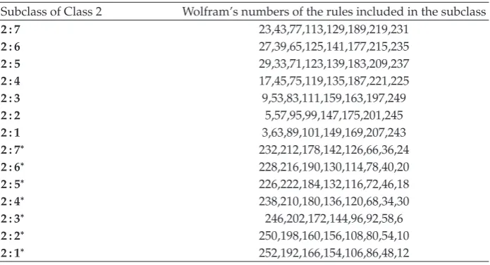
For Class 2 rules, we observe the following.

1Each of the 56 even-numbered rules in Class 2 is the complement of one of the 56 odd-numbered rules in Class 2.

2Every odd rule in Class 2 is at Hamming distance of 2 from exactly one linear rule

and at an H.D. 6 from exactly three linear rules; this single linear rule may be called the nearest linear rule of the odd-numbered rule concerned; naturally, each even rule in Class 2 is at an H.D. of 2 from exactly three linear rules and at an H.D. of 6 from exactly one linear rule, and, hence, for an even Class 2 rule, the nearest linear rule is not unique, for example, rule 6Table 2.

3As a linear rule is necessarily even numbered, the binary representation of any odd rule in Class 2 will definitely diﬀer from that of its nearest linear rule at the bit position 20 _{i.e., at the LSB}_{which is always 1 for an odd rule and 0 for an even}

rule. The bit position of the second mismatch will naturally not be the same for all odd-numbered rules.

(9)

[image:9.600.127.475.111.299.2]

2 : 7 23,43,77,113,129,189,219,231

2 : 6 27,39,65,125,141,177,215,235

2 : 5 29,33,71,123,139,183,209,237

2 : 4 17,45,75,119,135,187,221,225

2 : 3 9,53,83,111,159,163,197,249

2 : 2 5,57,95,99,147,175,201,245

2 : 1 3,63,89,101,149,169,207,243

2 : 7∗ _{232,212,178,142,126,66,36,24}

2 : 6∗ _{228,216,190,130,114,78,40,20}

2 : 5∗ _{226,222,184,132,116,72,46,18}

2 : 4∗ _{238,210,180,136,120,68,34,30}

2 : 3∗ _{246,202,172,144,96,92,58,6}

2 : 2∗ _{250,198,160,156,108,80,54,10}

2 : 1∗ _{252,192,166,154,106,86,48,12}

The nearest linear rule of Rule 3 is 0. Therefore, Rule 3 belongs to Subclass 1 of Class 2, denoted by 2 : 1 and complement of Rule 3255−3252. Thus, Rule 252 belongs to Subclass 1∗of Class 2, denoted by 2 : 1∗as shown inTable 6.

4. Characterization of Nonlinear UCA STDs in Terms of

Deviation from Linearity

4.1. The State Transition Diagram of a UCA

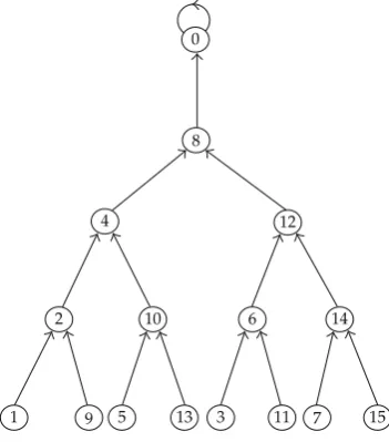
The evolution of a CA can be completely described by a diagram in which each state is connected to its successor by a properly directed line segment. This diagram is called the State Transition Diagram abbreviated as STD of the CA. In other words, the STD of a CA is essentially a directed graph where each node represents one of the states of the CA and the

edges signify transitions from one state to another. The STD of the UCA Rule 170 NB is shown

inFigure 1.

As already mentioned the structure of a linear CA STD is very well behaved and has been exhaustively studied. But, unfortunately, even for a moderate number of input variables, the linear rules constitute practically a microscopic fraction of the great multitude of Boolean functions. The nonlinear rules are, however, at various degrees of nonlinearity. So the idea that those nonlinear rules that are not so distant from linear rules may be studied in terms of their similarityor, equivalently, dissimilaritywith their closest linear rules appears quite appealing and viable, and we have tried to work on it.

(10)

[image:10.600.124.476.111.227.2]

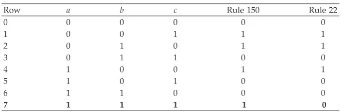
Table 7: Comparison of Truth Tables of Rules 150 and 22.

Row a b c Rule 150 Rule 22

0 0 0 0 0 0

1 0 0 1 1 1

2 0 1 0 1 1

3 0 1 1 0 0

4 1 0 0 1 1

5 1 0 1 0 0

6 1 1 0 0 0

7 1 1 1 1 0

As such, the new ruleoﬀspringobtained from another ruleparentis called a mutant of the latter. Thus, in our classification, Class 1 rules may be regarded as one-bit mutants of linear rules, Class 2 rules as two-bit mutants of linear, rules and so on. Of these, the one-bit mutants are of utmost importance because, quite understandably, they can be expected to exhibit a greater similarity with linear rules than any other rule. This is found to be true in practice, as will be elaborated in the subsequent sections.

4.2. The Concept of Deviant States

If we compare the STD of a UCA with a Class 1 nonlinear rule all subclassesor an odd-numbered nonlinear rule from Class 2 with that of a same-sized UCA with its nearest linear rule, we observe that a considerable number of states have identical successors in both the STDs while the successors of other states diﬀer in the two STDs. For a given sizenof CA, we define a state of a nonlinear UCA, to which a Class 1 rule or an odd Class 2 rule has been applied, as a deviant state for that nonlinear rule if the successor of the state under consideration in the S.T.D. of the nonlinear UCA taken is diﬀerent from its successor in the STD of the nearest linear rule UCAof the same size. For example, Rule 128 belongs to Class 1 : 7 and its nearest linear rule is 240. Comparison of their STDs for a UCA4NB reveals that only the states 7, 14,

15 have diﬀerent successors in the two STDs, so for Rule 128 UCA4NB, the deviant states are

7, 14, 15.

It is evident from this discussion that the deviant states have been defined with respect to the nearest linear rule onlyand not just any linear rulebecause we can expect maximum similarity of the STD of a nonlinear rule with the STD of its nearest linear rule. For this same reason, deviant states have been defined for the above subclasses only; for other subclasses, the nearest linear rule is not uniquely defined.

4.3. An Algorithm for Deducing the Set of Deviant States

For a Class 1 rule, the deviant states for a given size of CA can be easily determined and, hence, the STD of such a nonlinear rule, say f, can be easily deduced from that of its nearest linear rulefLbyAlgorithm 1.

Illustration

(11)

1 2

0

3 4

5

6

7 8

9 10

11 12

13

14

[image:11.600.211.387.99.299.2]

15

Figure 1: S.T.D. of170,170,170,170NB.

Table 8: Determination of deviant states and their successors for Rule 22 UCA4NB.

Deviant states Successor in Rule 150 UCA4NB Successor in Rule 22 UCA4NB

Binary Decimal Decimal Binary Decimal Binary

0 1 1 1 7 10 1 0 1 0 1 0 0 0 8

1 1 1 0 14 5 0 1 0 1 0 0 0 1 1

1 11 1 15 6 0 11 0 0 00 0 0

the STD of22,22,22,22NB from that of150,150,150,150NB are shown with the help of Tables7and8and Figures2and3.

4.4. Comments on Deviant States

1Since the sequence to be searched may occur more than once in the same state and, in case of multiple occurrences, the repeating sequences may or may not overlap, it is clear that the task of identifying the deviant states and deducing their successors by the bit-toggling method becomes increasingly diﬃcult with increasing length of CA.

2Determination of the deviant states for odd Class 2 rules can be similarly accomplished by first locating the two positions of bit-mismatch and then searching for at least one of the two corresponding 3-bit combinations in the CA state. We could also proceed in two steps by considering one mismatch at a time. Obviously, the task is more diﬃcult than that for the Class 1 case.

3The set of deviant states for a given f depends strongly on the number of bits in the CA as well as on the boundary conditions null/periodic; for example, for 22,22,22,22NB, the set of deviant states is {7,14,15} whereas that for

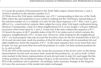
[image:11.600.96.506.355.420.2]

(12)

1Locate the position of bit-mismatch in the Truth Table output column betweenfandfL

which is identical to the subclass number off.

[image:12.600.105.493.76.337.2]

2Write down the 3-bit input combination, saya∗b∗c∗corresponding to that row of the Truth

Table where the said mismatch occurswhich is nothing but the 3-bit binary representation of

the subclass number off; evidently, it is only for this input sequencea∗b∗c∗thatfandfLgive

diﬀerenti.e., complementaryoutputs, their output for every other 3-bit input combination being

identical. Consequently, a state of a three-neighborhood UCA of any length n will give diﬀerent

successors when acted upon byfandfLif and only if the state contains the sequencea∗b∗c∗.

3Search the space of all 2n_{possible states of the UCA for states each of which contains the}

sequenceneighborhooda∗b∗c∗at least once. However, while looking for the neighborhood,

a∗b∗c∗ we must properly take into account the boundary values for the two terminal bits of the CA.

4In each deviant state, mark the position of that bit which, along with its immediate left and

right neighbours, forms the sequencea∗b∗c∗. As the same sequence may occur more than once

in state, we may get more than one such bit-positions in a state. Let these marked positions be

þ1,þ2and so forth.

5In the STD of the nearest linear rule, locate the successors of the deviant states; in the binary

representation of each such successor state, mark the bit-positionsþ1,þ2and so forth.which

were marked in the binary representation of each deviant state in step4and toggle the bits

at these positions; the resulting bit string will give us the successor of the deviant state in the STD of the nonlinear rule in question. Accordingly, make necessary changes in the diagram.

6Leave the successors of the nondeviant states unchanged.

Algorithm 1

4For given CA length and boundary conditions, all the rules in a subclass have identical deviant states because bit-mismatch with the respective nearest linear rules occurs at the same bit-position but the set of deviant states, in general, varies from one subclass to another.

5For the periodic boundary case, the bits in any state may be supposed to be arranged in a ring or circle so that it is somewhat less diﬃcult to identify the deviant states because such states will occur in rotationally equivalent sets7; for example, for22,22,22,22PB,7₁₀ ≡0111₂is clearly a deviant state and14₁₀ ≡1110₂,

13₁₀ ≡ 1101₂, 11₁₀ ≡ 1011₂ are rotationally equivalent to 7, so we can immediately declare them deviant states. It is also interesting to note that it is suﬃcient to deduce the successor of any one state from this set by the bit-toggling method because their successors are also rotationally equivalent and hence occupy equivalent positions in the STD.

4.5. The Significance of the Proportion of Deviant States in an STD

Let us define a quantity Pds, called the proportion of deviant states for an n-bit nonlinear UCA, asPdsNds/2n_{, where}_Nds_{number of deviant states of the UCA considered and 2}n is the total number of states of the UCA.

The rationale underlying the introduction of the concept of deviant states is that the behavior of the deviant states embodies the eﬀect of the bit-mismatchesbetween f andfL

(13)

1 2

0 3

4

5

6

7

8

9

10

11

12 13

14

[image:13.600.236.367.97.224.2]

15

Figure 2: STD of150,150,150,150NB.

linear rule until and unless a deviant state is encountered; when a deviant state is actually reached, the evolution deviates from the linear path, reaches some state, and henceforward resumes the linear path till the next deviant state is reached. As such, the proportion of deviant

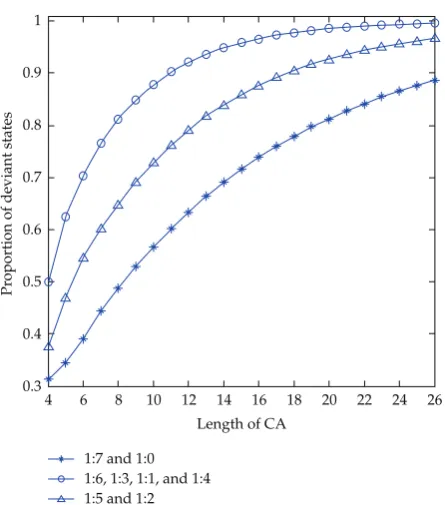
states in a CA may provide us with some measure of the deviation from linearity of a nonlinear rule with respect to CA state transitions. This discussion reveals that it is not just the number of bit-mismatchesi.e., degree of nonlinearitybut also the actual positions of bit-mismatch, which determine how much a nonlinear UCA STD diﬀers both qualitatively and quantitatively from the closest linear STD. With this in mind, we investigated the dependence ofPdson the length of the CA for all Class 1 subclasses for the periodic boundaryPBcase, and the results are presented inTable 9andFigure 4.

Comments on

Figure 4

1For any given length of CAPB,Pds1 : 7 Pds1 : 0as the neighborhoods 111 and

000 exhibit complementary symmetry7,Pds1 : 5 Pds1 : 2as the neighborhoods

101 and 010 also exhibit complementary symmetry,Pds1 : 6 Pds1 : 3 Pds1 : 4

Pds1 : 1as the neighborhoods 110 and 011 exhibit reflection symmetry7, 011 and

100 show complementary symmetry, and 100 and 001 show reflection symmetry again.

2As the length of CA PB increases, the proportion of deviant states, say Pds, tends towards unity for any subclass of Class 1, which means that the eﬀect of nonlinearity becomes more pronounced but following inequality is always maintained:Pds1 : 7,1 : 0 < Pds1 : 5,1 : 2 < Pds1 : 6,1 : 3,1 : 4,1 : 1 with the diﬀerence between the last two becoming significantly smaller than that between the first two.

5. Conclusion and Future Research Directions

In this paper, we have identified a group of elementary nonlinear uniform cellular automata

(14)

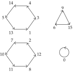
0 1

2 3

4 5

6

7 8

9

10 11

12 13

14

[image:14.600.227.370.100.223.2]

15

Figure 3: STD of22,22,22,22NB.

0.3 0.4 0.5 0.6 0.7 0.8 0.9 1

4 6 8 10 12 14 16 18 20 22 24 26

Length of CA

Pr

oportion

of

deviant

states

1:7 and 1:0 1:6, 1:3, 1:1, and 1:4 1:5 and 1:2

Figure 4: Plot of proportion of deviant states versus length of CAperiodic boundfor various subclasses

of Class 1.

the linear rules. As such, it would apparently be wiser to classify Boolean functions on the basis of distance from the set of aﬃne rulesi.e., degree of nonlinearityrather than the set of linear rules and, in that case, the entire set of aﬃne ruleslinear rules and their complements must be taken as the standard. We are exploring this possibility. Although the idea is still in an incipient state, it appears quite promising.

Another of our current eﬀorts is aimed at deducing a possible formula for the number of deviant states in terms of the length n of the CA for a given nonlinear rule and given boundary conditions.

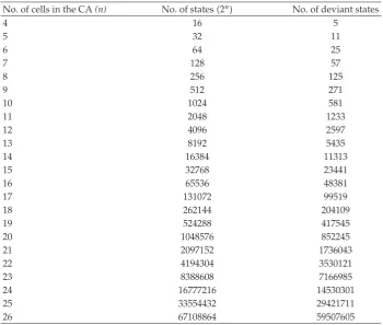
[image:14.600.189.412.266.519.2]

(15)

[image:15.600.125.476.113.410.2]

Table 9: Table showing the variation in the number of deviant states for a 1 : 7 rule with CA length.

No. of cells in the CA (n) No. of states2n _{No. of deviant states}

4 16 5

5 32 11

6 64 25

7 128 57

8 256 125

9 512 271

10 1024 581

11 2048 1233

12 4096 2597

13 8192 5435

14 16384 11313

15 32768 23441

16 65536 48381

17 131072 99519

18 262144 204109

19 524288 417545

20 1048576 852245

21 2097152 1736043

22 4194304 3530121

23 8388608 7166985

24 16777216 14530301

25 33554432 29421711

26 67108864 59507605

the study presented in this paper, it appears that even if the neighborhood sizenumber of independent variablesincreases, we can still possibly isolate a set of mutants of linear rules, which can be characterized in terms of deviant states. It is germane to mention here that, as already pointed out in7, one-bit mutation amounts to1/23_×₁₀₀_%_{12.5% change for a}

3-variable function, to1/25_×₁₀₀_%_{3.125% for a 5-variable function, and so on. In other}

words, the eﬀect of mutation of a CA rule on a CA evolutionand thus the deviation of the CA STD from linearitydecreases as the size of the neighborhood increases. So, for a given length of CA and a given nonlinear rule, the proportion of deviant states must decrease with increasing size of neighborhood.

References

1 J. von Neumann, The Theory of Self-Reproducing Automata, A. W. Burks, Ed., Univ. of Illinois Press,

Urbana, Ill, USA, 1966.

2 S. Wolfram, Ed., Theory and Applications of Cellular Automata, vol. 1 of Advanced Series on Complex

Systems, World Scientific, Singapore, 1986.

3 S. Wolfram, A New Kind of Science, Wolfram Media, Champaign, Ill, USA, 2002.

4 I. Wegener, The Complexity of Boolean Functions, Wiley-Teubner Series in Computer Science, John Wiley

& Sons, Chichester, UK, 1987.

5 P. P. Choudhury, S. Sahoo, M. Chakraborty, S. K. Bhandari, and A. Pal, “Investigation of the global

(16)

6 S. Sahoo, P. P. Choudhury, M. Chakraborty, and B. K. Nayak, “Characterization of any non-linear Boolean function using a set of linear operators,” Journal of Orissa Mathematical Society, vol. 29, no. 1-2, pp. 111–133, 2010.

7 A. Wuensche and M. Lesser, The Global Dynamics of Cellular Automata, An Atlas of Basin of Attraction

Fields of One-Dimensional Cellular Automata, vol. 1 of Santa Fe Institute Studies in the Sciences of Complexity, Addison Wesley, 1992.

8 C. Moore, “Predicting nonlinear cellular automata quickly by decomposing them into linear ones,”

Physica D, vol. 111, no. 1–4, pp. 27–41, 1998.

9 S. Takakaju, “Non-linear cellular automata with group structure,” IEIC Technical Report, vol. 99, no.

33, pp. 37–44, 1999.

10 R. Smolensky, “Algebraic methods in the theory of lower bounds for boolean circuit complexity,” in

Proceedings of the Annual ACM Symposium on Theory of Computing, pp. 77–82, 1987.

11 B. H. Voorhees, Computational Analysis of One-Dimensional Cellular Automata, vol. 15 of World Scientific

Series on Nonlinear Science. Series A: Monographs and Treatises, World Scientific, River Edge, NJ, USA,

1996.

12 B. Voorhees, “Predecessors of cellular automata states. II. Pre-images of finite sequences,” Physica D,

(17)

Submit your manuscripts at

http://www.hindawi.com

Hindawi Publishing Corporation

http://www.hindawi.com Volume 2014

Mathematics

Journal of

Hindawi Publishing Corporation http://www.hindawi.com

Differential Equations

International Journal of

Volume 2014

Applied MathematicsJournal of

Mathematical PhysicsAdvances in

Complex Analysis

Journal of

Optimization

Journal of

Combinatorics

http://www.hindawi.com Volume 2014 International Journal of

Journal of

Function Spaces

Abstract and Applied Analysis

International Journal of Mathematics and Mathematical Sciences

Hindawi Publishing Corporation http://www.hindawi.com Volume 2014

The Scientific

World Journal

Discrete Dynamics in Nature and Society

http://www.hindawi.com Volume 2014 Hindawi Publishing Corporation

Discrete Mathematics

Journal of

Characterization of the Evolution of Nonlinear Uniform Cellular Automata in the Light of Deviant States

Research Article