Munich Personal RePEc Archive
Endogenous selection of aspiring and
rational rules in coordination games
Dziubinski, Marcin and Roy, Jaideep
Lancaster Uniersity, Brunel University
25 November 2007
Endogenous Selection of Aspiring and Rational
rules in Coordination Games
Marcin Dziubi´nski Department of Economics,
Lancaster University,
Lancaster LA1 4YW, United Kingdom. [email protected]
Jaideep Roy
Department of Economics, School of Social science,
Brunel University,
Uxbridge, Middlesex UB8 3PH, United Kingdom. [email protected],
Tel: +44 (0) 18952 65539
February 2007
Abstract
The paper studies an evolutionary model where players from a given population are randomly matched in pairs each period to play a co-ordination game. At each instant, a player can choose to adopt one of the two possible behavior rules, called therational rule and the as-piring rule, and then take actions prescribed by the chosen rule. The choice between the two rules depends upon their relative performance in the immediate past. We show that there are two stable long run outcomes where either the rational rule becomes extinct and all play-ers in the population achieve full efficiency, or that both the behavior rules co-exist and there is only a partial use of efficient strategies in the population. These findings support the use of the aspiration driven behavior in several existing studies and also help us take a comparative evolutionary look at the two rules in retrospect.
Keywords: Co-evolution, Aspirations, Best-response, Random matching, Coordination games.
1
Introduction
It is well accepted today that models of rational behavior do not fare well in many experiments. This is perhaps because in relatively complex environ-ments, expected payoff maximization requires either too much knowledge about the environment or that the available information is hard to analyze. Moreover, it is at times extremely difficult to gather information required to form reasonable beliefs regarding the nature of the opponents with whom a player plays a game. If one is allowed to assume that in face of such complexities, rational behavior entails a cost of implementation, it is not surprising why many of us at times may prefer to use more simple behavior rules.
Various researchers have assumed alternative behavior rules, which are simple and where players do not necessarily use best responses when deciding about their strategies. One such approach that has gained much popularity is the so called reinforcement or stimulus learning behavior. This approach assumes that a player takes actions which are relatively more successful and discard those which are not. A celebrated behavior rule that describes such reinforcement methods is the one driven by payoff aspirations. According to this rule, a player has a payoff aspiration and takes an action. If the current action meets his payoff aspiration, he continues with it while if he is disappointed (because it fails to meet his current aspiration), he experi-ments with other available actions. There are many outstanding studies of evolution of play where players are assumed to be aspiration driven (for an excellent survey, see Bendor et al. [2001]; also see the section on literature review below). All of the existing papers assume that all players involved in the studied environments are aspiration driven. Given this, the present pa-per asks the following question: are naive behavior rules, like the one based on aspirations, strong enough to survive evolutionary pressures from more efficient rules like that of expected payoff maximization if implementing such efficient rules is not too costly?
no matter how small.1 On the other hand, those who adopt the aspiring
rule give up this search for costly information about their opponents and simply adopt a population wide fixed aspiration and take actions to check if the action taken meets this adopted aspiration. Thus at any instant of time, the population can be divided into two groups, those who are currently following the rational rule and those who are currently aspiring. We assume that the difference of the average performances of these two groups of players is publicly available. If at any instant, the average performance of one group exceeds that of the other, then there is some (but not necessarily full) flow of players from the low performing group into the more successful one. Time is continuous and this process is left to go on for ever. This environment gives rise to a two-dimensional dynamic system where we keep track of the fraction of aspiring players in the population and the fraction of aspiring players who play the efficient equilibrium strategy. It turns out that we are also able to report on what rational players do. We show that the limit behavior of our system depends crucially on whether the social aspiration level is high or low. In case of a high social aspiration, there are only two stable rest points of the system: the first where the rational rule gets extinct and all players follow the aspiring rule and play the efficient equilibrium strategy, and the second where both rules survive but all players who use the rational rule play the inefficient equilibrium strategy while those who use the aspiring rule have a positive fraction who play the efficient equilibrium strategy. Unlike in the case with high aspirations, we show that with a low social aspiration, there is no chance of a stable mixed population – the rational rule gets extinct independent of the intial conditions.
1.1 Related Literature
Models where players use reinforcement learning rules first appear in the mathematical psychology literature with studies by Estes [1954], Bush et al. [1954], Bush and Mosteller [1955] and Suppes and Atkinson [1960]. The com-puter science and engineering literature has also used such models represent-ing various natures of automata learnrepresent-ing as in Lakshmivarahan [1981], Naren-dra and Mars [1983], NarenNaren-dra and Thathachar [1989] and Papavassilopoulos [1989].
This area in economics was pioneered by Simon [1955, 1957, 1959], Cross [1973] and Nelson and Winter [1982]. The focus since then has been on
re-1
peated games (and in particular the repetition of the Prisoners’ Dilemma) and most models typically show that players learn to coordinate on effi-cient outcomes, which may not (or may) be strategic equilibrium points [see for example, Bendor et al. [1994], Karandikar et al. [1998], Kim [1995] and Pazgal [1995]]. Limited work with aspiration driven rules has been done with a large population of players who are matched in pairs to play 2×2 games. Two most important works in this area are by Dixon [2000] and Palomino and Vega-Redondo [1999]. Dixon’s framework assumes that a continuum of players are once and for all matched in pairs to form stable partnerships and play bilateral games (including the Prisoners’ Dilemma or the Cournot market games). In his setup, individual players form aspira-tions from some statistic that signals the performance of players in other pairs (or markets). He shows that play in each pair converges to joint payoff maximization regardless of initial conditions. Palomino and Vega-Redondo consider a non-repeated setting where the Prisoners’ Dilemma is played by randomly matched aspiring players with matchings taking place indepen-dently at each instant of time (and hence their approach is evolutionary rather than repeated and in this sense their work is closest to ours). In their setting, aspiration of each player depends on the payoff experiences of the entire population (and this dependence is symmetric across all players rendering a common aspiration for each of them) and that this social aspi-ration evolves over time. In our case as well, the aspiaspi-ration level is modeled as a social attribute though it remains fixed over time. They show that in the long run a positive (but less than 1) fraction of the population are able to cooperate. In view of Palomino and Vega-Redondo, Dixon’s work shows that stability of partnership is essential for full efficiency in the long run.
whom) each player interacts.2 Binmore and Samuelson [1997] study
endoge-nous learning rules in a global setting, as in ours. They view the evolutions of actions, guided by a particular learning rule, as a process that proceeds at a speed which is rapid compared to the evolution of the learning rule itself. In some sense though, in their model players use a learning rule forever and then evaluate what they obtain in this first round of infinite regress – called the long run, and then adopt a new rule and this process goes on for infinite rounds of these infinite regresses – called the ultra long run. Also, they identify a learning rule with the aspiration level which it incorporates. In our view, this is essentially a single learning rule, the aspiring rule, but with a very slow and experimental aspiration updating mechanism. Nevertheless, they show that this double infinity regress leads to the selection of the risk dominant equilibrium. This in itself is a very important result.
The rest of the paper is structured as follows. In the following section we describe in details the model. The results are stated and proved in section 3 with some proofs moved to an appendix to maintain a smooth exposition. In section 4 we report some simulated trajectories of our dynamic system to support some finer points of our analysis. The paper concludes in section 5.
2
The model
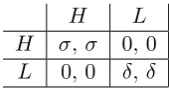
Consider a fixed set of individuals (or players) Ω with the cardinality of the continuum. At each time t ∈ [0,∞) individuals in Ω are randomly matched in pairs to play a coordination game presented in the figure 1, where 0< δ < σ.
H L
H σ,σ 0, 0
[image:6.595.254.339.478.526.2]L 0, 0 δ,δ
Figure 1: Coordination game
At any instant of time t, the set Ω consists of two distinct sets, the set of rational players R, and the set of aspiration driven players A. We use
a to denote the fraction (with respect to Ω) of aspiration driven players in the population andµto denote the fraction (with respect toA) of aspiration driven players playingH.
Aspiration driven players use either the pure strategy H or the pure strategyL– the exact behavioral assumptions are stated later in this section. We assume that rational players are myopic and always play pure strategy
2
best responses. Let p ∈ [0,1] be the probability belief held by a generic rational player for the event that in case his opponent is also a rational player then his opponent will play the pure strategy H. Hence, the probability beliefs held by a generic rational player that his opponent (who could either be a rational player or an aspiring player) will play pure strategies H and
L,respectively, are Pr(H) =aµ+ (1−a)p and Pr(L) = 1−Pr(H). Given
a, µand p, the expected payoff of a generic rational player from playingH
and L,respectively, are
Er(H;a, µ, p) = σ[aµ+ (1−a)p], and
Er(L;a, µ, p) = δ[1−(aµ+ (1−a)p)] .
Hence this generic rational player playsH with probability 1 whenever
σ[aµ+ (1−a)p] ≥ δ[1−(aµ+ (1−a)p)] , that is
aµ+p(1−a) ≥ δ σ+δ.
Since the above inequality is true for any p ∈ [0,1], we can conclude that if aµ ≥ δ
σ+δ, then the above inequality is satisfied. Similarly, it is easy
to see that if aµ ≤ a− σ
σ+δ, then the reverse of the above inequality is
satisfied and this generic rational player playsLwith probability 1. Hence, given the game, in the region of (a−µ) plane where aµ ≥ δ
σ+δ, a generic
rational player always plays H while in the region of (a−µ) plane where
aµ≤a−σσ+δ, this generic rational player always playsL, independent of the belief probability p. Now let us concentrate on the remaining region of the (a−µ) plane witha−σ/(δ+σ)< aµ < δ/(σ+δ) where beliefs about what “other” rational players play do matter in deciding upon a generic rational best response. Given a, µ and p, we impose symmetry across all rational strategies. Hence, p is to be interpreted as the probability with which all rational players playH. Given this, the expected payoff of a generic rational player is given by
Er(p;a, µ, p) =σ(aµ+ (1−a)p)p+δ(a(1−µ) + (1−a)(1−p))(1−p).
It is easy to check that for any value ofp,
Er(p;a, µ, p)≤max{σ(1−a(1−µ)), δ(1−aµ)}.
On the other hand, notice that
Er(p;a, µ, p) =
σ(1−a(1−µ)) ifp= 1, δ(1−aµ) ifp= 0.
mean that all rational players playH with probability 1 ifσ(1−a(1−µ))≥
δ(1−aµ) and otherwise playLwith probability 1. Notice that whenever the conditionaµ≥ σ+δδis satisfied, so is the conditionσ(1−a(1−µ))≥δ(1−aµ). Similarly, whenever the conditionaµ≤a− σ
σ+δ is satisfied, so is the condition
σ(1−a(1−µ))≤δ(1−aµ).
Choosing between these rational best responses requires on part of any rational player to constantly update his information regarding the values of
a and µ. We assume that acquiring this information is costly, no matter how small, and we denote this cost that each rational player has to incur as
̺∈(0, δ).
During the whole process each player can change his behavior rule, that is either adopt the rational rule described above or adopt the aspiring one which we shall soon describe. This choice depends on the difference between average payoffs of the particular types of players and the exact procedure for this change is provided below. For the moment, notice that if̺= 0,the average payoff of rational players, by the very definition of rationality, can never be less than the average payoff of aspiration driven players.
As the values ofaandµevolve, rational players switch between strategies
H and L, depending on which of them is currently a best reply (as defined above). We assume that this switching process is not instantaneous – the whole rational population does not switch at once, but that there is a fraction of rationals that do so while the remaining are “about to do so”. This is motivated by the fact that current actions and rules have an inertia, no matter how small and to capture this notion of inertia, we incorporate a strictly increasing and continuously differentiable function ξ(a, µ) on the interval [−ε, ε], representing the probability with which a rational player plays H,such that
ξ(a, µ)
= 0 ifEr(1;a, µ,1)−Er(0;a, µ,0)≤ −ε,
∈(0,1) if −ε <Er(1;a, µ,1)−Er(0;a, µ,0)< ε,
= 1 ifEr(1;a, ν,1)−Er(0;a, µ,0)≥ε.
(1)
Here ε > 0 reflects the size of the area in which the rational population is in a switching phase.3 In the remaining part of the paper we will write ξ
instead ofξ(a, µ) for convenience.
As mentioned above, the change of players’ behavior rules depends on the difference between the average payoffs of populations different types. So, given a, µ and ξ, the average payoff πa of the aspiration driven population
3
at any instant is given by
πa(µ, a) =σµ(aµ+ (1−a)ξ) +δ(1−µ)(a(1−µ) + (1−a)(1−ξ)), (2)
while theaverage payoff πr of the rational population at any instant is given
by
πr(µ, a) =σξ(aµ+ (1−a)ξ) +δ(1−ξ)(a(1−µ) + (1−a)(1−ξ))−̺. (3)
We assume that the differenceπa(µ, a)−πr(µ, a) is publicly observed. The
probability rate at which a player changes his type is modelled by use of a strictly increasing (on [0,+∞)) and continuously differentiable function
g(ψ) satisfying
g(ψ)
= 0 ifψ≤0,
>0 ifψ >0. (4)
From the above assumptions it follows thatg′
(ψ) = 0 forψ≤0. Given this functiong(·), the change in time of the fraction of aspiration driven players is given by
˙
a=A(a, µ) =κ1
−g(−ψ(a, µ))a
+g(ψ(a, µ))(1−a)
, (5)
whereκ1 >0 is some arbitrary speed adjustment parameter andψ(a, µ) = πa(µ, a)−πr(µ, a).
We are now in a position to describe the behavioral assumptions on the aspiring rule. A player who has decided to follow the aspiring rule essentially sets a payoff aspiration equal to a given (and fixed over time) aspiration level which is common to all players in the aspiring population. We denote this
social aspiration level as α. With this payoff aspiration, a player who is currently following the aspiring rule takes an action, which in our game is either H or L, and receives an individual payoff of π ∈ {0, δ, σ}. This social aspirationαand the realization of his current payoffπ gives rise to an individual dissatisfaction level of χ=α−π. The probability rate at which an aspiration driven player with dissatisfaction level χ, who still wishes to follow the aspiring rule, changes his current strategy is given by a strictly increasing (on [0,+∞)), continuously differentiable functionf(χ) satisfying
f(χ)
= 0 ifχ≤0,
>0 ifχ >0 (6) which captures the notion that if an aspiring player is satisfied with his current payoff (that isχ≤0), and if he decides to remain an aspiring player in the next instant, then he sticks to his current action in the next instant; otherwise, if he still wants to remain an aspiring player, he experiments with the other available action with a positive probability.4
4
Given the probability rate f, we can now describe the change in time of the fraction µ of aspiration driven players playing H. In doing so the following observations/assumptions are made:
• There are three factors that affectµ, (i) the switch of actions amongst current aspiration driven players who choose to remain aspiration driven, (ii) the mass of current aspiration driven players who chose to become rational and (iii) the mass of currently rational players who choose to become aspiring.5
• In case of (i), this is entirely determined by the functionf.
• We assume that those aspiring players who leave the aspiring popula-tion are uniformly distributed over the two available current acpopula-tions
H and L.
• We assume that those rational players who join the aspiring population become aspiration driven and start out by playingH with probability
µ.
In our settings it is reasonable to consider 0< α≤σ which we assume henceforth. The above observations and assumptions lead us to the following expression for ˙µgiven by
˙
µ=M(a, µ) =κ2
−f(α)µ(a(1−µ) + (1−a)(1−ξ)) +f(α)(1−µ)(aµ+ (1−a)ξ)
+f(α−δ)(1−µ)(a(1−µ) + (1−a)(1−ξ)).
, (7)
whereκ2 >0 is some arbitrary speed adjustment.
Remark 1. There is one important remark that must be made about our model. It can be used only ifa6= 0, since calling µ a fraction of aspiration driven players is not valid otherwise. However, as we shall see in the next section, the dynamic system described by the above differential equations (5) and (7) never reaches a state where a = 0, when started from any state wherea6= 0. Thus we can draw valid conclusions about the phenomenon we study using the above proposed model.
In this paper we study the two-dimensional dynamic system in the (a−µ) plane characterized by the two equations of motion (5) and (7). Our goal is to find stable rest points of this system and identify their basins of attraction. This analysis is done in the following section.
5
Given our functiong(·), there can be no two-way flow in our model. Hence, at any
3
The analysis
The area under consideration is Z = [0,1]×[0,1], with (a, µ) ∈ Z. The behavior of rational players gives rise to a partition ofZ into two areas, one where rationals playH while the other where they play L. Let
s(a, µ) =σ(1−a(1−µ))−δ(1−aµ),
and first define the regions
MH = {(a, µ) : (a, µ)∈M and s(a, µ)>0}, ML = {(a, µ) : (a, µ)∈M and s(a, µ)<0}
and their subsets respectively as
H = {(a, µ) : (a, µ)∈Z and aµ > δ/(δ+σ)}and
L = {(a, µ) : (a, µ)∈Z and aµ < a−σ/(δ+σ)}.
Notice that H ⊂ MH, L ⊂ ML, MH ∩ ML = ∅ and MH ∪ ML = Z. Morover while in MH, all players using the rational rule play H. Simi-larly while inML, all players using the rational rule play L. All the areas discussed above are represented in figure 2.
Since in the neighborhood of the lines(a, µ) = 0,rational players switch between strategies, so it will be called the switch line. The area Sε =
{(a, µ)∈ Z : −ε≤s(a, µ)≤ε, ε >0} where, as exemplified in (1), rational switching takes place will be called theswitch area of sizeε. We will assume that ε is as small as possible and drop the subscript ε and denote this switching area as S. Since ε is arbitrarily small, we will ignore analysis withing this area.
Let v : Z → R2 be the vector field defined by (5) and (7). Since v
is continously differentiable on R2 and Z is closed and bounded, so v is
Lipschitz.6 Notice that since v does not point outward on the boundary of
Z, so any trajectory starting from Z remains in Z. Moreover, since v is Lipschitz, there exists a unique solutionφv(t,x0) of the system of differential
equations (5), (7) for any initial condition x0 ∈ Z. Notice also that any
trajectory starting from initial condition (0,0) remains on the line a = 0 until µ > (σ−̺)/σ. Moreover µ > (σ −̺)/σ implies ˙a > 0 and µ = 0 implies ˙µ >0. These observations, together with the uniqueness of solutions and the fact that our system is autonomous guarantee that every trajectory starting from initial conditions (a, µ) where a∈(0,1] never reaches a state wherea= 0. This justifies remark 1.
Our analysis will be divided into two cases – when the social aspiration level is high, that is δ < α ≤σ, and when it is low, that is 0< α ≤δ. In both cases we will analyse the areasMH andML separately.
6
1 0
1
a
µ
σ δδ+
σ δ
δ
+
σ δ σ−
σ δ
σ
+
MH
ML
L
[image:12.595.164.431.128.409.2]H
Figure 2: Areas of different rational best responses.
3.1 High aspiration level
Throughout this section we will assume that the aspiration level is high, that is δ < α≤σ.
3.1.1 The analysis with an initial condition in MH
In this section we will study the behavior of the system with initial conditions in the regionMH where all rationals playH. Our main result for this case is as follows
Main Result 1. Consider any coordination game such that0< δ < σ and an aspiration level α ∈(δ, σ]. Let X = [0,1]×[δ/(δ+σ) +ε,1]⊃ H − S,
x∈ X and let φv(t,x) be a solution of the system of differential equations
(5), (7). Thenlimt→+∞φv(t,x) = (1,1).
Remark 3. It is also important to note that the result is independent of the value of ̺, provided that ̺ ∈(0, δ). Thus no matter how small ̺ is, as long as it is positive, the system starting inX will converge to the restpoint
(1,1).
If the system starts in the areaMH ⊂ Z, then the expressions forψand
M have the following form:
ψ(a, µ) = ψH(a, µ) =a(1−µ)2(δ+σ)−(1−µ)σ+̺, (8)
M(a, µ) = MH(a, µ) =κ2(f(α−δ)a(1−µ)2+f(α)(1−a)(1−µ)).(9)
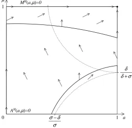
The phase plane diagram for this situation is presented in figure 3 below.
1 0
1
a
µ
σ δ
δ
+
σ δ σ− AH(a,µ)=0
[image:13.595.161.431.301.563.2]MH(a,µ)=0
Figure 3: Phase plane diagram when all rationals playH.
The following lemma shows that if all rational players play H, there is only one rest point inZ which is asymptotically stable7 by proving that the
rest point is ageneric saddle node (see [Hubbard and West, 1991, part II, p. 281] or theorem 2 in the appendix for the characterisation of generic saddle nodes).
7
Lemma 1. Suppose the system begins in MH. Then the point(1,1),where the entire population consists of only aspiring players playingH,is the only rest point and it is asymptotically stable.
Proof. It is easily seen that for anya∈[0,1], ifµ∈[0,1) thenMH(a, µ)>0
and if µ = 1 then MH(a, µ) = 0. On the other hand ψ(a,1) = ̺ > 0, so
A(a,1) > 0 for all a ∈ [1,0) and A(1,1) = 0. Thus (1,1) is the only rest point.
To study the stability of this rest point we will linearize of our system at this point. The partial derivatives ofA and MH at (1,1) are as follows:
Aa(1,1) =−κ1g(̺), Aµ(1,1) = 0,
MaH(1,1) = 0, MµH(1,1) = 0.
Thus the Jacobian of the vector fieldv at (1,1) is
Dv(1,1) =
−κ1g(̺) 0 0 0
. (10)
The eigenvaules of it areλ1 =−κ1g(̺)<0, λ2 = 0 and the corresponding
eigenvectors arev1 = [1,0]T,v2 = [0,1]T. Since one of eigenvalues is zero,
the other is nonzero and eigendirection of the zero eigenvalue is parallel to the µ-axis, we have to check the sign of the coefficient of µ2 in the Taylor expansion of our differential equation, that is, the sign ofMH
µµ = 2f(α−δ)a.
Since it is positive, (1,1) is ageneric saddle node. This means in particular, that since λ1 < 0, there exists unique trajectory within Z that tend to
(1,1) tangentially tov1, which is the separatrix of the generic saddle node.
This trajectory goes along the line µ = 1 (notice that MH(a,1) = 0 and
A(a,1)>0 for a∈[0,1)). All other trajectories tend to (1,1) tangentially to the line a = 1 (forming a pony tail). Since our system is restricted to area Z, the trajectory that emanates form (1,1) stay outside Z, and thus (1,1) is an asymptotically stable rest point.
To complete the proof of Main Result 1, what remains to be shown is that all trajectories starting from within the area H − S end up in the rest point (1,1). To show this we will consider a broader set X containing
H − S, and show that if the system attains a statex= (a, µ)∈ X such that
µ≥δ/(δ+σ) +ε, then the system converges for sure to the rest point (1,1).
Main Result 1. Since if all rational players playH we have M(a, µ)>0 for
a∈[0,1] andµ=δ/(δ+σ) +ε, so for anyx∈ X,φv(t,x) will stay within
X. Moreover, as A(a,1) > 0 for a ∈ [0,1) and (1,1) is an asymptotically stable rest point, so limt→+∞φv(t,x) = (1,1). This completes the proof of
Main result 1.
3.1.2 The analysis with an initial condition in ML
If our system starts from any point in the region ML where all rational players playL, the analysis shows that for any coordination game we con-sider here and for any functionf, there is an aspiration level α∈(δ, σ] and cost ̺ ∈ (0, δ) such that there exists an asymptotically stable restpoint of the system in which a mixed population lives forever. However, the existing aspiring population at this rest point is unstable in the sense that there is a constant (and of equal size) switch of aspiring players between the two pure strategies. This is stated formally below.
Main Result 2. For any coordination game with 0 < δ < σ and any functionf, there exists α ∈(δ, σ] such that for any an aspiration level α ∈
(δ, α) there is an implementation cost ̺ ∈ (0, δ) such that there is a rest point xs ∈ L (or xs ∈ ML) of the system of differential equations (5), (7)
which is asymptotically stable.
If the system starts in the areaML ⊂ Z, then the expressions forψand
M have the following form:
ψ(a, µ) = ψL(a, µ) =aµ2(δ+σ)−µδ+̺, (11)
M(a, µ) = ML(a, µ) =κ2(f(α−δ)(1−µ)(1−aµ)−f(α)µ(1−a)).(12)
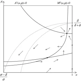
The phase plane diagram for this situation is presented in figure 4 Since in the case of all rationals playing L we are only interested in the behavior of the system within the area ML, and (a, µ) ∈ ML implies
µ < δ/(δ +σ) < 1/2 and a > (σ−δ)/σ > 0, so the only restpoints we are interested in are the crossing points (intersections) of the curves (11) and (12). The existence of those restpoints within the areasLand ML, for given payoffs and functionf, depends on the cost̺ and an aspiration level
α. We will not give precise conditions that guarantee existence of crossing points within areas L or ML here.8 Instead, the following lemma will be sufficient for our purposes (see appendix for the proof of the lemma).
Lemma 2. For any given environment with 0< ̺ < δ < α≤σ and f, the
system of equations
ψL(a, µ) = 0,
ML(a, µ) = 0 (13)
either has zero, or one or two solutions. In case where it has only one solution, this solution will be denoted byxu = (au, µu). In case where it has
two solutions, they will be denoted by xu = (au, µu)and xs= (as, µs)), with
as < au and µs< µu.
8
1 a
µ
σ δ
δ
+
σ δ σ−
[image:16.595.163.431.129.395.2]AL(a,µ)=0 ML(a,µ)=0
Figure 4: Phase plane diagram when all rationals play L.
Moreover, for any 0< δ < σ and f there is an aspiration levelα∈(δ, σ)
such that for anyα∈(δ, α)there exist̺∈(0, δ) andε∈(0, ̺) such that for any ̺ ∈ (̺−ε, ̺) the system of equations (13) has two distinct solutions, both lying within the areaL9.
From the above lemma we know that there are at most two restpoints within the areaML. It turns out that the rest pointxuisunstable, as stated
by the following proposition (see appendix for the proof of the proposition).
Proposition 1. The rest pointxu is unstable.
The other restpoint that may exist within the area ML turns out to be asymptotically stable. To show this we will use the method adopted from Palomino and Vega-Redondo [1999], which is based on the following re-sult in the theory of ordinary differential equations (see for example [Arnold, 1973, p. 198]).
Theorem 1 (Liouville’s Theorem). Let x˙(t) =H(x(t))be a dynamical sys-tem defined on a certain open subset U ⊆ Rn, where H is a differentiable
9
This of course means that these solutions lie within the areaML. One can also show that that it is possible to have a solution that lie withinML, but not withinL. It will
vector field. If S⊆U has a volume V ≡RSdx, then the volume V(t) of the setS(t) ={y=x(t) :x(0)∈S} satisfies:
˙
V(t) =
Z
S(t)
divH(x)dx,
where the divergence of the vector field H is defined as the trace of the Jacobian of H given by
divH(x)≡
n X
i=1
∂Hi(x)
∂xi
.
We now state and prove our next result.
Proposition 2. The rest pointxs is an asymptotically stable rest point.
Proof. To show that xs is an asymptotically stable rest point, we will
con-struct a set S ⊆ ML such that (i) xs ∈ S (and it is the only restpoint
inS), (ii) the vector field v points inwards on the boundary of S and (iii) div :v(x) <0 for all x ∈S. Under (i) – (iii), we know that for any t and
S(t) defined as in theorem 1 we will haveS(t)⊆S, and thus div :v(x)<0 for allx∈S(t). By theorem 1 this would imply that the volume of the set
S(t) is decreasing. Furthermore, by the Poincar-Bendixson theorem (see for example Hirsch and Smale [1974] or Hubbard and West [1991]) we know that limit sets of solutions of two dimensional differential equations either include a rest point or are closed orbits. Since the vector field v points inwards on the boundary of S, so any solution starting within S, remains there. Sup-pose its limit set is a closed orbit. Then the region enclosed by this orbit is invariant, and so is its volume. This contradicts the fact that the volume of S(t) is decreasing10. Thus limit set of any solution starting from within
our constructed S must contain xs, and so xs must be an asymptotically
stable rest point. So to prove the proposition, what remains to be shown is the existence of S. In what follows we will show how to construct a set S
satisfying the three properties (i) – (iii) postulated above.
First we present a fact and an observation characterizing the functions
ψL and ML in the neighborhood of (a
s, µs) (see appendix for the proof of
the fact).
Fact 1. In the neighbourhood of (as, µs), the partial derivatives of ψL and
ML have the following properties:
1. ψL
a(a, µ)>0 andψµL(a, µ)<0,
2. ML
a(a, µ)>0 and MµL(a, µ)<0,
10
3. −ψs
a/ψµs <−Mas/Mµs, whereψas,ψsµ,MasandMµsdenote partial
deriva-tives of ψL and ML at (a s, µs).
Observation 1. Since in the neighbourhood of(as, µs)we haveψµL(a, µ)<0
and MµL(a, µ)<0, it follows that equations ψL(a, µ) = 0 and ML(a, µ) = 0
implicitly define the functions µ =hψ(a), µ= hM(a). Moreover, as g′ψ =
−ψL
a/ψµL>0and g
′
M =−MaL/MµL>0, both those functions are increasing.
We also have g′
ψ < g
′
M, as −ψaL/ψµL < −MaL/MµL. Also, the inequalities
ψL(a, µ) < 0 and ML(a, µ) < 0 are equivalent to µ > hψ(a), µ > hM(a)
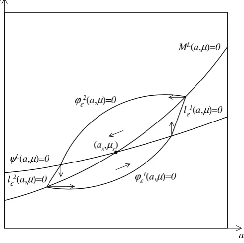
(which follows from signs of partial derivatives) (see also figure 5).
a
µ
ψL(a,µ)=0
ML(a,µ)=0
(as,µs)
ϕε2(a,µ)=0
ϕε1(a,µ)=0
lε2(a,µ)=0
[image:18.595.176.423.292.538.2]lε1(a,µ)=0
Figure 5: Construction of the setS.
The following three facts are important for further steps in the construc-tion ofS (see appendix for proofs of these facts). To state these facts, first let
K1=− M
s µ
Ms a−Mµs
, K2 = M
a µ
Ms a −Mµs
, K= 1 + max{1, K1, K2}. (14)
Notice thatK1, K2, K >0 sinceMas>0 andMµs<0. Consider the following
curves:
ϕ1ε(a, µ) = ML(a, µ)2−2κ1κ2f(α)η(ε)(a−as+µ−µs+ε) = 0,
where ε >0 and
η(ε) = max
(a,µ)∈C(Kε)g(|ψ(a, µ)|) where C(x) = [as−x, as+x]×[µs−x, µs+x]. Fact 2. If ε is close to0, then η(ε) =o(ε)>0.
Fact 3. There existsε >0such that for allε∈(0, ε)there is an intersection point (a1M(ε), µ1M(ε)) of the curves ϕ1ε(a, µ) = 0 and ML(a, µ) = 0 and an
intersection point(a2M(ε), µ2L(ε))of the curvesϕ2ε(a, µ) = 0 andML(a, µ) =
0. Moreover, these intersection points have the following properties: 1. ψL(a1
M(ε), µ1M(ε))>0 and −Kε < a1M(ε)−as <0, −Kε < µ1M(ε)−
µs<0, and
2. ψL(a2
M(ε), µ2M(ε))<0 and 0< a1M(ε)−as < Kε, 0< µ1M(ε)−µs <
Kε.
Fact 4. There exists ε >0 satisfying fact 3 and such that for all ε∈(0, ε)
1. there is an intersection point(a1ψ(ε), µψ1(ε))of the curvesϕ1ε(a, µ) = 0
and ψL(a, µ) = 0 such that M(a1
ψ(ε), µ1ψ(ε))>0, as< a1ψ(ε)< a1M(ε)
andµs< µ1ψ(ε)< µ1M(ε);
2. ifML(a, µ)>0,ψL(a, µ)>0and ϕ1ε(a, µ) = 0, thena < as+Kεand
µ > µs−Kε;
3. there is an intersection point(a2ψ(ε), µψ2(ε))of the curvesϕ2ε(a, µ) = 0
andψL(a, µ) = 0, such thatM(a2
ψ(ε), µ2ψ(ε))<0,a2M(ε)< a2ψ(ε)< as
andµ2
M(ε)< µ2ψ(ε)< µs;
4. ifML(a, µ)<0,ψL(a, µ)<0and ϕ2
ε(a, µ) = 0, thena > as−Kεand
µ < µs+Kε.
Now consider the curves
ℓ1ε(a, µ) = (µ2M(ε)−µ1ψ(ε))(a−a1ψ(ε))−(a2M(ε)−aψ1(ε))(µ−µ1ψ(ε)) = 0, ℓ2ε(a, µ) = (µ1M(ε)−µ2ψ(ε))(a−a2ψ(ε))−(a1M(ε)−aψ2(ε))(µ−µ2ψ(ε)) = 0,
which are lines going through points (a1ψ(ε), µ1ψ(ε)), (a2M(ε), µ2M(ε)) and (a2
ψ(ε), µ2ψ(ε)), (a1M(ε), µ1M(ε)) respectively. Define the sets
Sε1 = {(a, µ) :ϕ1ε(a, µ)≤0 and A(a, µ)≤0 and ML(a, µ)≤0}, Sε2 = {(a, µ) :ϕ2ε(a, µ)≤0 and A(a, µ)≥0 and ML(a, µ)≥0},
LetSε=Sε1∪Sε2∪Sε3∪Sε4. Facts 3 – 4 guarantee that there existsεsuch
that for anyε∈(0, ε) the setSε is nonempty, (as, µs)∈Sε andSε⊆C(Kε)
(refer to observation 1 and figure 5). The following lemma helps us to show that ifε < ε, then all solutions that enterSε must stay there (see appendix
for the proof of the lemma).
Lemma 3. Let ε be such that facts 3 – 4 hold. Then for any ε∈(0, ε) the vector fieldv points inwards on the boundary of the set Sε.
Notice that, sinceAa(as, µs) = 0 (as g(0) = 0) andMµ(a, µ)<0 around
(as, µs) and at (as, µs), so there is ε∗ >0 such thatAa(a, µ) +Mµ(a, µ)<0
for all (a, µ) ∈ C(ε∗). Thus the set S = Sε, where ε ∈ (0, ε∗) and is such
that facts 3 – 4 are satisfied, satisfies all the postulates at the beginning of the proof of the lemma. This completes the proof that (as, µs) is an
asymptotically stable restpoint. Now can prove Main Result 2.
Main Result 2. This is an immediate consequence of lemma 2 and proposi-tion 2. Addiproposi-tionally, by proposiproposi-tion 1 we know that there can be at most one stable restpoint in the area L. This completes the proof of Main Re-sult 2.
We end this section with the following remark.
Remark 4 (The aspiring population in an eternal flux). Consider the asymptotically stable rest point in the region ML which we have discov-ered above. Since it is a rest point,a˙ = 0. In our environment, this means that there is no player in the population who switches behavior rules at this rest point. Moreover, at this point we have that 0 < µ < 1 and therefore some aspiring players playH while others play L. Also, since this rest point is in the region ML, we know that all players using the rational rule play
3.2 Low aspiration level
Throughout this section we will assume that the aspiration level is low, that is 0< α≤δ. In this case an expression for ˙µsimplifies to the following:
˙
µ=M(a, µ) =κ2f(α)(1−a)(ξ−µ). (15)
As the following analysis will show, with low social aspirations, the relatively costly rational rule (no matter how small its associated cost may be) has no chance of survival in the long run.
3.2.1 The analysis with an initial condition in MH
Similar to the high aspiration case we will first study the behavior of the system with initial conditions in the regionMH where all rationals playH. Unlike in the case of high aspiration, there is no asymptotically stable rest point when the aspiration level is low. This is becauseM(a, µ) = 0 fora= 1, so all points lying within the set{(1, µ) :δ/(δ+σ)< µ≤1}are rest points. The following analysis and simulations show the existence of asymptotically stable sets (in forms of intervals contained in the set{(1, µ) : 0≤µ≤1}).
Main Result 3. Consider any coordination game such that0< δ < σ and an aspiration level α ∈ (0, δ]. Let X = [0,1]×[δ/(δ+σ) +ε,1]⊃ H − S,
x∈ X and let φv(t,x) be a solution of the system of differential equations
(5), (7). Thenlimt→+∞φv(t,x) = (1, µ∗), where µ∗∈[δ/(δ+σ) +ε,1].
Moreover if ̺ ∈ (0, σ2/(4(δ+σ))), then for x = (a, µ) ∈ X such that a <1 and µ > µ1 we haveµ∗
≥µ2, where
µ1 = δ δ+σ +
σ−pσ2−4̺(δ+σ)
2(δ+σ) , µ2 =
δ δ+σ +
σ+pσ2−4̺(δ+σ)
2(δ+σ) .
Proof. Obviously we have MH(a, µ) = 0 iff a = 1 or µ = 1. Moreover
MH(a, µ)≥0 andψH(a,1) =̺fora∈[0,1), soAH(a,1)>0 forµ∈[0,1).
It also holds that AH(1, µ) = 0 fora= 1 (cf. proof of lemma 1).
This shows that all points (1, µ∗
) such thatµ∗
> δ/(δ+σ) are the only rest points within the areaMH. Since there are no cycles in the areaX (as
MH(a, µ) ≥0 for all (a, µ) ∈ X and whenever MH(a, µ) = 0 it holds that
AH(a, µ) = 0) and all trajectories starting within X will remain there, so
by Poincar-Bendixson theorem we have limt→+∞φv(t,x) = (1, µ∗).
For the second part of the theorem, let us consider the crossing points of linesψH(a, µ) = 0 and MH(a, µ) = 0. To find them it is enough to solve
the quadratic equation
ψH(1, µ) =µ2(δ+σ)−µ(2δ+σ) +δ+̺= 0.
The discriminant of the equation is ∆ = σ2 −4̺(δ+σ). It is clear that
equation has two solutions
µ1 = δ δ+σ +
σ−pσ2−4̺(δ+σ)
2(δ+σ) , µ2 =
δ δ+σ +
σ+pσ2−4̺(δ+σ)
2(δ+σ) . Moreover ψH(1, µ) < 0 iff µ ∈ (µ1, µ2) so the set of points satisfying the inequalityψH(a, µ)<0 contains the set of points (1, µ), whereµ∈(µ
1, µ2).
Thus no trajectory starting from points (a0, µ0)∈ X, such thata0 <1 will
reach a rest point in this set. So any trajectory starting from any point (a0, µ0) ∈ Y = [0,1]×[µ1,1]⊂ X, such thata <1 and µ > µ1 will remain
inY (as the vector field points inwards on its boundary, everywhere apart from points where it vanishes) and will reach the rest point (1, µ∗
) such that
µ∗
> µ2.
Remark 5. Observe that µ2 → 1 and µ1 → δ/(δ+σ) as ̺ → 0. Thus the smaller ̺ we take, the bigger the area Y from where all trajectories approach restpoints of the form (1, µ∗
). In particular, if ̺ is small enough, the population starting from the state where less than a half of aspiration driven players play H will reach the state where most of them play H and there are no rationals.
3.2.2 The analysis with an initial condition in ML
In case of initial conditions within ML, the fraction of aspiration driven players playing H decreases continually over time and we are able to show that if the trajectory stays within ML, it will reach the rest point (1, µ), whereµ∈[0, δ/(δ+σ) +ε].
Main Result 4. Consider any coordination game such that0< δ < σ and an aspiration levelα∈(0, δ]. Any trajectory that starts in the are ML and remains there reaches the rest point (1, µ∗
), where µ∗
< δ/(δ+σ).
Proof. Obviously we have ML(a, µ) = 0 iff a = 1 or µ = 0. Moreover
ML(a, µ)≤0 and ψL(a,0) =̺ for a∈[0,1), so AL(a,0)>0 fora∈[0,1).
It also holds that AL(1, µ) = 0.
This shows that all points (1, µ∗
) such thatµ∗
< δ/(δ+σ) are the only rest points within the areaML. Since there are no cycles in the areaML(as
ML(a, µ)≤0 for all (a, µ)∈ ML and wheneverML(a, µ) = 0 it holds that
AL(a, µ) = 0), so for any trajectory starting withinMLthat remains there,
by the Poincar-Bendixson theorem, we have limt→+∞φv(t,x) = (1, µ∗).
converge to the rest point (1, µ∗
). Moreover, the set of trajectories that remain in the ML area is non empty, as any trajectory starting from the point (a,0) that is within ML remains there and reaches (0,0) point (as
ML(a,0) = 0).
4
Simulations
[image:23.595.156.437.283.576.2]In this section we will demonstrate how the system under consideration behaves in four different scenarios – two with high aspiration levels and two with low aspiration levels.
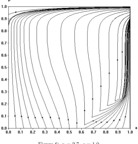
Figure 6: α= 2.7,̺= 1.0.
Our analytical results show that any qualitatively different behavior of the system depends neither on the payoffs of the game nor on the probability functions affecting willingness of individuals to change the rule or the action, but on the aspiration levelαand the cost of rationality̺. Thus in scenarios considered in this section we fix the game to the one withδ = 2 andσ = 5 and we also fix the speed adjustment parameters to κ1 = κ2 = 1. We
also consider the probability functions of the form f(x) = dx2, g(x) =
b(x2 −cx3). Parameters d, b and c are chosen to satisfy the conditions
f(σ) = 1,g(σ−̺) = 1 and g′
maximal value forα and σ−̺ is the maximal absolute difference between average payoffs of rational and aspiration driven populations).11
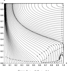
Figure 7: α= 2.15,̺= 0.1.
Since the value ofddepends only on the game, it will be fixed tod= 0.04. The value of c depends on the cost of rationality and will be calculated separately for each scenario using the same formula c = 2.0/(3.1(σ −̺)). The value of b depends on the value of c and will be calculated using the formulab= 1.0/((σ−̺)2−c(σ−̺)3).
In the first scenario we demonstrate the behavior of the system when the aspiration level and the cost of rationality are high enough to prevent the existence of rest points in the ML area. As we can see in the figure 6 the fraction of aspiration driven players playingH increases constantly until the system reaches the only rest point (1,1).
In the second scenario we demonstrate the behavior of the system when the aspiration level is above δ, but close to it and the cost of rationality is small enough to enforce the existence of rest points in the ML area. We can see in figure 7 that in this scenario most of the areaMLis the basin of
11
Figure 8: α= 1.8,̺= 0.12.
attraction of the stable rest pointxs. So most of the initial conditions lying
within the ML region remain there and lead to a stable population where rational and aspiration driven players coexist.
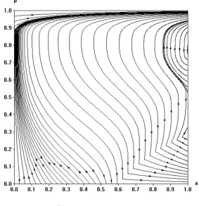
In the last two scenarios we demonstrate the behavior of the system when the aspiration level is low. In both cases we fix it to the same value and show how the behavior of the system depends on the cost of rationality. In figure 8 we can see that if̺ is small then almost all trajectories starting within MH end up in the state where rationals die out and the fraction of aspiration driven players playing H is close to 1. Moreover almost all trajectories starting withinMLend up in the state where rationals die out and the fraction of aspiration driven players playingH is close to 0.
Figure 9 shows the behavior of the system with a higher cost of rational-ity. One can observe that there are trajectories starting withinMH which end up in the state where all rationals die out and the fraction of aspiration driven players playingHis relatively small. We can also see that most of the trajectories starting within ML remain there, but reach states of various levels of fractions of players playing H. A careful look at the line a = 1 reveals the existence of stable and unstable sections. For example, for µ
Figure 9: α= 1.8,̺= 0.8.
5
Concluding Remarks
In this paper we study an evolutionary model of equilibrium and behavior-rule selection. We have kept the analysis as simple and tractable as possible by restricting attention to the simplest possible class of games where playing best response requires a rational player to gather information, the cost of which we assumed to be positive no matter how small. Players could avoid this small implementation cost of rationality by adopting an alternative and simple behavior rule, which we call the aspiring rule, which incorporates a fixed and common aspiration across all players who adopt this rule. We show that there are two stable long run outcomes where either the relatively costly rational rule becomes extinct and (if aspiration level is high enough) all players in the population achieve full efficiency, or that both the behav-ior rules co-exist and there is only a partial use of efficient strategies in the population. These findings rationalize the use of the aspiration driven be-havior in several existing studies in the literature and also helps us take a comparative evolutionary look at the two rules in retrospect.
involves dynamic systems in dimensions higher than 2. We reserve this issue for future research.
Acknowledgement We thank Sandro Brusco, Huw Dixon, Rajeeva Karandikar and Jorgen Weibull for various comments and suggestions during several stages of this research. The usual disclaimer applies.
A
Appendix
Theorem 2. Suppose that an autonomous differential equation x′
= f(x)
has a rest pointx0 = (x0, y0), its linearization has eigenvalues 0, λ, the x
-axis is the eigendirection for the eigenvalue0, they-axis is the eigendirection for the eigenvalueλand that
first nondegeneracy condition 0 is a simple eigenvalue of the lineariza-tion, the other eigenvalueλ is nonzero,
second nondegeneracy condition the coefficient p2,0 ofx2 in the Taylor
expansion ofx′
is nonzero.
Assume further thatλ <0andp2,0 >0. Then there exist unique
trajecto-ries which tend tox0 tangentially to the line of eigenvectors with eigenvalue
λfrom both sides. Moreover,
(i). these trajectories, together with x0, form a smooth curve called the
separatrix of the saddle node;
(ii). all trajectories to the left of this separatrix tend to 0 tangentially to the line of eigenvectors with eigenvalue0, forming a pony tail; and (iii). there is a unique exceptional trajectory to the right of this separatrix
which emanates from x0, also tangentially to the to the line of
eigen-vectors with eigenvalue0.
Lemma 2. It will be convenient to make the following substitutions:
d:=f(α)/(f(α−δ) +f(α)), τ :=σ/δ, υ:=̺/δ. (16) Then the system of equations (13) takes the following form:
aµ2(1 +τ)−µ+υ= 0,
Notice that the lineµ= 0 is an asymptote of both curves defined by the above equations, and so the following analysis will be conducted forµ6= 0. By solving for afrom these two equations we get
a= µ−υ
µ2(τ + 1)
a= µ−(1−d)
µ(2d−1 +µ(1−d))
(18)
Comparing the right side (forµ6= 0) we get the following quadratic equation:
µ2(d+τ) +µ(d(τ −υ−1)−τ +υ) +υ(2d−1) = 0. (19) Thus the system of equations (13) has zero, one or two solutions.
The discriminant of equation (19) is
∆=υ2(1−d)2−2υ(d2(τ+ 1) + (2d−1)(τ +d)) + (τ(1−d) +d)2. (20) Solving the inequality ∆≥0 forυ we get
υ1 = d
2(τ+ 1) + (2d−1)(τ +d)−√Γ
(1−d)2 ,
υ2 =
d2(τ+ 1) + (2d−1)(τ +d) +√Γ
(1−d)2 ,
where Γ = 4d2(d+τ)(τ + 1)(2d−1)>0 for any τ > 1 and 1/2 < d < 1. Notice also that√(Γ)< d2(τ+ 1) + (2d−1)(τ+d), as 4(1−d)2((τ(1−d) + d)2)> 0 andd2(τ + 1) + (2d−1)(τ +d)>0. Moreover d2(τ + 1) + (2d−
1)(τ+d)>(1−d)2(τ+ 1), sinced2>(1−d)2. Hence we can conclude that
∆≥0 forυ ≤υ1 and υ ≥υ2, where 0≤υ1 < υ2 and υ2 > τ + 1. Because
we restrict ourselves to 0< υ <1, the condition reduces toυ≤υ1.
To show that it is always possible to have one or two solutions within the areaLwe will first show that there is always somed∈(1/2,1) such that
υ1<1. This inequality (under our assumptions) reduces to
(d−1)2(d2(τ −2√τ + 1)(τ+ 2√τ+ 1)−2dτ(τ + 1) + (τ + 1)2)<0 and further to
(d−1)2
d− τ+ 1
τ + 2√τ + 1 d−
τ+ 1
τ −2√τ + 1
<0, ifτ 6= 2√τ+ 1
and
(d−1)2(τ+ 1) (2dτ −τ −1)>0, ifτ = 2√τ+ 1.
Let
d∗1 = τ+ 1
τ + 2√τ + 1 = 1 2+
(√τ + 1−1))2
2(τ + 2√τ+ 1) <1,
d∗2 = τ+ 1
It is easy to see that if τ −2√(τ + 1)6= 0 then either d∗
2 < 0 or d
∗
2 > 1,
depending on sign of τ −2√(τ + 1). Thus for d∈(0,1), υ1 <1 ifd > d∗
1.
So by making dbig enough one can always make sure that it is possible to choose υ =υ∗
∈ (0,1) such that system of equations (13) has exactly one solution.
After the substitution
A:=d+τ, B :=d(υ+τ), C :=υ(2d−1), (21) the equation (19) takes the form
µ2A+µ(B−A−C) +C = 0, (22) where A > 3/2, B > 1/2 and 0 < C < 1. The discriminant of the above equation is∆= (A−(B−C))2−4AC and the solutions are
µs=µ∗−
√
∆
2A, µu =µ
∗
+
√
∆
2A, (23)
where
µ∗= A−(B−C) 2A .
Since A > B (as A−B =d(1−υ) +τ(1−d)), so A−(B−C)>0. Also
B > C (as B−C =d(τ −υ) +υ). Moreover √(∆) < A−(B−C). Thus 0< µs≤µ∗ ≤µu<1−(B−C)/2A <1.
Letq :R+→Rbe a function such that q(µ) = µ−(1−d)
µ(2d−1 +µ(1−d)).
It can be easily checked that ford∈(1/2,1), q is strictly increasing, so for
as =q(µs),au=q(µu) andµs< µu we have as< au.
To see if it is possible that{xu,xs} ∈ L we will first look for conditions
onµ for which (q(µ), µ)∈ L, that is such that
q(µ)µ < q(µ)−σ/(δ+σ). (24) The inequality (24) simplifies to
µ2((2−d)τ+ 1)−µ((1−d)(3τ + 1) + 1) + (1−d)(τ + 1)<0, (25) with the discriminant
Γ =d2(5τ2+ 2τ + 1)−2dτ(3τ + 1) +τ2.
So for the inequality (24) to have two solutions it must be true thatd < dL1
ord > dL
2 where
dL1 = τ(3τ + 1−2
p
τ(τ + 1)) 5τ2+ 2τ + 1 , dL2 = τ(3τ + 1 + 2
p
τ(τ + 1)) 5τ2+ 2τ + 1 = 1−
It is easy to see thatdL
1 <1/2 anddL2 <1, so for the values ofdwe consider,
the condition forΓ >0 reduces to d∈(max(d∗
2, dL2),1).
The inequality (24) is satisfied if µ∈(µL
1, µL2), where
µL1 = (1−d)(3τ + 1) + 1−
√
Γ
2(1 +τ(2−d)) , µ
L
2 =
(1−d)(3τ+ 1) + 1 +√Γ
2(1 +τ(2−d)) Since (µL
1, µL2)→[0,1/(τ+ 1)] andµ
∗
→1/(2(τ+ 1)) whend→1, so there is d ∈ (max(d∗
2, dL2),1) and υ such that µ
∗
∈ (µL
1, µL2). Moreover there is ε > 0 such that for all υ ∈ (υ−ε, υ), µs < µu and (µs, µu) ⊆ (µL1, µL2).
Thus there is α ∈ (δ, σ) (for having d big enough one can take α close to
δ) such that for any α ∈ (δ, α) there is ̺ and ε ∈ (0, ̺) such that for any
̺∈(̺−ε, ̺) the system of equations (13) has two distinct solutionsxs,xu
such that{xs,xu} ⊆ L.
Proposition 1. The linearization of the system of differential equations (5), (7) at xu has one zero eigenvalue, so we cannot simply use it to reason
about properties of this restpoint. However we can study a linearization of the modified system of differential equations
˙
a=ψL(a, µ),
˙
µ=ML(a, µ), (26)
to reason about stability of the rest point (notice that one can view the system of linear differential equations (5), (7) as a perturbed system (26) where the perturbation preserves the signs of ˙aand ˙µ). We first prove the following fact.
Fact 5. The linearization of the system of differential equations (26) at xu
has two nonzero eigenvalues of opposite signs, that is, xu is a saddle node
of the system.
Proof. Partial derivatives of ψL andML at (au, µu) are as follows:
ψua =ψLa(a, µ)|(au,µu) = [µ
2(δ+σ)]|(
au,µu),
ψuµ=ψLµ(a, µ)|(au,µu) = [2aµ(δ+σ)−δ]|(au,µu),
Mau =MaL(a, µ)|(au,µu)= [κ2µ(f(α)−f(α−δ)(1−µ))]|(au,µu),
Mµu =MµL(a, µ)|(au,µu)
= [−κ2(f(α−δ)(a(1−µ) + 1−aµ) +f(α)(1−a))]|(au,µu).
(27)
The characteristic polynomial of the Jacobian of the vector fieldvat (au, µu)
is
with the discriminant∆= (ψu
a−Mµu)2+ 4Mauψµu. It is obvious thatψau >0,
Mau >0 and Mµu <0. We will show that ∆ >0, by showing that ψuµ ≥0.
Consider the equation
aµ2(δ+σ)−µδ+̺= 0,
satisfied by (au, µu). Solving it with respect toµ we get that
µu ≥
δ
2au(δ+σ)
(notice that by lemma 2, if there are two solutions to this equation, µu is
the bigger one). This immediately leads to conclusion thatψu µ≥0.
SinceMu
aψµu−ψuaMµu >0, so
√
(∆)>|ψu
a+Mµu|. Thus the characteristic
polynomial has two real and distinct solutions λ1 <0< λ2.
The rest of the proof of proposition 1 below is based on the proof of theorem 8.3.2 from [Hubbard and West, 1991, part II, pp 155–159], stating that if a rest point is a saddle node of a linearization then it is a saddle node.
To analyze the system we will first move the point (au, µu) to the origin
and change the basis to eigenbasis of the linearization matrix of (26). After this transformation, the system of equations (26) becomes
˙
x=λ1x+P(x, y),
˙
y=λ2y+Q(x, y),
(29)
where λ1 and λ2 are eigenvalues of the linearization of (26), P and Q are polynomials starting with at least quadratic terms from the expansion ofψL
and ML into a Taylor polynomial, and a and µ of the original system are
changed tox and y, for clarity.
Similarly, the system of differential equations (5), (7) is transformed to ˙
x=Ae(x, y),
˙
y=λ2y+Q(x, y), (30)
where
e
A(x, y) =κ1((1−c(x, y))g(λ1x+P(x, y))−c(x, y)g(λ1x+P(x, y))),
wherec(x, y) =αx+βy+au is aafter an affine transformation. Obviously
Following the proof from Hubbard and West [1991] we turn the system of differential equations (29) into first order equations, first fory as a function ofx, and then forx as a function ofy:
dy
dx = ϕ1(x, y) =
λ2y+Q(x, y)
λ1x+P(x, y), (31) dx
dy = ϕ2(x, y) =
λ1x+P(x, y) λ2y+Q(x, y)
. (32)
We do the same with the system of differential equations (30) : dy
dx = ϕe1(x, y) =
λ2y+Q(x, y)
e
A(x, y) , (33) dx
dy = ϕ2e (x, y) =
e
A(x, y)
λ2y+Q(x, y)
. (34)
The equations (31) and (33) will be considered only within areas where
λ1x+P(x, y)6= 0 (and also Ae(x, y) 6= 0). The equations (32) and (34)
will be considered only within areas whereλ2y+Q(x, y) 6= 0. Under these assumptions all those differential equations satisfy Lipschitz condition, since the right hand sides are differentiable.
From Hubbard and West [1991] we observe that trajectories of solutions to the system (29) follow the graphs of solutions to the first order differential equations (31) and (32) (with time going backwards or forward, depending on the sign ofλ1 and λ2, cf. Hubbard and West [1991]).
Similarly trajectories of solutions to the system (30) follow the graph of solutions to the first order differential equations (33) and (34) as in the neighborhood of (0,0), λ1x has the dominating effect on Ae(x, y) and g is strictly increasing.
In the analysis of the behaviour of solutions of equations (33) and (34) we will need the following notions and theorems from [Hubbard and West, 1991, part II, pp 511–515] (in what follows, I denotes an open or closed interval, possibly unbounded from either side).
Definition 1 (Lower fence). For the differential equation x′
= f(t, x), we call a continuous and continuously differentiable functionα(x) a lower fence
if α′
(t)≤f(t, α(t)) for allt∈I.
Definition 2 (Upper fence). For the differential equation x′
= f(t, x), we call a continuous and continuously differentiable functionβ(t)an upper fence if f(t, β(t))≤β′
(t) for allt∈I.
Definition 3 (Antifunnel). 12 If, for the differential equation x′
=f(t, x), over somet-intervalI,α(t) is a lower fenceand β(t) in an upper fence and
12
if α(t)> β(t), then the set of points (t, x) for t∈I with α(t)≥x ≥β(t) is called an antifunnel.
Theorem 3 (Antifunnel Theorem; Existence). 13 Let α(t) andβ(t),α(t)≤
β(t), be two fences defined for t ∈ [a, b), where b might be infinite, that bound an antifunnelfor the differential equation x′
=f(t, x). Furthermore, let f(t, x) satisfy Lipschitz condition in the antifunnel. Then there exists a solution x=u(t) that remains in the antifunnel for all t∈[a, b) where u(t)
is defined.
Suppose that λ1 > 0. We will consider the system of differential
equa-tions (33) forx < 0 and we will show that there exist at least one solution
u(x) of the system (33) that approaches point (0,0) as x increases, and moreover, that it is tangent to thex-axis.
Consider the two areas defined as follows
L1(ε, γ) = {(x, y) :−ε < x <0 and −γx2< y < γx2} L2(ε) = {(x, y) :−ε < x <0 and x < y <−x}.
We will show that there existε >0 and γ >0 such that L1(ε, γ) andL2(ε) are both backward antifunnels for the equation (33).
The equationλ1x+P(x, y) = 0 implicitly defines a curve tangent to the y-axis (which, in the neighborhood of (0,0), is exactly the same as the curve defined byAe= 0). Thus there exist ε >0 and γ >0 such thatAe(x, y)6= 0 and λ1x+P(x, y)= 0 within areas6 L1(ε, γ) and L2(ε).
First we will show that y(x) =γx2 is a lower fence. Notice that
ϕ1(x, y) =
λ2y+Q(x, y) λ1x+P(x, y)
= λ2y+Q(x, y)
λ1x
1
1− (P−(λx,y)
1)x
=
λ2y λ1x
+Q(x, y)
λ1x
1 +P(x, y) (−λ1)x
+
P(x, y) (−λ1)x
2
+ · · ·
!
.
Take y(x) =γx2. IfQ(x, y) does not have a term inx2, then for suffi-ciently smallε the first term in the first parentheses dominates the second. Otherwise both terms are linear inx. In that case, since the coefficient ofx2
inQ(x, y) is independent ofγ, we can take γ sufficiently large such that for
ε sufficiently small the first term will dominate the second. Then the sign of ϕ1(x, γx2) depends on the sign of λ1/(λ2x), so ϕ1(x, γx2) >0 and thus
e
ϕ1(x, γx2)>0. Since (γx2)′
= 2γx <0 forx <0, so for sufficiently smallε,−ε < x <0, and forγ sufficiently large, γx2 is a lower fence forϕ
1(x, y). Similarly it can
be shown that for −ε < x < 0, ε sufficiently small, and for γ sufficiently
13
largeϕe1(x,−γx2)<0, so, since (−γx2)′=−2γx >0 for x <0, −γx2 is an
upper fence forϕ1(x, y). Thus L1(ε, γ) is an antifunnel forϕ1(x, y).
The proof that there is an εsuch thatL2(ε) is an antifunnel goes along
the same lines and is easier. This is because the first term in the first parentheses is a constant and the second term is at most linear inx, and so it is dominated by the first term.
Thus, by theorem 3, for x < 0 there is a solution to the linear differ-ential equation (33) such that it remains in the antifunnels L1 and L2 and approaches (0,0). Moreover it does so tangentially to the x-axis, as it re-mains in the antifunnelL1. Sincex(t) decreases astincreases (cf. (29), (30))
so this means that there are solutions to (29) leaving (0,0) tangentially to the direction of eigenvector ofλ1.
One can show similar result forx >0 analogically, using backward anti-funnels being analogues for L1 and L2. Moreover, using (34) one can show that there are trajectories approaching (0,0) tangentially to eigenvector of eigenvalueλ2, defining antifunnels that are regions complementary to those
for equation (33) (cf. Hubbard and West [1991]).
Ifλ1<0, one can show that there are trajectories leaving (0,0)
tangen-tially to eigenvector of eigenvalueλ2 <0, and its proof is analogical to that
above, again relying on the fact that Ae(x, y) has, in the neighborhood of (0,0), exactly the same sign asλ1x+P(x, y). Thus we have shown thatxu
is an unstable rest point. This ends the proof of proposition 1.
Fact 1 of Proposition 2. To show thatψL
µ(a, µ)<0,consider the equation
aµ2(δ+σ)−µδ+̺= 0,
with (as, µs) being its solution. Solving it with respect to µwe get that
µs <
δ
2as(δ+σ)
,
(notice that here we assume that there are two solutions to this equality). Thus in the neighborhood of (as, µs) ψLµ(a, µ)<0.
The rest of the claims in parts 1 and 2 follow directly from the expressions for partial derivatives (cf. (27)).
For part 3 we first transform the inequality to the following form
ψasMµs−ψsµMas>0,
and further (forµs>0) to
−asµs(τ + 1)(2d−1)−µs(d+τ) + (2d−1)>0,
(wheredandτ are as in (16). Sinceasandµssatisfy (18), so this inequality
is equivalent to
−(µs−υµ)(2d−1)
s −