A Retrospective Comparative Study of three Data Modelling Techniques in
Anticoagulation Therapy
S. McDonald, C. Xydeas, and P. Angelov
Dept. of Communication Systems, Infolab21, Lancaster University, Lancaster, England LA14WA
[email protected], [email protected], [email protected],
Abstract
Three types of data modelling technique are applied retrospectively to individual patients’ anticoagulation therapy data to predict their future levels of anticoagulation. The results of the different models are compared and discussed relative to each other and previous similar studies. The conclusions of earlier papers, that machine learning could help anticoagulation clinicians achieve better results, are reinforced here using an extensive data set. Continuously-updating neural network models are shown to predict future INR measurements best of the three types of models presented here.
1. Introduction
Anticoagulation therapy is widely implemented by medical practitioners throughout the world in the prophylaxis of thrombosis. The British Committee for Standards in Haematology reports that only 50% of such patients in Britain actually respond to their treatment as their clinician predicts [1]. This figure indicates the inherent difficulties faced by anticoagulation clinicians. The most important clinical decisions in anticoagulation therapy are:
• Individual anticoagulant dose calculation
• Time period until next consultation
• Duration of treatment
Clinicians express the coagulability of a patient’s blood in International Normalised Ratio (INR) units. This value is based on the time taken for the blood to clot on the addition of a reagent. The aim of anticoagulation is to keep the patient’s INR readings within the appropriate therapeutic range. To make suitable therapeutic decisions the patient’s INR history is considered along with their other medication and any lifestyle changes. The role of data modelling and machine learning in anticoagulation is to support the clinician’s decision-making and to facilitate the process. In this way it is hoped that better clinical
decisions can be made with less effort. There are several existing software products that support anticoagulation clinicians and several studies into their efficacy [2, 3, 4, 5, 6]. Other studies have been undertaken to investigate the utility of particular machine learning technologies using anticoagulation data [7, 8, 9, 10, 11].
Although the models presented here are relatively simple the value of this study comes from the extensive amount of data available compared to other studies. Consequently, it is believed that these results will be more representative of the wider population of anticoagulation patients than those presented in previous studies. Three types of model are studied: polynomial, auto-regression/moving average with exogenous variable (ARMAX) [12], and neural network (NN). The INR prediction results are discussed relative to the other models in this study and relative to previous results reported in this application area.
2. Data Modelling Methods
This retrospective study uses anonymous historical anticoagulation data collected in the DAWN AC Decision Support Software as part of a benchmarking service which aims to improve anticoagulation care at participating clinics. The data is available for five clinics across five half-year periods between April 2003 and October 2005. The anticoagulation therapy histories of 19585 patients are provided, of which 2189 have less than eight clinic visits which is considered here to be too few to permit reasonable modelling of the underlying behaviour and dynamics. Typically these first eight visits occur during the first weeks of treatment (induction). Thus, data for 17396 patients is analysed in this study. This is a total of 844928 clinic visits which represents over 1.78 million patient treatment days, or 48821 patient treatment years (PTY).
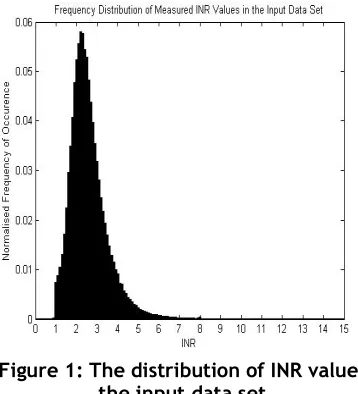
Thirty-eight attributes are available for each patient of which three are considered in this study: the current INR reading, the dose instruction in milligrams (based on the current reading and target therapeutic INR range), and the time to the next clinic visit in days (interval). The recorded INR values are restricted to the range of zero to fifteen (several higher values were truncated). This is reasonable since INR values higher than five require urgent remedial action and values over fifteen represent an almost complete inability to coagulate. The distribution of INR readings is shown in figure one below. Note that the majority of the measured INR values fall in the range 1 – 4 units.
Figure 1: The distribution of INR values in the input data set
Dose instructions lie in the range 0 to 1199mg. This should be the daily dose instruction in which case 1199mg is far too high, possibly even a lethal dose. Such errors are always present in large sets of manually-entered data. Over 99% of the dose instructions occur in the range 0 to 10mg. The clinic interval values fall between zero and 994 days. Again the upper limit here is far too high at almost three years. This is an error and perhaps represents a break in treatment followed by a later restart. More typically the clinic visit interval values are between zero and 56 days, with the majority of values falling on some multiple of seven days which suggests a weekly scheduling approach.
Such interval values mean that there is a different irregular sampling interval in each patient’s INR time series. This leads to three obvious ways of modelling: time-independent, using the test interval as an input, and interpolation to achieve regular sampling. All three are studied here. For the purposes of interpolation a daily sampling rate is selected. The INR signal is interpolated in a linear fashion, which is standard practice in anticoagulation decision support, even if it does not truly reflect the behaviour of the
INR values. Because the dose instructions are daily they are interpolated using zero-order hold, dropping to zero when ‘skip dose’ instructions have been recommended (usually when the patient is over-anticoagulated). Test intervals are meaningless as inputs in such daily models, they must be used iteratively to see the effect of a dose instruction over an extended time period. This is quite different to those models which use the test interval as an input where that input value is varied to see the predicted effect of the same dose over a different time period.
The two polynomial models are both third order, a value which is found experimentally to minimise the number of unsafe or unusable solutions. The models take the form:
p
(
x
)
=
p
1x
3+
p
2x
2+
p
3x
+
p
n+1.Pi are the parameters of the model and x is the value of the current INR reading. Training of the models is achieved by the generation of the Vandermonde matrix of the polynomial,
v
i,j=
x
in−j, and then matrix division to solve the system of equations,V
p≅
y
, forP in a least squares sense to derive the coefficients of the polynomial. One of the polynomial models is time-independent and acts directly on the irregularly-sampled data (model #1). The input to the model is the most recent INR reading and the output is the predicted next INR measurement. The second polynomial model (#2) acts on the interpolated data at a daily sampling rate. Here the current value of the INR signal is used to predict the INR reading on the next day. In this model only the final prediction before the next clinic visit is interesting since there are no actual INR measurements between visits from which a meaningful error can be calculated. Indeed, between visits the output of the previous prediction becomes the input of the next iteration, until a new measurement is made at the next visit.
An ARMAX model (#3) is used because of the presence of an exogenous (external) control variable in the system, namely the dose instruction variable. The form of the model is:
)
(
)
(
)
(
)
(
)
(
)
(
q
y
t
B
q
u
t
k
C
q
e
t
A
=
−
+
where A(q),B(q), and C(q) are polynomial coefficients respectively of the current and previous values of the output (y(t)), the dose (u(t-k)), and the independent and identically distributed random variables e(t) ~ N(0, σ2) which
selected from the most successful method of: Gauss-Newton (new direction = Hessian matrix-1 * gradient
direction), restricted Gauss-Newton (search space is bounded by a predefined tolerance value), or Levenberg-Marquardt [13, 14] (new direction = -1 * the pseudoinverse of (H + d * I) * gradient direction) where H is the Hessian, I is the identity matrix, and d is varied to find the minimum. The ARMAX model can only work on a time series that is regularly sampled.
Four standard feed-forward back-propagation neural network (NN) models are developed. Two of these model the irregularly-sampled data using INR, Dose, and Interval values as inputs to produce the predicted next INR as a single output (ie. three nodes in the input layer and one in the output layer). The other two models are used with the interpolated data and the test interval is not required as an input (two input nodes and one output). The best performing internal structure is found to be two hidden layers with three and five nodes. All the nodes have hyperbolic tangent sigmoid transfer functions. Two models are trained and then fixed before testing (one on irregularly-sampled (#4) and one (#7) on interpolated data) while the remaining two continue to have their internal connection weights and biases updated after each step (again one on each type of data: irregularly-sampled (#5) and interpolated (#6)). Backpropagation produces the Jacobean, jX, of the mean square error (MSE) performance relative to the weights and biases of each connection (X). These values are then each adjusted by the Levenberg-Marquardt [13, 14] update method:
[
]
[
jX
E
]
I
jX
x
*
2
+
+
µ
−
=
∂
where I is the identity matrixand E is a matrix of the errors. Mu is altered until the MSE performance improves and then the change in X is applied.
In each case where the model is trained and then fixed, sixty percent of the available data is used for training and the rest for testing. The data is always presented in chronological order so that testing never occurs on training data. Each of the seven models described here is applied to every patient (with at least eight clinic visits) independently, ie. these are patient-specific models. All values are normalised in the range zero to one before modelling and the predictions are unnormalised subsequently by the inverse operation.
3. Experimental Results
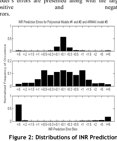
The large volume of results suggests that a frequency distribution is probably the best way to visually assess the efficacy of each model. The INR prediction errors are snapped into irregularly-sized bins
with smaller bins near zero and larger bins further away. The mean and standard deviation of each model’s errors are presented along with the largest
[image:3.612.326.527.100.343.2]positive and negative errors.
Figure 2: Distributions of INR Prediction Errors for Models #1 - #3
For model #1, subplot 1 in figure 2, around 57% of the INR prediction errors lay between -0.1 and 0.1 INR units. The errors from 92% of the total number of predictions are found in the five bins between -0.5 and 0.5 INR units. The distribution is quite symmetrical about the central bin. The mean and standard deviation of the errors produced by model #1 are very large due to the presence of relatively few extreme predictions. The second subplot in figure 2 shows just over twelve percent of predictions by model #2 produce errors in the -0.1 to 0.1 range of INR units. A similar proportion of errors fall in the -0.5 to -1 and the 0.5 to 1 bins. Only 52% of predictions produce errors between -0.5 and 0.5. Over 3% of errors are found in the two largest magnitude bins and 1.9% of the predictions give either positive or negative infinite errors. Again the distribution is almost symmetrical. Again the mean and standard deviation are rendered meaningless, this time due to infinitely large errors. It is immediately clear from the distribution in subplot 3 (figure 2) that model #3 performed extremely poorly with almost 83% of the errors falling in the extreme bins. Here 0.6% of the predictions produced infinitely large errors, positive or negative. Only 2.4% of errors lay in the range -0.5 to 0.5 INR units. The distribution is heavily biased towards large negative errors. Again, the presence of infinitely large errors renders statistical measures useless.
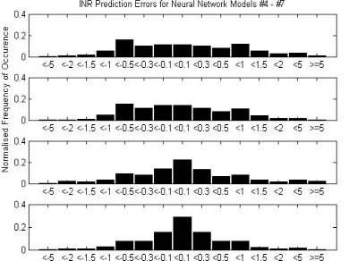
shows the results from a network which is fixed after training and operates directly on the irregularly-sampled data (model #4). 11.4% of predictions give errors of between -0.1 and 0.1 INR units. 66.7% of predictions produce errors between -0.5 and 0.5. Only 0.8% of errors have a magnitude of greater than five units. The results are quite symmetrical. The mean error for model #4 is 0.095 INR units with a standard deviation of 1.17. The largest positive error is 24.1 and the smallest negative error is -12.47. A constantly-updating network (model #5) is also used on the irregularly-sampled data. These results are shown in subplot 2 of figure 3. 14% of the INR predictions produced errors with a magnitude of less than 0.1 units, while 74.8% of errors fell in the range -0.5 to 0.5 INR units. Only 0.25% of errors had a magnitude greater than five units. Again the distribution of errors does not appear to be skewed. For model #5 the mean error is 0.0129 with a standard deviation (SD) of 0.8507. The maximum error is 13.973 and the minimum is -12.81 INR units.
Figure 3: Distributions of INR Prediction Errors for Models #4 - #7
Two neural networks are used to model the linearly-interpolated data. The first is constantly updating (model #6) and the prediction errors are shown in subplot 3 of figure 3. 22.4% of errors fall in the range -0.1 to 0.1. Errors with a magnitude of less than 0.5 account for 73.3% of all predictions, and 2.5% of errors have a magnitude greater than five INR units. The distribution is not skewed. Model #6 has a mean INR prediction error of 0.0418 with SD 0.9319. The maximum error is 38.87 and the minimum is -16.57 units. The final model (#7) is fixed after training on interpolated data. These results can be found in subplot 4 of figure 3. Here 29% of errors are very small (-0.1 < error < 0.1) and only 0.5% are very big ( |error| > 5). 82.7% of errors fall between -0.5 and 0.5 INR units. Once again, there is no disposition towards over- or under-estimation. Model #7 produces a mean
error of 0.1627 INR units (SD 1.549). The largest positive error is 28.62 and the largest negative error is -26.27 INR units.
4. Discussion
As previously stated, anticoagulation clinicians aim to keep a patient’s INR reading within an appropriate therapeutic range, which typically spans one INR unit. The most frequently-occurring range is 2 – 3 INR units and the other common ones are: 2.5 – 3.5, 3 – 4, 3.5 – 4.5, and 1.5 – 2.5. In this way errors of magnitude 0.5 INR units or less would seem to be acceptable, although smaller still is preferable.
Model #1, a third order polynomial, produces by far the greatest proportion of errors in the range -0.5 to 0.5 INR units. The distribution, plot 1 in figure 2, is closest to the ideal shape, ie. has the most prediction errors in the central bin (-0.1 to 0.1). However, the maximum and minimum errors are of the order 1052 or
1053. These values are clinically unacceptable and
render the mean and standard deviation meaningless. This is caused by an ill-conditioned [15] Vandermonde matrix where small changes in the coefficients of the system change the output drastically. Hence, small changes in the input can lead to huge changes in the output. Such sensitivity to initial conditions is one of the necessary conditions for chaotic behaviour. Not every patient’s INR signal can be modelled well by a third order polynomial, particularly when signal values are repeated in long sequences. Furthermore, this is the simplest type of model due to time- and dose-independence, and is thus the least useful to the intended application in isolation. The balance between dose instruction and interval to next test is critical to the clinician. However, if such models are used sensibly, that is rejecting predictions outside the INR input limits (zero and fifteen INR units), they could be used to reinforce the predictions produced by other models.
for the next day’s predicted INR in the absence of any real measurement. These models are dose-independent.
The third order ARMAX model, #3, works on interpolated data and uses the dose instruction as a second input. In this sense it could be very easily used in the support of anticoagulation decision making. Unfortunately, the prediction results are exceptionally poor. Almost 0.6% of the errors have infinite magnitude due to unstable (autoregressive coefficients outside the unit circle on the z-plane) or ill-conditioned models. This level of performance is unacceptable in the application. Note the strong tendency to underprediction evident in plot 3 of figure 2. Of these three models, it is clear that the time-independent polynomial model #1 performs best, with the other model #2 second, and the ARMAX model #3 a distant third.
The fixed and constantly updating neural network models that operate on irregularly-sampled data, #4 and #5 respectively, produce quite similar results. Unsurprisingly, the constantly adjusted network performs better, with reference to the error distributions, subplots 1 and 2 in figures 3 and the means and standard deviations. The current INR, dose instruction, and test interval are inputs. Both types of network always produce stable models and show a slight tendency to underestimate the following INR. 51% and 59% respectively of the errors are within acceptable limits and the maximum errors are no larger than 24.1. This compares well to the huge and/or infinite errors of the previous models but those extreme predictions are still clinically useless.
Models #6 (constantly updating) and #7 (fixed after training) operate on interpolated data. The mean and SD of model #6 lie between those of the networks of models #4 and #5 (which modelled irregularly-sampled data). Model #7, however, performs worse than all three of the other networks. Recall that this model is fixed after training and reuses predictions as inputs between clinic visits, both of which decrease the accuracy. Conversely, the best performing network models the irregularly-sampled data and is constantly adapting.
In order to meaningfully compare models #1 - #3 with the networks in models #4 - #7, the unusable means and standard deviations of #1 - #3 are recalculated only for predictions that lie in the application INR range of zero to fifteen units. The results are shown in table 1. The error statistics presented in table 1 show that, even after limiting the results set, models #2 and #3 are considerably worse than the others. Considering stability issues and mean errors the network models are preferable. The simple, time-independent polynomial model #1 could be used
alongside to further inform the decision-making process.
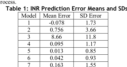
Table 1: INR Prediction Error Means and SDs Model Mean Error SD Error
[image:5.612.322.537.86.200.2]1 -0.078 1.73 2 0.756 3.66 3 8.66 11.8 4 0.095 1.17 5 0.013 0.85 6 0.042 0.93 7 0.163 1.55 Three existing studies have applied neural network models to the problem of predicting the INR response to particular dose instructions. Mayo [8] found a mean INR prediction error of 0.0927 with a standard deviation of 0.033 for a backpropagation network, representing 91.1% accuracy. For a network that was updated using a genetic algorithm the mean error was 0.0557 (sd. 0.024). These results can be compared with the neural network models #4 to #7. Mayo’s backpropagation NN produces a very similar mean error to model #4 (fixed network on irregular data), see table 1, but has a much lower standard deviation. The genetic algorithm/NN model performs better than model #4 but worse than #5 in terms of mean error. Model #6 has a mean that falls between those of Mayo’s models and model #7 performs noticeably worse. For each model, the standard deviation of the errors is much larger in this study. This is probably due to the different INR input distributions: the INR readings in [8] lay between 1.5 and 3.7 INR units compared with 0 to 15 units in this study. This should also make the modelling task easier in the earlier work. In a second study, Rennie [9] found that neural network models for individual patients predicted the next INR reading with between 48% and 82% accuracy. The mean accuracy was found to be 67.4%. Further to this a NN model was trained on the data from multiple patients and achieved between 54% and 88% (mean 70.1%) accuracy. Although the input data is not described mathematically, only patients under anticoagulation for two or more years were considered. Such patients should normally have quite a stable maintenance dose and a relatively stable INR signal. This performance seems a little worse than might be expected and certainly does not predict the INR as well as models #4 - #7 in this study, or in Mayo’s work.
Mayo’s and the network models in this study. It is possible that too many inputs can confound the modelling of a signal.
It is also interesting to compare these results with another technique. Vadher et al [11] produced a pharmacokinetic model of the dose/INR response and used Bayesian parameter estimation. Their models predicted INR values with mean errors of -0.07, 0.02, 0.03, and 0.06 INR units. These values agree very well with the results presented here and in [8]. In each of these four studies the authors concluded that it is possible to accurately predict the INR response to a given dose instruction. In two cases [7] and [9] it is concluded that the performance is better than that of the clinician. Such a comparison is not valid since the model is only concerned with accurately predicting a patient’s response over time, based on the current INR and dose and previous prediction errors. The clinician, however, must also consider varying the dose instruction to achieve the desired therapeutic INR value (or range). The INR model is ignorant of the target INR value. Thus, when the prescribed dose falls outside the desired range, one can not know whether this is due to the clinician’s inability to correctly predict the response to that dose, or that the wrong dose was selected. It is essential to remember that the model will support, and not replace, the clinician.
The instability of polynomial and ARMAX models, based on sensitivity to initial conditions, is a problem. Neural network models also have some drawbacks. The updating of the connection weights finds a solution that minimises the error given the most recent inputs and the stored history (in the weights). In this sense each new update ‘smears’ the knowledge retained from earlier updates, an effect that increases with the degree of non-stationarity of the data. Furthermore, NN models are black-box systems: deriving useful meaning from the structure or values in the model is impossible. This may affect the acceptance of any system by expert clinicians. The use of rule-based or prototype-based modelling may help to overcome both of these problems, particularly if behaviour patterns repeat over time.
Interestingly, even the best models produce relatively large errors from time to time. This is evidence of the variability of INR signals. There are many sources of noise and many unmeasured variables in the data: patient compliance with dosing instructions, interactions between the anticoagulant and other drugs (particularly Aspirin, Paracetamol, and Amiodarone), patient illnesses, measurement and data recording error, the nature of the blood flow, and the state of blood vessel walls. Most models seem capable of predicting the signal well when the signal remains in the range of INR values that dominates the
distribution. However, the extreme INR values are the most important clinically, and are thus those that need to be properly predicted. INR models must be robust in the face of noise. Finally, the utility and performance improvement shown by multi-patient models is highlighted in [9]. This must be considered in future developments because it is the only way to have a useful model at the start of treatment, ie. for patients with no INR history.
5. Conclusions
The use of polynomial and ARMAX-type models in predicting INR values is dangerous because such systems can be unstable or can become unstable for certain inputs. Used carefully they could further inform the predictions of other models. Neural networks perform well in comparison and are always stable. Of the all the networks the continuously-updating model of irregularly-sampled data performed best. Indeed, models fixed after training always performed worse. As concluded in previous similar studies, it seems reasonable from the results presented in this paper to suggest that machine learning could be used to assist anticoagulation clinicians. These models must, however, be constantly adapting and robust to the noise in the INR signal. They should also perform equally well for the infrequent extreme INR readings and the more frequent stable readings. Furthermore, a useful multi-patient model must be found for the induction of new patients to anticoagulation therapy.
Future work could investigate estimation and removal of noise, the use of rule-based modelling, and perhaps the use of fuzzy methods. A multi-patient model should be developed.
6. Acknowledgements
The authors would like to thank all the participating patients and clinics for their support in allowing the use of their data during this study. Furthermore, cordial thanks are extended to the helpful and friendly staff at the sponsoring company, 4S Dawn Clinical Software.
7. References
[2] L. Poller, D. Wright, and M. Rowlands, “Prospective Comparative Study of Computer Programs used for Management of Warfarin” J Clin Path 1993, 46, pp. 299-303 [3] P.H. Abbrecht, T.J. O’Leary, and D.M. Behrendt, “Evaluation of a computer-assisted method for individualized anticoagulation: retrospective and prospective studies with a pharmacodynamic model” Clin Phar Ther 1982, 32, pp. 129-136
[4] A. Kubie, A.H. James, J. Timms, and R.P. Britt, “Experience with a computer-assisted anticoagulation clinic”
Clin Lab Haem 1989, 11(4), pp.385-391
[5] B. Vadher, D.L. Patterson, and M. Leaning, “Evaluation of a Decision Support System for Initiation and Control of Oral Anticoagulation in a Randomised Trial” BMJ April 26 1997, 314(7089), pp. 1252-1256
[6] T.P. Oppenowski, E.T. Murray, H. Sandhar, and D.A. Fitzmaurice, “External quality assessment for Warfarin dosing using Computerised Decision Support Software” J Clin Path 2003, 56, pp. 605-607
[7] S. Byrne et al, “Using Neural Nets for Decision Support in Prescription and Outcome Prediction in Anticoagulation Drug Therapy” Unpublished, submitted to the European Conference on Artificial Intelligence, 2000
[8] M. Mayo, “An Adaptive Computer-Based System for the prescription of Warfarin” Undergraduate dissertation 2002, Dept. of Computer Science, University of Canterbury, Christchurch, New Zealand
[9] L. Rennie, “Using Machine Learning to Predict the Effects of Warfarin on Heart Patients” Undergraduate dissertation 2004, Dept. of Computer Science, University of Canterbury, Christchurch, New Zealand
[10] M. Carney et al, “The Benefits of Using a Complete Probability Distribution when Decision Making: An Example in Anticoagulant Drug Therapy” Technical Report 2005, Computer Science Department, Trinity College, Dublin
[11] B. Vadher et al, “Prediction of the INR and maintenance dose during the initiation of Warfarin therapy” Br J Haem
1999, 48, pp. 63-70
[12] E.J. Hannan, “The Identification and Parameterization of ARMAX and State Space Forms” Econometrica 1976, 44, pp. 713-723
[13] K. Levenberg, "A Method for the Solution of Certain Non-Linear Problems in Least Squares." Quart Appl Math
1944, 2, pp. 164-168
[14] D. Marquardt, “An Algorithm for Least-Squares Estimation of Non-Linear Parameters” SIAM J Appl Math
1963, 11, pp. 431-441
[15] G. Peters and J.H. Wilkinson, “Inverse Iteration, Ill-Conditioned Equations and Newton’s Method” SIAM Review