On the Probability Distribution of Economic Growth

On the Probability Distribution

of Economic Growth

Pär Stockhammar and Lars-Erik Öller

Department of Statistics, Stockholm University S-106 91 Stockholm, Sweden

E-mail: par.stockhammar@stat.su.se

Abstract

Normality is often mechanically and without su¢ cient reason assumed in econometric models. In this paper three important and signi…cantly heteroscedastic GDP series are studied. Heteroscedasticity is removed and the distributions of the …ltered series are then compared to a Normal, a Normal-Mixture and Normal-Asymmetric Laplace (NAL) distributions. NAL represents a reduced and empirical form of the Aghion and Howitt (1992) model for economic growth, based on Schumpeter’s idea of creative de-struction. Statistical properties of the NAL distributions are provided and it is shown that NAL competes well with the alternatives.

Keywords: The Aghion-Howitt model, asymmetric innovations, mixed normal- asym-metric Laplace distribution, Kernel density estimation, Method of Moments estima-tion.

1. Introduction

In the Schumpeterian world growth is driven endogenously by investments into R&D, leading to better products, which initially capture monopoly pro…ts. The quality improvements occur randomly over time. The main contributions to endogenous growth are Romer (1986) and Lucas (1988). They both argued that the underlying growth is determined by the accumulation of knowledge, with occasional setbacks. Other important papers on endogenous growth are: Segerstrom, Anant and Dinopoulos (1990), Grossman and Helpman (1991) and Aghion and Howitt (1992, henceforth AH).

"When the amountnis used in research, innovations arrive randomly with a Poisson arrival rate n, where >0is a parameter indicating the productivity of the research technology."

This was later also assumed in e.g. Helpman and Trajtenberg (1994) and Maliar and Maliar (2004). The latter study recognizes short waves, but unlike the present study neither accepts negative shocks. There are many real life exam-ples that justify negative shocks, e.g. unsuccessful investments in physical or human capital, bad loans, losses when old investments become worthless and political con‡icts. By negative (destructive) random shocks we try to mimic the setbacks in our reduced univariate approach. Moreover, all the models in the quoted works are speci…ed in the time domain, while density distributions are the object of this study.

It is found that some important growth series exhibit heteroscedasticity, which is removed using a …lter described in Öller and Stockhammar (2007). The …ltered series are shown to be homoscedastic but leptokurticity and positive skewness prevail, rendering a hypothesis of normality dubious.

In the Poisson process the time between each shock is exponentially distrib-uted with intensity ; see Appendix A. In this study however, we have used the exponential distribution to describe the amplitude of the shocks. When is small we expect infrequent but large shocks and vice versa. This intuitive way to describe the shocks accords well with modern economic theory. Specif-ically, to allow for negative or below average shocks, we have used the double exponential (Laplace) distribution obtained as the di¤erence between two ex-ponentially distributed variables with the same value on the parameter :The Laplace distribution is symmetric around its mean where the left tail describes below average shocks and vice versa. Due to the asymmetries in these series we have allowed the exponential distribution to take di¤erent s in the two tails, giving rise to the asymmetric Laplace (AL) distribution. This is our main model candidate. The asymmetric properties of the AL distribution have proved ap-pealing for modelling currency exchange rates, stock prices, interest returns etc. see for instance Kozubowski and Podgorski (1999, 2000) and Linden (2001).

Another plausible explanation is that the long growth series have passed through alternating regimes over the years. Every such regime has its own normal distri-bution giving rise to a Normal Mixture (NM) distridistri-bution, which is our alterna-tive hypothetical distribution, because it is hard to see how this could support the AH hypothesis.1 _{The NM distribution, where skewness and leptokurtocity} are introduced by varying the parameters, was used as early as the late nine-teenth century by e.g. Pearson (1895).

It was found that the excess kurtosis in AL models is too large for the …ltered (and un…ltered) growth series. The AL (and hence AH) could therefore not be the only source of shocks, so Gaussian noise is introduced. AL distributed inno-vations are combined with normally distributed shocks leading to the weighted

mixed normal-AL (NAL) distribution. The NAL distribution is capable of gen-erating a wide range of skewness and kurtosis, making the model very ‡exible. We also consider a convolution of the N and AL distributions. The parameters are estimated using the method of moments (MM).

This paper is organized as follows. The data and the …lter are presented in Section 2, and a model discussion together with the proposed model in Sec-tion 3. SecSec-tion 4 contains the estimaSec-tion set-up and a distribuSec-tional accuracy comparison. Section 5 concludes.

2. The data

In this paper the important US GDPq(quarterly) 1947-2007, UK GDPq 1955-2007 and the compound GDP 1960-1955-2007 series of the G7 countries2 _{are studied} as appearing on the websites of Bureau of Economic Analysis (www.bea.gov), National Statistics (www.statistics.gov.uk) and of OECD (www.oecd.org), re-spectively. All series are quarterly and seasonally adjusted, …nal …gures, from which we form logarithmic di¤erences, henceforth "growth" for short. In order for the N, NM and NAL distributions to properly describe the rather complex properties, long series are required. The above series are the longest quarterly GDP series available, and the G7 series is based on a large number of observa-tions, albeit not as long as the US and UK ones. The latter series were found signi…cantly heteroscedastic in Öller and Stockhammar (2007). The ARCH-LM test rejected the null hypotheses of homoscedasticity also in the compound G7 GDP series with a p-value of 0:0004. Heteroscedasticity implies an unequal weighting of the observations leading to ine¢ cient parameter estimates. Het-eroscedasticity is removed using the …lter in ibid.:

y_t =sy

2 6 6 6 4

yt Pt+=t y /k

HP( ) _{(2 )} 1Pt+ =t yt

Pt+

'=t y'/k 2 1=2

3 7 7 7

5+y; (2.1)

where yt =Di¤ ln GDPi (i =U S; U K; G7), t =k ; :::; n , k is the

win-dow length, = (k 1)=2, y_t is the …ltered series and sy and y are the

es-timated standard deviation and arithmetic mean ofyt; respectively. HP( ) is

the Hodrick-Prescott (1997) …lter designed to decompose a macroeconomic time series into a nonstationary trend component and a stationary cyclical residual.

Given a seasonally adjusted time series zt, the decomposition into unobserved components is

zt=gt+ct;

wheregt denotes the unobserved trend component at timet, andct the

unob-served cyclical residual at timet. Estimates of the trend and cyclical components are obtained as the solution to the following minimization problem

min

[gt]Nt=1

(_N X

t=1 c2_t+

N

X

t=3

(₄2gt)2

)

; (2.2)

where₄gt=gt gt 1andgminis the HP-…lter. The …rst sum of (2.2) accounts

for the accuracy of the estimation, while the second sum represents the smooth-ness of the trend. The positive smoothing parameter controls the weight between the two components. As increases, the HP trend become smoother and vice versa. Note that the second sum, (₄2_{gt), is an approximation to the}

second derivative ofgat timet. For quarterly data (the frequency used in most business-cycle studies) there seems to be a consensus in employing the value

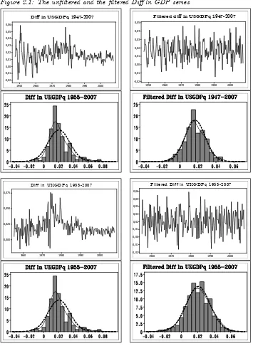
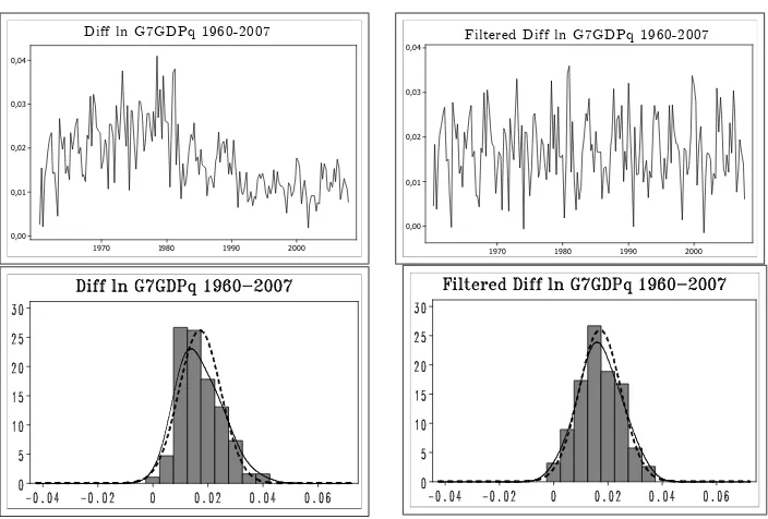
= 1600. Figure 2.1 shows the Di¤ ln US, UK and G7 GDP series before and after the …ltering3.

3_{The …ltering was done usingk= 15and the standard value for quarterly data, = 1600.} The bottom panels in Figure 2.1 show the frequency distributions of the un…ltered and …ltered data, respectively. The dashed line is the N distribution with the same mean and variance as those of the series. The solid line is the Kernel density estimate

c

fh(x) =

1

nh

n

X

i=1

K xi x

h

wherehis the bandwidth andK( )is the Kernel function. In this study we have used the Gaussian Kernel,K(u) = 1

2 e

u2

2 ;and the Silverman (1983) "Rule of Thumb" bandwidth

b

h= 4b

5

3n

!1=5

1:06_bn 1=5

Figure 2.1: The un…ltered and the …ltered Di¤ ln GDP series

2000 1990 1980 1970 1960 1950 0,06

0,05

0,04

0,03

0,02

0,01

0,00

-0,01

-0,02

Diff ln USGDPq 1947-2007

2000 1990 1980 1970 1960 1950 0,05

0,04

0,03

0,02

0,01

0,00

-0,01

-0,02

Filtered diff ln USGDPq 1947-2007

2000 1990 1980 1970 1960 0,075

0,050

0,025

0,000

Diff ln UKGDPq 1955-2007

2000 1990 1980 1970 1960 0,06

0,05

0,04

0,03

0,02

0,01

0,00

-0,01

-0,02

2000 1990 1980 1970 0,04

0,03

0,02

0,01

0,00

Diff ln G7GDPq 1960-2007

2000 1990 1980 1970 0,04

0,03

0,02

0,01

0,00

Filtered Diff ln G7GDPq 1960-2007

The …lter e¤ects on the four moments of US, UK and G7 GDP growth series can be seen in Table 2.1. Period 1 represents the quarters 1947q1-1977q2 (US), 1955q1-1980q2 (UK) and 1960q1-1983q4 (G7). Period 2 contains 1977q3-2007q4 (US), 1980q3-2007q4 (UK) and 1984q1-2007q4 (G7).

Table 2.1: Filter e¤ ects on the moments of the Di¤ ln US, UK and G7 GDP series

b b b b b b b b

Period 1 2 1 2 1 2 1 2

yt;U S 0:018 0:016 0:013 0:008 0:27 1:63 1:00 5:51 y_{t;U S} 0:017 0:017 0:011 0:011 0:05 0:22 0:30 0:42 yt;U K 0:024 0:016 0:018 0:007 0:45 0:53 0:40 0:49 y_{t;U K} 0:020 0:020 0:014 0:014 0:11 0:16 0:71 0:35 yt;G7 0:022 0:013 0:008 0:004 0:06 0:51 0:16 0:40 y_t;G7 0:017 0:017 0:008 0:008 0:01 0:16 0:31 0:24

3. Model discussion

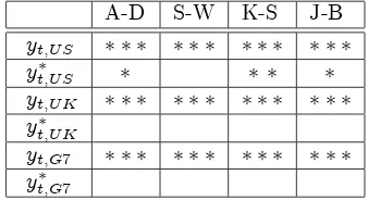
The un…ltered series in Figure 2.1 do not appear to be normal. Table 3.1 shows that the …lter brings them closer to normality

Table 3.1: Filter e¤ ects on the normality of the Di¤ ln US, UK and G7 GDP series

A-D S-W K-S J-B

yt;U S y_{t;U S} yt;U K y_{t;U K} yt;G7 y_t;G7

In Table 3.1 , and represent signi…cance at the 10% , 5% and 1% levels, resp ectively, for the null hyp othesis of norm ality. Four com m only used norm ality tests are rep orted, w here A -D , S-W , K -S and J-B are the A nderson-D arling, Shaphiro-W ilk, K olm ogorov-Sm irnov and Jarque-Bera test, resp ectively. T hese tests are based on very di¤erent m easures and can therefore lead to di¤erent conclusions.

The failure to reject normality in every entry is surprising if we again take the Figures 2.1 into consideration, where …ltered data have fatter tails than the normal distribution. According to e.g. Dyer (1974) the power of these tests is generally low, especially for small samples. Note that the K-S and A-D, J-B statistics for the US reject the null hypotheses of normality. At least for the US series it seems worthwile to see if there are other distributions that better …t the data. Considering the low power of the tests we will try the same for the UK and the G7 series. The normal distribution remains an alternative hypothesis.

With long time series there is a nonnegligible risk of distributional changes over time. One can argue that data have passed through a number of di¤erent regimes, not completely eliminated by the …lter (2.1). Every such regime could be N distributed but with di¤erent means and variances. The …ltered US GDP in Figure 2.1 still shows a small hump in the right tail, which may indicate that the data are characterized by at least two regimes, each one N distributed. Given the relatively few observations, the number of regimes is here restricted to two. Moreover, the homoscedasticity test did not detect non-constancy of variances, so even two regimes with di¤erent variances could be hard to detect. The introduction of di¤erent means and variances for the regimes render it possible to introduce skewness and excess kurtosis in the NM distribution. The probability distribution function (pdf) of the NM distribution is:

fN M(y_t; ) = w

1p2

exp

(

(y_{t 1})2 2 2

1

)

+1 w

2p2

exp

(

(y_{t 2})2 2 2

2

)

where consists of the parameters(w; 1; 2; 1; 2)and where0 w 1is the

weight parameter. If this hypothesis provides the best …t, then the AH model gets no support from the data.

Our main hypothesis for growth is a reduced form of the AH model. In this model endogenous growth is driven by creative destruction in which the under-lying source is innovations, assumed to be the result of the stochastic arrival of new technologies modelled as a Poisson process. The arrival rate itself is a¤ected by the share of the labour force engaged in research as well as by the Poisson probability of an innovation (research productivity). Each owner of a patent is assumed to have a temporary monopoly of the product lasting until it is replaced and destroyed by a better product.

AH speci…es an entire simultaneous model. This paper looks at a reduced, univariate model, where both positive andnegative shocks hit production ex-ogenously. The drawback with this approach is that the origin of the innovations cannot be identi…ed. The AH model tested in this paper simply assumes that growth is driven by a process, which is the sum of two (one positive, one nega-tive) exponentially distributed random shocks. The distribution of the di¤erence of two exponential random variables is Laplace (L) with pdf:

fL(yt; ) = 1 2 exp

jy_{t j}

; (3.2)

where = ( ; ); ₂Ris the location parameter and >0is the scale parame-ter. The L distribution (which is sometimes also called the double exponential distribution) has been used in many …elds: engineering, …nance, electronics etc, see Kotz et al. (2001), and the references therein. The L distribution is sym-metric around its mean ( ) with V ar(y) = 2 2 and excess kurtosis = 3. It thus has fatter tails than the N distribution, but it lacks an explicit shape para-meter, making it rather in‡exible. Also, the excess kurtosis is restricted to the constant value (3), no matter what the kurtosis in the data. Table 2.1 shows the kurtosis in Laplace variables is way too large for the …ltered growth series in this study (_b= 0:07for the US,_b= 0:19for the UK and_b= 0:29for the G7). Clearly, the AL as representing the AH model cannot alone explain the data.

The AH model can be modi…ed by allowing it to have a second stochastic com-ponent in the sense that its empirical counterpart is buried in Gaussian noise. We thus combine (3.2) with a N distribution via a weight parameter w. The mixture was introduced by Kanji (1985) to …t wind shear data using the Laplace Normal (LN) mixture distribution speci…ed by:

fLN(yt; ) = w

p

2 exp

(

(y_t )2 2 2

)

+(1 w)

2 exp

jy_{t j}

for ₁ < yt < 1 and for the parameters: 1 < < 1; 0 w 1 and >0: In (3.3) the L and N distributions have the same mean and variance. This case can be generalized. Jones and McLachlan (1990) assumed di¤erent variances and showed that this leads to an even better …t than Kanji’s. The characteristics of this density are shown in Figure 3.1.

Figure 3.1: LN densities

0.05 0.025

0 -0.025

100

80

60

40

20

0

w=1 w=0.9 w=0.5 w=0 The Weighting

0.05 0.025

0 -0.025

70

60

50

40

30

20

10

0

fi=0.05 N(0.017,0.011) fi=0.005

Normal-Laplace mixtures (w=0.5)

T he upp er panel in Figure 3.1. show s di¤erent weightings of the two com p onents in the N orm al-Laplace m ixture distribution (w ith =0:017; =0:011; =0:005). T he lower panel show s the pure

N(0:017;0:011)distribution together w ith two m ixture distributions w ith w=0:5; =0:05and = 0:005resp ectively.

McGill (1962) who proposes an Asymmetric Laplace (AL) distribution of the form

fAL(yt; ) =

8 > < > : 1 2 exp n_y

t o _ify

t

1 2 exp

n _y

to _ify

t >

; (3.4)

where again is the location parameter, for which the median is the Maxi-mum Likelihood (ML) estimate, and = ( ; ; ): This distribution is nega-tively skewed if > ;and vice versa for < . If = the AL collapses to the L distribution. In AL, is the parameter of shocks weaker than the trend and that of stronger shocks than the trend. If ₆= then Schumpterian shocks that lead to weaker than trend growth behave di¤erently from stronger growth shocks. During the last couple of decades, various forms and applica-tions of AL distribuapplica-tions have appeared in the literature, see Kotz et al. (2001) for an exposé. Linden (2001) used an AL distribution to model the returns of 20 stocks, where and were shown to be highly signi…cant. Another recent paper is Yu and Zhang (2005) who used a three-parameter AL distribution to …t ‡ood data.

The AL arises as the limiting distribution of the random sum (or di¤erence) of independent and identically, exponentially distributed random variables with …nite variances. An advantage of the AL distribution is that, unlike the L distri-bution, the kurtosis is not …xed. The AL distribution is even more leptokurtic than the L distribution with an excess kurtosis that varies between three and six (the smallest value for the L distribution, and the largest value for the ex-ponential distribution). Another advantage of the AL distribution is that it is skewed (for ₆= ), conforming with the empirical evidence in Figure 2.1. To this distribution we are adding Gaussian noise. To the authors´ best knowledge this distribution has not been used before for macroeconomic time series data. We assume that each shock is an independent drawing from either a N or an AL distrubution. The probability density distribution of the …ltered growth series (yt) can then be described by a weighted sum of N and AL random shocks, i.e:

fN AL(y_t; ) = _pw 2 exp

(

(y_t )2 2 2

)

+(1 w)

8 > < > : 1 2 exp n_y

t o _ify

t 1 2 exp n yt o

ify_t >

; (3.5)

for three di¤erent values of the weight parameterw.

Figure 3.2: NAL densities

0.05 0.025

0 -0.025

50

40

30

20

10

0

w=1 w=0 w=0.5

The Weighting

Figure 3.2 show s a pureN(0:017;0:011), an AL(0:01;0:02;0:017)distribution (w=1 and w=0 re-sp ectively) and a com p ound of these two com p onents w ithw=0:5:N ote the discontinuity at . The AH hypothesis also accords with the assumption that each shock is a ran-dom mixture of a N and an AL distributed component. We then arrive at the convoluted version suggested by Reed and Jorgensen (2004). Instead of using the AL parameterization in (3.4) they used:

fAL (yt; ) =

8 < :

+ expf ytg ifyt 0

+ expf ytg ifyt >0

(3.6)

which was convoluted with a N distribution giving the following pdf:

fc N AL(yt; ) = ₊ y_t

R yt +R +yt (3.7)

Figure 3.3: c-NAL densities

3 2 1 0 -1 -2 -3 1

0

alfa=10, beta=1 alfa=1, beta=10 alfa=beta=2

Figure 3.3 show s c-N A L densites using =0:017; =0:011, ( ; )=(10;1);(1;10):and ( ; )=(2;2),

resp ectively.

The c-NAL distribution has the advantage of being more parsimonous than NAL. Whether it is more suitable to describe economic growth is the issue of the next Section.

4. Estimation and distributional accuracy

In this section we will …t all four distributions (N, NM, NAL and c-NAL) in order to …nd out which one best describes the data. The …ve parameters in the NM distribution (3.1) will be estimated using the method of moments (MM) for the …rst four moments of the same. A close distributional …t is important in density forecasting. As noted by e.g. Fryer and Robertson (1972), the method of maximum likelihood breaks down for this model. Unfortunately the choice of MM excludes model selection criteria such as the AIC and BIC. This is compensated by elaborating distributional comparisons using several statistical techniques. The noncentral moments of (3.1) are given in Appendix B. Equating the theoretical and the observed …rst four moments using the …ve parameters yields in…nitely many solutions4. A way around this dilemma is to …x 1 to

be equal to the observed mode, which is here approximated by the maximum value of the Kernel function of the empirical distribution(maxfK(yi)). In the

presence of large positive skewness we can expect ₁ to be smaller than , and vice versa. Here _{b1;U S}; _{b1;U K} and _b1;G7 are substituted for maxfK(yU S) = 0:0142, maxfK(yU K) = 0:0196 and maxfK(yG7) = 0:0159. The observed

moments and the corresponding MM parameter estimates for the …ltered series (using the above values for _{1;U S}, _{1;U K} and _1;G7) are given in Table 4.1.

Table 4.1: Sample moments and estimated parameters of the NM assumption5 Sample noncentral moments Estimated NM parameters

E(y_t) E(y_t2) E(y_t3) E(y_t4) w_{b b2 b}1 b2

US 0:0168 0:0004 1:1 10 5 _{3:4 10} 7 _{0:833 0:030 0:010 0:005}

UK 0:0205 0:0006 2:1 10 5 _{8:1 10} 7 _{0:919 0:030 0:015 0:011}

G7 0:0171 0:0003 8:0 10 6 _{2:0 10} 7 _{0:866 0:024 0:008 0:006}

The log likelihood function of the NAL distribution is:

lnL( ) = w

"

n 2ln 2

2

Pn

t=1(yt ) 2

2 2

#

+ (1 w)

2

4 nln (2 ) +

1 2

Pn

t=1(yt ) I(yt E(yt)) nln (2 ) +₂1 Pn_t=1( y_t) I(y_t > E(y_t))

3 5

However, ML is in this case cumbersome, if at all possible, so again the pa-rameters are estimated by the method of moments. This also enables a fair comparison with the NM and the c-NAL distributions. The formulae of the noncentral and central moments of (3.5) are given in Appendix B. There are …ve parameters and only four moment conditions, so equating the theoretical and the observed …rst four moments will not give a unique solution. We now …x to be equal to the ML estimate with respect to in the AL distribution, that is the observed median,mdc. Here _{bU S}; _{bU K} and _bG7 are substituted for

c

mdU S = 0:0156, mdcU K = 0:0203 and mdcG7 = 0:0167. The parameter values

that satisfy the moment conditions are:

Table 4.2: Estimated NAL parameters Estimated parameters

b

w _b b b

US 0:711 0:012 0:006 0:014

UK 0:828 0:015 0:018 0:017

G7 0:939 0:008 0:008 0:020

Table 4.2 shows that the Gaussian noise component dominates. In the US and G7 series b is much smaller than b; which indicates that growth shocks that are weaker than trend have a smaller spread than above trend shocks. Together with a mean growth larger than zero this ensures long-term economic growth.

Reed and Jorgensen (2004) provided some guidelines on how to estimate the c-NAL parameters in (3.7) using ML techniques. To be consistent and to make fair comparisons, the parameters are here again estimated using MM. Ibid. also supplied the …rst four cumulants, and in order to …nd the MM parameter

estimates we provide the …rst four noncentral moments in Appendix B. Note that the c-NAL distibution has four parameters so there is no need to …x one of the parameters to …nd an unique MM solution. The MM estimates are given in Table 4.3, which shows that c-NAL does not capture the asymmetry (_bis very close tob), cf. Table 4.2.

Table 4.3: Estimated c-NAL parameters Estimated parameters

b b b b

US 0:017 0:009 197:0 198:0

UK 0:021 0:010 140:1 136:0

G7 0:017 0:007 498:2 498:8

Figure 4.1 shows the estimated NAL and c-NAL distributions together with the benchmark N distributions and the smoothed empirical GDP series. The graphs, especially of the US distributions, reveal the discontinuity at_b, result-ing in a poignant peak, as discussed in connection with Figure 3.2.

Figure 4.1: Distributional comparison

0.04 0.02

0 -0.02

50

40

30

20

10

0

Kernel US N(0.0168, 0.011) NAL US

0.06 0.04 0.02 0 -0.02 30

25

20

15

10

5

0

Kernel UK N(0.0205, 0.014) NAL UK

The UK

0,05 0,04 0,03 0,02 0,01 0,00 -0,01 -0,02 50

40

30

20

10

0

Kernel G7 N(0.0171, 0.008) NAL G7

The G7

We have chosen to compare the ordinates of the empirical distributions and the hypothetical N, NM, NAL and c-NAL distribution for 1000 points, however dropping points outside the interval(_b 4_b;_b+ 4_b). Table 4.4 shows the dis-tributional …t for the three hypothesis. Four accuracy measures are used. The Root Mean Square Error, RMSE, is here de…ned as:

RM SE=

v u u u u t

1000_X

i=1

h

fK(y_i) fb(y_i)i

2

1000 ;

for the US.

Percentage error measures are widely used but they also have their disadvan-tages. They are unde…ned atfK(yi) = 0, and they have a very skewed

distrib-ution for fK(yi) close to zero.The median absolute percentage error measure,

MdAPE, de…ned as:

M dAP E=median

0

@100 fK(yi) fb(yi)

fK(y_i)

1 A;

is here, because of the asymmetry, a better measure than its close relative, the MAPE (de…ned as 100_n Pn_i=1 fK(y_i) fb(y_i) /fK(y_i) ):Yet another disad-vantage is that positive errors are counted heavier than negative ones. This is the reason why so-called "symmetric" measures have been suggested (Makridakis, 1993). One is the Symmetric Median Absolute Percentage Error, sMdAPE

sM dAP E=median

0

@200 fK(yi) fb(yi)

fK(y_i) +fb(y_i)

1 A:

Hyndman and Koehler (2006) suggested the Mean Absolute Scaled Error, MASE, de…ned as:

M ASE = 1

1000

fK(yi) fb(yi)

1 999

1000_X

i=2

fK(y_i) fK y_{i 1} :

Ibid. showed that this measure is widely applicable and less sensitive to ouliers and small samples than the other measures.

Table 4.4: Distributional accuracy comparison

RMSE MdAPE sMdAPE MASE

US N(0:0168;0:0111) 1:76 16:65 16:73 15:38

US NM 1:41 13:98 13:19 15:59

US NAL 1:73 9:07 9:12 12:68

US c-NAL 1:59 14:25 14:43 14:11

UK N(0:0205;0:0145) 0:65 13:00 13:63 9:46

UK NM 0:59 15:46 14:99 8:66

UK NAL 0:45 9:47 9:50 6:77

UK c-NAL 0:58 15:02 14:80 7:99

G7 N(0:0171;0:0077) 2:21 18:69 20:13 14:60

G7 NM 1:64 11:07 10:55 11:78

G7 NAL 1:20 8:65 8:99 9:00

G7 c-NAL 1:70 12:27 11:61 12:55

The NAL distribution using the parameter values in Table 4.2 is superior to the N, NM and the c-NAL distribution according to every measure, except RMSE for the US where, as expected, the discontinuity peak has a large impact on the measure. NAL shows on average 27.6%, 29.2% and 48.3% better …t for the US, UK and G7, respectively (comparing with the benchmark N distribution). Comparing to the NM distribution, NAL is an improvement with on average 15.5% , 30.2% and 21.7% for the US, UK and G7. Finally, the NAL is on av-erage a 18.8%, 27.6% and a 27.4% improvement over the c-NAL distribution. According to this numerical comparison, the US, UK and G7 GDP series could be looked upon as samples from a NAL distribution with the parameter esti-mates in Table 4.2. In other words, the AH hypothesis of economic growth could be correct, if we accept that shocks are either Poisson (AL) or N distributed, with N dominating.

Kernel estimation is based on subjective choices both of function and of band-width. But so are goodness of …t tests and it is well known that tests based on both approaches have low power. To be on safer ground we have chosen also to test the histograms using three di¤erent numbers of bins. We then get unique critical values for these tests which enable calculation of p-values. Table 4.5 re-ports the p-values of the 2_{tests using 10, 15 and 20 bins when testing the null}

hypotheses H0;1 : y N, H0;2 : y NM,H0;3 :y NAL and H0;4 : y

c-NAL.

Table 4.5: The 2 goodness of …t test

H0;1:y N H0;2:y NM H0;3:y NAL H0;4:y c-NAL

Bins 10 15 20 10 15 20 10 15 20 10 15 20

US 0:03 0:01 0:04 0:13 0:05 0:15 0:20 0:22 0:27 0:06 0:04 0:07

UK 0:91 0:70 0:83 0:84 0:34 0:57 0:71 0:64 0:32 0:90 0:72 0:88

While the power of these tests is low, they still indicate that the NAL distribu-tion …ts growth best.

5. Conclusions

The hypothesis that economic growth could be described by a reduced Poisson model is not strongly contradicted by data. The Laplace distribution is unable to describe the asymmetric and just slightly leptokurtic shape. A mixed Normal-Asymmetric Laplace (NAL) distribution is introduced and is shown to better describe the density distribution of growth than the Normal, Normal Mixture, convoluted NAL and Laplace distributions. This paper thus, from a new angle, supports the hypothesis that innovations arriving according to a Poisson process play an important role in economic growth, as suggested by e.g. Helpman and Trajtenberg (1994) and Maliar and Maliar (2004). But one has to accept that most shocks are Gaussian. Since according to the AH hypothesis, measures the productivity of only positive shocks (research productivity), the parameter could be given the same interpretation. On the other hand, would measure the strength of regimes of low productivity or downright destructive shocks. Thus, our technique provides a way to estimate these qualities, and perhaps to compare di¤erent economies.

NAL implies a decomposition of the shocks into an AL and an N part. The mean, variance, skewness and the fatness of the tails stand in relation to the …ve parameters in the NAL distribution, and are estimated using MM on the …rst four moments. The moment generating function and the …rst four central and noncentral moments of the NAL distribution are provided. Because of the close distributional …t, the NAL distribution is a good choice for density forecasting of GDP growth series, or for that matter of any series with these features. The NAL distribution could also be used for conditional density forecasts applying priors on the parameters and , but that merits another study.

Acknowledgments

Appendix A, The Poisson process

LetN(t)be the process counting the number of innovations in a period of time [0; t]. Let

T0; T1; :::be given by

T0= 0; Tn= infft:N(t) =ng:

ThenTnis the time point of then:th arrival. Now, de…neXnas the length of the inter-arrival timeTn Tn 1;whereX1 is exponentially distributed parameter :

P(X1> t) =P(N(t) = 0) =e t:

The distribution of the inter-arrival timeX2;conditioned onX1:

P(X2> tjX1=t1) =P(no arrival in (t1; t1+t]jX1=t1):

Because of independence of the two events ’arrivals in[0; t1]’ and ’arrivals in(t1; t1+t]:

P(X2> tjX1=t1) =P(no arrival in (t1; t1+t]) =e t:

Thus,X2 too is exponentially distributed. In fact, it follows by induction thatXn is expo-nentially distributed forn 1 :

P(Xn+1 > tjX1=t1; :::; Xn=tn)

= P(no arrival in (t1+:::+tn; t1+:::+tn+t]) =e t:

Now, suppose thatfUj; j= 1;2; :::gare i.i.d. exponential random variables with rate , that is .

P(Uj> t) =e t:

LetT0 = 0andTn=Tn 1+Un forn 1. Think ofUn as the time between innovations.

The counting processN(t) is de…ned as follows: Forn = 1;2; :::, N(t)< n i¤t < Tn: In other words,N(t)< nif the time of then th innovation occurs aftert. This is su¢ cient information to …nd the distribution function ofN(t)for any value oft 0. In fact,Tn has a gamma distribution forn 1. Clearly this claim is true for n= 1, since ( ;1) is the exponential distribution. Suppose the claim is also true forn kwherek 1, and consider the casen=k+ 1. Now writingfnfor the density function ofTn, convolution (withTn y) yields:

fk+1(Tn) =

Z 1 1

fk(y)f1(Tn y)dy=

Z 1 1

k

(k)y

k 1_e y _e (Tn y)_dy

=

k+1_e Tn

(k)

Z ₁

1

yk 1dy;

which is the ( ; k+ 1)density function, and

P(Tn t) =

Z ₁

t

( u)n 1

(n 1)! e

u_du:

Repeatedly integrating by parts forn= 0;1;2; :::we get

P(N(t) n) =P(N(t)< n+ 1) =

n

X

k=0

( t)k

k! e

so thatN(t)has a Poisson distribution with mean t. Since theXn’s are i.i.d., for anyn,Tn is independent ofXnfor anyk > n. In other words, the counting afterTnis independent of what has occurred beforeTn:Therefore the Poisson process restarts itself at each arrival time

Tn, hence the process is regenerative. All in all this means that the Poisson process can be simulated as the sum of exponentially distributed random numbers.

Appendix B, Theoretical moments

The noncentral moments of the Normal mixture distribution (3.1) are given by

E(Yn) = w

1 p 2 n X k=0 n k n

1 + ( 1)ko n₁ k2(k 1)=2 k₁+1 k+ 1

2 +

1 w

2p2

n X k=0 n k n

1 + ( 1)ko n2 k2(k 1)=2

k+1 2

k+ 1

2

and speci…cally the …rst four moments are

E(Y) = w 1+ (1 w) 2

E(Y2) = w 21+ 21 + (1 w) 22+ 22

E(Y3) = w 31+ 3 1 21 + (1 w) 32+ 3 2 22

E(Y4) = w 41+ 6 21 21+ 3 41 + (1 w) 42+ 6 22 22+ 3 42 :

The cdf of the NAL distribution (3.5) is given by:

F(yt; ) =

8 < :

w yt ₊1 w

2 exp

n_y

t o _ify

t

w yt _{+ (1 w) 1} 1

2exp

n_y

t o _ify

t > ,

where ( )denotes the cdf of the standard normal distribution.

The noncentral moments of (3.5) are given by

E(Yn) = pw

2 n X k=0 n k n

1 + ( 1)ko n k2(k 1)=2 k+1 k+ 1

2 +

(1 w)

" 1 2 n X k=0 n

k ( 1)

k n k k+1_{k! +} 1

2 n X k=0 n k

n k k+1_k!

#

:

E(Y) = w + (1 w) + 2

E(Y2) = w 2+ 2 + (1 w) 2+ ( ) + ( + )

E(Y3) = w 3+ 3 2 + (1 w) 3+3

2 2 2

2 2 ₊

3 2

2_{+ 2 + 2} 2

E(Y4_{) = w} 4_{+ 6} 2 2_{+ 3} 4 _{+ (1 w)} 4_{+ 2 3} 2 ₆ 2_{+ 6} 3 3 ₊

2 3+ 3 2 + 6 2+ 6 3 :

Note that the mean of the NAL distribution can be written as

E(Y) = + (1 w)

2 ;

which clearly shows the obvious fact that positively skewed distributions ( > ) will have a mean larger than and vice versa. The central moments are

E(Y) = 0

V ar(Y) = w 2+ (1 w)

"

(1 w)

2 +

2₊ 2 _{(3 +w)}

4

#

(Y) = 1 4 7

3_{+ 3} 2 ₃ 2 ₇ 3 3w( )

4

h

( + )2+ 2 2i

w2_{( )}

4

h

( + )2 2 2i w

3_{( )}3

4

(Y) = 3 16 39

4_{+ 20} 3 _{+ 10} 2 2_{+ 20} 3_{+ 39} 4

3w

4 5

4_{+ 8} 3 _{+ 5} 4 ₂ 2 2 ₄ 4₊ 2 ₆ 2 ₂ 2

+4 2 2+ 2 3w

2_{( )}2

8 7

2_{+ 10 + 7} 2_{+ 8} 2

3w3_{( )}2

4

h

( + )2 2 2i 3w

4_{( )}4

16 :

The …rst four noncentral moments of the c-NAL (3.7) are:

E(Y) = +1 1

E(Y2_{) =} 2₊ 2 2 ₊2 ( 1)₊ 2

2 +

2

2

E(Y3) = 1

3 3 6

3_{+ 6} 2_{( 1) + 3} 2 _{2 2 +} 2 2₊ 2

+ 3 _{6 6 3} 2 2₊ 2 ₊ 3 3_{+ 3} 2

E(Y4) = 1

4 4 24

4_{+ 24} 3_{( 1) + 12} 2 2 _{2 2 +} 2 2₊ 2

+4 3 6 6 3 2 2+ 2 + 3 3+ 3 2 + 4 24 24 + 12 2 2+ 2 4 3 3+ 3 2

References

Aghion, P. and Howitt, P. (1992) A model of growth through creative destruc-tion. Econometrica,60, 323-351.

Aghion, P. and Howitt, P. (1998) Endogenous growth theory. The MIT press, Cambridge.

Dyer, A. R. (1974). Comparisons of tests for normality with a cautionary note. Biometrika, 61, 185-189.

Fryer, J. G. and Robertson, C. A. (1972) A comparison of some methods for estimating mixed normal distributions,Biometrika, 59, 639-648.

Grossman, G. and Helpman, E. (1991) Quality ladders in the theory of growth. Review of Economic Studies, 63, 43-61.

Helpman, E. and Trajtenberg, M. (1994) A Time to Sow and a Time to Reap: Growth Based on the General Purpose Technologies. Centre for Economic Re-search Policy, working paper no. 1080.

Hodrick, R. J. and Prescott, E. C. (1997) Postwar U.S. business cycles: An empirical investigation. Journal of Money, Credit and Banking, 29, 1-16.

Hyndman, R. J. and Koehler, A. B. (2006) Another look at measures of forecast accuracy. International Journal of Forecasting, 22, 679-688.

Jones, P. N. and McLachlan, G. J. (1990) Laplace-normal mixtures …tted to wind shear data. Journal of Applied Statistics, 17, 271-276.

Kanji, G. K. (1985) A mixture model for wind shear data. Journal of Applied Statistics, 12, 49-58.

Kotz, S. Kozubowski, T. J. and Podgorski, K. (2001)The Laplace distribution and generalizations: a revisit with applications to communications, economics, engineering, and …nance. Birkhäuser, Boston.

Kozubowski, T. J. and Podgorski, K. (1999) A class of asymmetric distributions. Actuarial Research Cleraring House,1, 113-134.

Kozubowski, T. J. and Podgorski, K. (2000) Asymmetric Laplace distributions. The Mathematical Scientist, 25, 37-46.

Linden, M. (2001) A model for stock return distribution. International Journal of Finance and Economics, 6, 159-169.

Lucas, R. E. (1988) On the Mechanics of Economic Development. Journal of Monetary Economy, 22, 3-42.

Makridakis, S. (1993) Accuracy measures: theoretical and practical concerns. International Journal of Forecasting, 9, 527-529.

McGill, W. J. (1962) Random ‡uctuations of response rate. Psychometrika, 27, 3-17.

Öller, L-E. and Stockhammar, P. (2007) A heteroscedasticity removing …lter. Research Report 2007:1, Department of Statistics, Stockholm university.

Pearson, K. (1895) Contributions to the mathematical theory of evolution, 2: skew variation. Philosophical Transactions of the Royal Society of London (A), 186, 343-414.

Reed, W. J. and Jorgensen, M. A. (2004) The double Pareto-lognormal distri-bution - A new parametric model for size distridistri-butions. Communications in Statistics: Theory and Methods,33(8), 1733-1753.

Romer, P. M. (1986) Increasing Returns and Long-Run Growth.Journal of Po-litical Economy, 94, 1002-1037.

Schumpeter, J. A. (1942)Capitalism, Socialism and Democracy. Harper, New York.

Segerstrom, P. Anant, T. Dinopoulos, E. (1990) A Shumpeterian model of the product life cycle. American Economic Review, 80, 1077-1091.

Silverman, B. W. (1986) Density estimation for statistics and data analysis. Chapman and Hall, London.