Munich Personal RePEc Archive
On the measurement of market power in
the banking industry
Delis, Manthos D and Staikouras, Christos and Varlagas,
Panagiotis
12 June 2008
Online at
https://mpra.ub.uni-muenchen.de/14038/
On the measurement of market power in the banking industry
Matthaios D. Delis, Christos K. Staikouras
*,
Panagiotis T. Varlagas
Athens University of Economics and Business, 76 Patision Street, 104 34, Athens, Greece
Abstract
This paper compares the estimates of the two most widely used non-structural models for market power measurement in banking, namely the conduct parameter method and the revenue test, as applied to a panel of Greek banks over the period 1993-2004. We also propose a dynamic reformulation of these models within a panel data context, in order to address possible statistical problems associated with the dynamic nature of bank-level data. The results suggest that both static methods provide lower estimates of market power relative to their dynamic counterparts. Therefore, the inclusion of some dynamics in the models, even though it increased estimation complexity, helped to reveal some collusive behavior of banks.
JEL Classification: G21; L10; P20
Keywords: Market power estimation; Conduct parameter method; Revenue test; Greek banking sector
*Corresponding author. Tel.: (+30) 210 82 03 459; fax: (+30) 210 82 28 816.
1. Introduction
In the banking sector, prudential regulation and competition policy are in many
respects intertwined, while the soundness and stability of the system may in various ways
be influenced by the degree of competition and concentration. Enhanced competition may
have a deleterious impact on stability if it causes banks’ charter value to drop, thus
reducing the incentives for prudent risk-taking behavior. A more concentrated system,
inasmuch as it implies the presence of a few relatively large banks, is more likely to display
a “too big to fail” problem, by which large banks increase their risk exposure anticipating
the unwillingness of the regulator to let the bank default in the event of insolvency
problems (Hughes and Mester, 1998). Any market failure, inefficiency, or anticompetitive
conduct among banks is likely to impose more severe costs throughout the economy than
would similar defects in many other industries; thus it becomes particularly important to
understand the causes and consequences of competition in the banking industry. In this
respect, the first and most important step is the robust estimation of the degree of
imperfectly competitive conduct.
Recent trends in empirical industrial organization have popularized the use of
non-structural approaches to measure market power. These approaches, that came to be known
as the new empirical industrial organization (NEIO) models, provide empirically
implementable techniques for the analysis of non-competitive behavior in production and
cost structure. The way to these approaches has been paved by a number of forerunners,
with the two most popular models being those of Bresnahan (1982) and Lau (1982), and
Panzar and Rosse (1987). Bresnahan and Lau (BL), in a line of research termed conduct
distinction between marginal revenue and price. On the other hand, in the Panzar and Rosse
(PR) model, market power is measured by the extent to which changes in factor prices are
reflected in revenue. In other words, this revenue test (RT) involves estimating a
reduced-form equation relating gross revenue to a vector of input prices and other control variables.
While each of the two approaches nurtures its own theoretical discourse, they should not be
viewed as mutually exclusive but, more eclectically, as complementary tests.
Whereas there is fairly extensive application of these models to banking, there is a
limited body of work that compares their results. The purpose of this study is to fill this
gap, using a panel dataset of Greek banks during the period 1993-2004. Furthermore, we
propose a dynamic reformulation of the static versions of the CPM and the RT within a
dynamic panel data context. The most common motivation for also using a dynamic
approach is the statistical importance of accounting for short-run dynamics in the data.
Further, the formulation solves the inference problem when using non-stationary data
(Steen and Salvanes, 1999). Finally, the dynamic nature of the Greek banking industry and
certain changes in the regulatory environment may bias the resulting implications if only
static models are considered.
We present and describe some important dynamic factors of the Greek banking
sector, such as the patterns of consolidation and concentration, the changes in the
regulatory framework, and the liberalization process that occurred during the sample
period. The presence of these factors may lead to different adjustment costs, which in turn
make static models inadequate. Indeed, the results suggest that both static methods (CPM
and RT) tend to provide lower estimates of market power compared to their dynamic
anticompetitive conduct (e.g. Corts, 1999), this has important implications for public and
private policy-makers alike.
The rest of the paper is structured as follows. Section 2 presents the two theoretical
non-structural models applied in the current study, and Section 3 is then devoted to the
analysis of the empirical static and dynamic versions of these models. Section 4 outlines
the institutional structure of the Greek banking system and offers a discussion on the
dataset. Section 5 presents and discusses the empirical evidence of applying the models to
the Greek banking sector, while some conclusions are offered in the final section.
2. Theoretical framework
The literature on the measurement of competition can be divided into two major
streams: structural and non-structural. The structural approach embraces the
structure-conduct-performance and the efficiency hypotheses. These two models investigate,
respectively, whether a highly concentrated market causes collusive behavior among the
larger banks, resulting in superior market performance, or whether it is the efficiency of
larger banks that enhances their performance. Although these hypotheses lack formal
theoretical support by traditional microeconomic theory, they have frequently been
employed empirically in the banking industry (e.g. Evanoff and Fortier, 1988; Bourke,
1989).
However, owing to several deficiencies arising from the application of the structural
approach,1 developments in industrial organization, as well as the recognition of the need
to endogenize the market structure, many empirical studies followed a new course. The
1
novelty to competition evaluation has emerged under the impulse of the NEIO approach
(Carlton and Perloff, 2005). This approach, pioneered by Iwata (1974) and strongly
enhanced by the papers of Bresnahan (1982, 1989), Lau (1982), and Panzar and Rosse
(1987), tests competition and the use of market power, and stresses the analysis of banks’
competitive conduct in the absence of structural measures. Specifically, each of these
techniques attempts to measure the competitive conduct of banks without explicitly using
information on the structure of the market.
The first model, the Iwata model, allows the estimation of conjectural variation
values for individual banks supplying a homogeneous product in an oligopolistic market
(Iwata, 1974). This measure, to the best of our knowledge, has been applied to the banking
industry only once, by Shaffer and DiSalvo (1994), for a duopolistic banking market (in
South Central Pennsylvania).2 They find that banks’ conduct is imperfectly competitive,
but closer to perfect competition than one would expect, given the very high degree of
concentration in the market.
2.1. The conduct parameter method (CPM)
The second model, which has been applied to the banking sector in a number of
studies, is based on the procedure first suggested by Bresnahan (1982) and Lau (1982) and
further elucidated in Bresnahan’s (1989) survey of the NEIO.3 It requires the estimation of
a simultaneous-equation model, where a parameter representing the degree of market
power of firms is included. The basis of the test is the established principle that, in
equilibrium, profit-maximizing firms will choose prices or quantities such that marginal
2
cost equals their perceived marginal revenue, which coincides with the demand price under
perfect competition and with the industry’s marginal revenue under perfect collusion. As
such, the key parameter in this test is interpreted as the extent to which the average firm’s
perceived marginal revenue schedule deviates from the demand schedule, thus representing
the degree of market power actually exercised by the firms in the sample.
In this respect, consider a non-competitive industry in which N banks produce a
homogeneous output Q, facing a market demand function of the following stylized form:
Q = D (P, Z, α) + ε (1)
where D is the demand function, P is the market price of industry output Q, Zis a vector of
exogenous variables affecting demand (often including some variable measuring the
general economic activity), α is the demand parameter vector, and ε is a stochastic
disturbance.
On the supply side, the representative bank i, (i {1, 2,…, N}) is assumed to
maximize profits by solving the following one-shot game in output level:
∈
max pi qi – C (qi,ωi) (2)
where (for the ith bank), qi is the output level, pi is the respective price imposed, C is the
cost function (which for now is homogeneous across all banks in the industry), and wi is the
price vector of inputs. The optimality condition corresponding to this problem is given by
the following inverse supply relation:
( , ) i
i i
i
q
Q P
P MC q w Q
q Q Q
⎛∂ ⎞⎛∂ ⎞
= − ⎜ ⎟⎜
∂ ⎝∂ ⎟⎠
⎝ ⎠ (3)
where MC is the marginal cost function.
3
As is evident from the last equation, an integral part of the solution is the elasticity
concept /
/
i
i i
dQ Q dq q
λ ≡ , that is the conjectural variation coefficient of the NEIO literature. As
λi moves farther from zero, the conduct of bank i moves farther from that of a perfect
competitor. Thus, the (average) conjectural variation coefficient will reveal what kind of
imperfectly competitive behavior characterizes the market, and there is no need to impose
any a priori restriction on it. In other words, it is not necessary to assume a certain conduct
beforehand and test for its propriety.
Moreover, in Eq. (3), represents the semi-elasticity of market demand,
that is
( / )
Q P∂ ∂Q
( ) /
Q h
Q P
≡ ∂ ∂
, which is a function of aggregate output and other exogenous
variables (Bresnahan, 1982). Shaffer (1993) describes the banking industry’s marginal
revenue function as industry price P plus h( ) . Yet, a bank’s perceived marginal revenue is
generally not equal to the industry’s marginal revenue. In fact, the perceived marginal
revenue for bank i equals P+λih( ). The range of possible values of the conjectural variation elasticity λi is given by (0,1). In the special case of the Cournot behavior,
, and λ / i
Q q
∂ ∂ =1 i is simply the output share of the ith bank. In the case of perfect
competition, λi = 0; under pure monopoly, λi =1; and, finally, λi < 0 would imply pricing
below marginal cost and could result, for example, from a non-optimizing behavior of
banks. Clearly, aggregation implies that the average value of λi across all banks equals the
industry’s conjectural elasticity, defined as L, the latter having the same properties as λi.
Thus, this framework provides a benchmark, which can be used to identify the actual
2.2. The revenue test (RT)
The PR (1987) approach (initially developed by Rosse and Panzar, 1977) for
measuring market power relies on the premise that each bank will employ a different
pricing strategy in response to a change in input costs, depending on the market structure in
which this bank operates. In other words, market power is measured by the extent to which
changes in factor prices (unit price of funds, capital, and labor) are reflected in revenue.
The authors define a measure of competition, the H-statistic, as the sum of the elasticities of
the reduced-form revenue function with respect to factor prices. Thus, the H-statistic
represents the percentage variation of the equilibrium revenue derived from an infinitesimal
percent increase in the price of all factors used by the firm.
Panzar and Rosse (1987) show that this statistic can reflect the structure and
conduct of the market to which the firm belongs. They assert that the H-statistic is negative
when the competitive structure is a monopoly, a perfectly colluding oligopoly, or a
conjectural variations short-run oligopoly; an increase in input prices will increase marginal
costs, reduce equilibrium output, and subsequently reduce revenue.4 Under perfect
competition, where banks’ products are regarded as perfect substitutes of one another, the
Chamberlinian model, based on free entry of banks and determining not only the output
level but also the equilibrium number of banks, produces the perfectly competitive solution,
as demand elasticity approaches infinity. Thus, in this case, the H-statistic is equal to unity.
Shaffer (1982) shows that the H-statistic is also unity for a natural monopoly operating in a
perfectly contestable market and also for a sales-maximizing firm that is subject to
4
In the case where the monopolist faces a demand curve of constant price elasticity (i.e. e > 1) and where a constant returns to scale Cobb–Douglas technology is employed, Panzar and Rosse proved that H is equal to
breakeven constraints. Consequently, an increase ininput prices raises both marginal and
average costs without altering the optimal output of a bank. Exit from the market will
evenly increase the demand faced by each of the remaining banks, thereby leading to an
increase in prices and total revenue by the same amount as the rise incosts (i.e. demand is
perfectly elastic). Finally, if the H-statistic is between zero (inclusive) and unity
(exclusive), the market structure is characterized by monopolistic competition. Under
monopolistic competition, potential entry leads to contestable market equilibrium, and
income increases less than proportionally to the input prices, as the demand for banking
products facing individual banks is inelastic.
When applying the RT to assess banks’ market conduct, various assumptions about
banks’ production activity have to be made. First, the methodology requires assuming that
banks are treated as single-product firms, producing intermediation services by using labor,
physical capital, and financial capital as inputs. Second, one needs to assume that higher
input prices are not associated with higher quality services that may generate higher
revenue, since such a correlation may bias the computed H-statistic. Yet, if one rejects the
hypothesis of a contestable competitive market, this bias cannot be too large (Molyneux et
al., 1996). Among other underlying assumptions inherent in the PR model, we can mention
that: (a) banks are profit-maximizing firms; (b) the performance of these banks needs to be
influenced by the actions of other market participants; (c) the cost structure is
homogeneous; and (d) the price elasticity of demand is greater than unity (see also De
Bandt and Davis, 2000). Finally, a limitation of the RT is that any monopsony power or
upward-sloping aggregate supply curve of any essential input (such as deposits) would
prices (and hence equilibrium revenues) as a function of scale, would tend to yield higher
values of H and thereby mask any market power present on the output side, in contrast to
the CPM (Shaffer, 2004).
Despite these assumptions, the RT is a valuable tool in assessing market conditions,
mainly owing to its simplicity and transparency, without lacking efficiency. Moreover, data
availability becomes much less of a constraint, since revenue is more likely to be
observable compared to output prices. Also, by utilizing bank-level data, this approach
allows for bank-specific differences in the production function. In addition, the
non-necessity to define the location of the market a priori implies that the potential bias caused
by the misspecification of market boundaries is avoided; hence for a bank that operates in
more than one market, the H-statistic will reflect the average of the bank’s conduct in each
market.5
3. Empirical specification
This section aims to identify robust econometric procedures for applying both
non-structural models of market power described above. As Bresnahan (1989) states, only
econometric problems, not fundamental theoretical problems, could cloud inference on the
empirical results of these models. To this end, the econometric methodology to be followed
is afforded particular consideration.
3.1. CPM
5
The general empirical problem in studies relying on a CPM is the identification of
the elasticity concept L. Using the results of Bresnahan (1982) and Lau (1982), Shaffer
(1999) suggests a structural econometric model that combines separate demand and supply
functions including cross-equation restrictions. A necessary and sufficient condition for the
identification of L is that the demand function must not be separable in at least one
exogenous variable that is excluded from the marginal cost function. Following this view,
we specify the following linear demand function:
0 1 2 3 4 5 6
Q=a +a P+a Y+a Z+a PY+a PZ+a YZ (4)
where Y is an exogenous variable that affects demand. Such a demand function, which
includes three cross-product terms to improve flexibility,6 can be interpreted as a first order
local approximation of the true aggregate demand function. The exogenous variable Z is
critical for the solution of the identification problem and is generally chosen as the price of
a substitute. Notice that the demand function is specified at the aggregate level. Since we
are considering the single product case, i is well defined. i
Q=
∑
q 7Turning to the supply side of the model, we follow Shaffer (1999) who specifies a
marginal cost function out of a generalization of the minflex Laurent functional form
(which in turn is a generalization of a standard translog cost function) as follows:
[
]
2 51 4 5 0 1 2
3
/( ) i[ ln (ln ) ln ]
i i
j i
C
P L Q Y a Z b b q b q b
q
α α − ω
=
= − + + + + + i +
∑
j ij
(5)
6
Applications of the Bresnahan-Lau method in the banking industry have favored linear demand functions with one or two cross-product terms (Shaffer, 1999; Toolsema, 2002; etc.). Sjoberg (2004) uses a log-linear demand function, with one cross-product term (namely price of output times the exogenous variable), while Uchida and Tsutsui (2005) use a log-linear demand function with a number of explanatory variables, mainly corresponding to the quality of loans. We too have undertaken a log-linear demand function; however the changes in the coefficients on L are negligible.
7
Regarding the functional form imposed on the supply relation, the differentiation in
the literature is broader than in the respective one imposed on the demand relation.
According to the purpose of each study, the cost function has been given a linear, minflex
Laurent, translog, generalized Leontief, or Fourier functional form. The appropriate choice
rests on the assumptions of each study, the number of outputs specified, and the level of
flexibility required. We have relied on the generalization of the minflex Laurent since, as
Barnett and Lee (1985) suggest, even though models produced from second order Taylor
series expansions (such as the translog and the generalized Leontief) can be rendered both
flexible and regular at the median data point, that regularity usually quickly disappears as
the recent-periods boundary of time series datasets is approached. The minflex Laurent
model also can be rendered both flexible and regular at the median data point. However,
doing so with this function assures simultaneously that the model’s region of regular
behavior actually expands as the recent period boundary is approached. As a result, with
time series (and hence with panel) data, the minflex Laurent possesses substantial
advantages over the Taylor series specifications for conventional modeling purposes.8
Most of the usual properties of a cost function pose no specific requirements for the
parameters of the above supply equation. Symmetry and concavity do not involve any of
the coefficients,9 while monotonicity involves but does not constrain the coefficients on the
input prices. The property of linear homogeneity in factor prices implies . We
tested for linear homogeneity after performing the regressions; however, in all models the
3
1
0 j j
b
=
=
∑
8
For the transformation of the minflex Laurent model to our partially restricted Laurent specification and its advantages, see Shaffer (1999).
9
above hypotheses are not rejected at the 5 per cent level. Therefore, we do not impose any
initial restrictions. Finally, note that the measurement of the term , as well as the
dependent variable at the bank level, while not consistent with the profit-maximizing
solution (since a quantity game was considered), allows for heterogeneity in marginal costs
and in the price setting policy, respectively (on this issue see Tsutsui and Uchida, 2002 and
Sjoberg, 2004).
/ i
C qi
For L to be correctly specified in Eq. (5) it is necessary to treat the input prices as
exogenously given. This assumption seems reasonable, at least as far as the markets for
labor and physical capital are concerned, because banks face intense competition for these
inputs from other banks as well as non-bank firms. The market for funds will also be
treated as competitive based on the argument that depositors today have many other
tempting saving options (such as government and corporate bonds and the stock markets),
which exert a competitive pressure upon banks’ deposit rate policy. To the extent that this
is not true, i.e. that bank have some degree of market power in the deposit market, it has
been shown (Shaffer, 1999) that this will not escape identification and that it will simply be
misattributed to the asset side (consequently L will be strengthened).
For empirical implementation purposes, the CPM has to be embedded within a
stochastic framework. Thus, we assume that Eqs. (4) and (5) are stochastic owing to errors
in optimization. Introducing the additive disturbance terms in System {(4), (5)}, the latter is
specified as:
[
]
0 1 2 3 4 5 6
5 2
1 4 5 0 1 2
3
/( ) [ ln (ln ) ln ]
t t t t t t t t t t t
it
it t t t it it j jit it
j it
Q a a P a Y a Z a PY a PZ a Y Z
C
P L Q Y a Z b b q b q b u
q
ε
α α − ω
=
= + + + + + + +
= − + + + + + +
∑
+The disturbance vectors ε and u are assumed to be iid as multivariate N ~ (0, Σ), where Σ is
a positive definite matrix.
As discussed previously, equations in the latter system are interrelated, because of
the underlying CPM, through the endogeneity of the semi-elasticity of market demand,
which appears in the supply equation. Thus, we should employ a system estimator such as
nonlinear three-stage least squares (3SLS), generalized method of moments (GMM)10 or
full information maximum likelihood (FIML). We have applied all three methodologies,
with the results being similar, yet we have resorted to the 3SLS method (as most of the
relevant literature) for two main reasons. First, the FIML estimator is the asymptotically
efficient estimator only under the assumption of normally distributed residuals (see
Amemiya, 1977). We tested for normality using the Jarque-Bera statistic, which is
significant at the 1 per cent level, thus ruling against normality. Second, use of different
instruments does not significantly alter the results in the 3SLS case, while in the GMM case
the variability is larger. Therefore, we proceed with the estimation of System (6) using a
3SLS procedure.
A crucial feature of the CPM is that the variables involved are usually characterized
by short-run dynamics, which are not accounted for in the static equations. Further, a
reformulation of the static model to a dynamic one may help with the inference problem
when using non-stationary data or when severe autocorrelation in the demand equation is
present (Toolsema, 2002). Steen and Salvanes (1999) developed a dynamic version of the
Bresnahan and Lau model, based on an error-correction (ECM) framework. They applied it
to the French market for fresh salmon, using time series data. Toolsema (2002) opted for
demand equation and difficulty in identifying a purely exogenous Z variable (so as the
demand function will not be separable in Z) are problems that she could not overcome, thus
failing to estimate the model. We have closely followed her approach and indeed
multicollinearity seems to be a major problem when using time series data.
Given the above, we opt for the following dynamic representation of the demand
equation (autoregressive-distributed lag model):
0 1 1 1 1 2 2 1 3 3 1
4( ) 4 ( ) 1 5( ) 5 ( ) 1 6( ) 6 ( ) 1
t l t t l t t l t t l t
t l t t l t t l t t
Q a a Q a P a P a Y a Y a Z a Z
a PY a PY a PZ a PZ a YZ a YZ ε
− − − − − − = + + + + + + + + + + + + + − + (7)
which is derived as a static conditional demand equation, assuming the same technology as
in the static case and with dynamics resulting from an AR(1) disturbance.11 As we do not
impose the implied common factor restrictions, the dynamics may be thought of as an
empirical approximation to some more general adjustment process (Blundell and Bond,
1998). This is equivalent to identifying the short-run relationships, which are of main
interest in this study.12
Similarly, we specify the dynamic supply equation of the CPM as:
5
* * 2
, 1 0 , 1 0 1 2
3 5
2
, 1 0 1 , 1 2 , 1 , 1
3
[ ln (ln ) ln ]
[ ln (ln ) ln ]
it it l i t i t it it it j itj
j
i t l l i t l i t jl ji t it
jl
P LQ L Q P c b b q b q b
c b b q b q b u
λ ω ω − − − = − − − − − = = − − + + + + + + + + + +
∑
∑
(8) 10Reference here is made to the GMM estimator developed by Hansen (1982).
11
To decide that lag length is equal to 1, we used the Ljung-Box Q-statistic (Ljung and Box, 1979). The results ensured that no serial correlation was present in the residuals (the maximum lag length used was 3). Indeed, we did not expect a higher order autocorrelation due to the use of annual data.
12
where Qt* =Qt/(α α1+ 4Yt+a Z5 t), Qt*−1=Qt−1/(α α1+ 4Yt−1+a Z5 t−1), and c
it= Cit / qit.13 Eq.
(8) is non-linear in its parameters and therefore requires a non-linear estimation procedure.
Since we cannot simultaneously estimate the System {(7), (8)} (a non-linear system
estimator for dynamic panels is not available) we proceed in two steps. First, to account for
the simultaneity problem, Eq. (7) is estimated using two-stage least squares (2SLS), as in
Steen and Salvanes (1999), with input prices and a time trend as instruments. In order to
test the validity of these instruments we used a Sargan test of over-identifying restrictions,
whose statistic has an approximately chi-square distribution with degrees of freedom equal
to the number of instruments minus the number of regressors. The statistic rejects the
hypothesis of over-identifying restrictions at the 10 per cent level of significance (p-value =
0.203).
Then, after having calculated Q* and its lag, we estimate Eq. (8). As discussed
above, the supply equation is estimated using panel data. Estimation of a dynamic panel
data model in the supply equation may still present considerable robustness problems due
to the non-stationarity of the variables involved and the possible existence of cointegrating
relationships between them.14 We cannot robustly test for stationarity here, nor use panel
cointegration techniques, owing to the small time dimension of the panel. For consistent
and efficient estimates of the supply equation we apply the system GMM approach
proposed by Arellano and Bover (1995) and Blundell and Bond (1998). This estimator
cointegration techniques, which are difficult to apply here because of the relatively small time dimension of the panel, (ii) is more demanding in terms of degrees of freedom, and (iii) is not directly comparable to the dynamic Panzar-Rosse model described below.
13
Again the Ljung-Box Q-statistic ensures serial correlation of order not higher than 1.
14
combines the T-2 equations in differences with the T-2 equations in levels into a single
system. It uses the lagged levels of dependent and independent variables as instruments for
the difference equation and the lagged differences of dependent and independent variables
as instruments for the level equation. This estimation procedure is especially appropriate
when: (i) the cross sectional dimension is large compared to the time dimension of the
panel; (ii) some explanatory variables are endogenous; and (iii) unobserved bank-specific
effects are correlated with other regressors; all three criteria are relevant in the present
analysis. Also, this estimator does not break down in the presence of unit roots (for a proof
see Binder et al., 2003). We choose the two-step estimator, since it is asymptotically more
efficient than the respective one-step estimator, and we account for its downward bias by
using the finite-sample correction to the two-step covariance matrix derived by Windmeijer
(2000). We use Z and a linear time trend as “GMM-style” instruments (for a discussion see
Arellano and Bond, 1991).
To determine whether our instruments are valid in the system GMM approach, we
use the specification tests proposed by Arellano and Bond (1991) and Arellano and Bover
(1995). First, we apply the Sargan test, a test of over-identifying restrictions, to determine
any correlation between instruments and errors. For an instrument to be valid, there should
be no correlation between the instrument and the error terms. The null hypothesis is that the
instruments and the error terms are independent. Thus, failure to reject the null hypothesis
could provide evidence that valid instruments are used. Second, we test whether there is a
second order serial correlation with the first differenced errors. The GMM estimator is
consistent if there is no second order serial correlation in the error term of the
uncorrelated. Thus, failure to reject the null hypothesis could supply evidence that valid
orthogonality conditions and instruments are used.
3.2. RT
As in Shaffer (2004) we derive the H-statistic using the following specification of
the reduced-form revenue equation for a panel dataset:
0 1 1, 2 2, 3 3, 4
lnTRit =β +β lnw it+β lnw it +β lnw it+β lnTAit +εit (9)
where it is the subscript indicating bank i at time t, TR stands for a bank’s real total
revenue, w1, w2and w3 are the three input prices, and TA stands for real total assets. The log
specification is used to improve the regression’s goodness of fit and to reduce possible
simultaneity bias (De Bandt and Davis, 2000). Molyneux et al. (1996) found that a
log-linear revenue equation gives results similar to those of a more flexible translog equation.
The revenue equation is interpreted as a reduced form rather than as a structural equation
(Shaffer, 2004).
As discussed above, the H-statistic is equal to the sum of the elasticities of total
revenue with respect to the three input prices, i.e. H = β1 + β2 + β3. The H-statistic is
interpreted here as a continuous measure of the level of competition, in particular ranging
between 0 and 1, with higher values of the statistic indicating stronger competition. This
does not follow automatically from the Panzar and Rosse (1987) study, which concentrates
only on testing the hypotheses H = 0 (or more precisely H≤ 0) and H = 1. However, it can
be shown that under stronger assumptions (in particular under the assumption of a constant
price elasticity of demand across banks) our interpretation of the H-statistic is correct. The
number of banks, and thus between market behavior and market structure. Vesala (1995)
proves that the H-statistic is an increasing function of the demand elasticity e, that is, the
less market power is exercised, the higher the H-statistic becomes. This implies that the H
-statistic is not used solely to reject certain types of market behavior, but that its magnitude
serves as a measure of competition. One of the general assumptions underlying the
Chamberlinian equilibrium model mentioned above is that e is a non-decreasing function of
the number of rival banks. Vesala’s result, together with this latter assumption, provides a
positive (theoretical) relationship between H and the number of banks, or – in a looser
interpretation – an inverse relationship between H and banking concentration. Hence, the
more negative the H-statisticis, the larger is the monopoly markup, while the closer the H
-statistic is to unity, the more competitive is the market (Vesala, 1995; Barajas et al., 2000).
Input prices are measured as in the CPM. As regards TA, a positive coefficient is
expected, as a higher volume of output envisages greater revenue. Furthermore, causation
may run from TR to assets if bank managers tend to retain marginal changes in earnings
rather than distributing them to shareholders, thus raising assets, or if banks that expect to
have better performance credibly transmit this information through expansion of the asset
base. Therefore, TA should be treated as an endogenous variable and, consequently, an
instrumental variable panel data estimation method is required. We resort to a two-stage
least squares (2SLS) procedure under a random effects (RE) model.15
The dynamic extension of the Panzar-Rosse model is less demanding than the
equivalent CPM, since it is linear in the parameters and does not require system estimation.
Following Bond (2002), we specify an autoregressive-distributed lag model of the form:
15
' ' ' ' '
0 , 1 1 1, 2 2, 3 3, 4
lnTRit =β +βl lnTRi t− +β lnw it+β lnw it+β lnw it+β lnTAit+εit
1 2 3
H
(10)
where is the lagged dependent variable in a logarithmic form. Once again, the H
-statistic is obtained as '
, 1
lnTRi t−
' β β' ' β
= + +
, 3 ,1
ln ,..., ln
. Persistence in revenue may reflect impediments to
product market competition, generating market power in output markets as well as better
forecasting of industry and/or macroeconomic developments (for a related discussion on
the persistence of bank profits, see Berger et al., 2000).
Eq. (10) is estimated using the dynamic panel data estimation method proposed by
Blundell and Bond (1998). The instruments used are
, 2 , 3 ,1 , 2 , 3 ,1 , 2
lnTRi t− , lnTRi t− ,..., lnTRi ; lnTAi t− , lnTAi t− ,..., lnTAi ; lnwji t− , wji t− wji
−
and
. Note that lnTA is specified as an endogenous variable, being
instrumented in “GMM style” and symmetrically to the dependent variable lnTR (see Bond,
2002).
, 2 , 2
lnTRi t− , lnTAi t
Δ Δ
A critical feature of the H-statistic is that the test must be undertaken on
observations that are in long-run equilibrium. The empirical test for equilibrium is justified
on the grounds that competitive capital markets will equalize the risk-adjusted rate of
returns across banks, so that, in equilibrium, rates of return should not be correlated
statistically with input prices. Therefore, to test for equilibrium, one can calculate the H
-statistic (Hn) using the rates of return, instead of total revenue, as the dependent variable in
the regression equation. All authors use a regression relating return on assets to input
prices. However, the argument also holds if the return on equity is used as the dependent
variable instead (Molyneux et al., 1996; Yildirim and Philippatos, 2002; Bikker and Haaf,
equilibrium. However, if the sample is not in long-run equilibrium, it is true that H < 0 no
longer proves monopoly, but it remains also true that H > 0 disproves monopoly or
conjectural variation short-run oligopoly (Shaffer, 2004).
4. Data description and analysis
4.1. An overview of the Greek banking industry
Since the mid-1990s, the Greek financial and banking landscape has changed
rapidly as a result of the new regulatory framework characterizing the market. In 2004,
there were 62 credit institutions operating in Greece, a figure much higher than that
observed in 1990, when only 39 credit institutions were in operation (Bank of Greece,
2006). The environment that emerged after 1993 gave impetus to the establishment and
operation of new credit institutions, either domestic ones or branches of foreign banks.
Foreign presence concentrated mainly in niche markets, specializing in areas such as
shipping and corporate finance, private and personal banking, asset management, and
capital market activities. In addition, in 1993 the Bank of Greece set the operational and
supervisory framework concerning cooperative credit institutions, resulting in banks of
this type getting established.
Thus, as of 2004, the Greek banking system comprises 21 Greek commercial banks,
23 foreign-owned banks (which constitute a subgroup of commercial banks), 16
cooperative banks, and 2 specialized credit institutions. Commercial banks incorporated in
Greece have been the dominant group in the banking system. Indeed, these credit
institutions hold a high market share, both in terms of assets (81 per cent), as well as in
of foreign-owned banks stands at 10 per cent in terms of assets (9 per cent and 8 per cent
for loans and deposits respectively), while the market share of the cooperative credit
institutions remains very low (less than 1 per cent of aggregate balance sheet figures).
The dominance of commercial banking can also be confirmed by the number of branches
and employees. As of end 2004, Greek commercial banks have 2,953 branches in operation
(out of 3,403 for all credit institutions), while the number of their employees stands at
51,741 (out of 59,337 employed in all credit institutions) (Bank of Greece, 2006).
A specific structural feature of the status quo ante of the Greek financial system,
characterizing in particular the old banking regime, was the significant level of state
intervention, which for a long time hindered competition and created a distorted market
environment. Indeed, in the early 1990s, the state commercial banks controlled around 85
per cent of total commercial banking operations. Since then, a notable trend observed in the
Greek banking sector was the privatization of several banks controlled by the Greek state,
contributing to the enhancement of competition in the market. In the process, the number
of directly or indirectly state-controlled banks16 was reduced significantly, from 10 in 1993
to only 2 in 2004.17
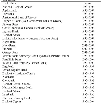
While the number of commercial banks operating in the Greek banking system
remained almost unchanged since 1993, the number of those banks’ branches and
employees has increased significantly (see Table 1). During this period, a number of new,
mainly small, commercial banks opened and a series of mergers and acquisitions were
16
The indirect control comes from the majority equity participation of public pension funds, municipalities and other funds, or from equity holdings of other state-owned or state-controlled banks.
17
undertaken, altering the level of bank concentration and substantially changing the structure
of the Greek banking system. Specifically, especially during the first half of the 1990s, new
private-owned foreign commercial banks were established, taking advantage of new
products and services that were not available in the Greek market just a decade ago. Later
on, other Greek commercial banks were established, primarily focusing on retail banking.
Moreover, since the mid 1990s, several Greek banks have been involved into mergers and
acquisitions, in order to become more efficient and obtain a size that would enable them
to increase or, at least, maintain their domestic market shares, facilitate their access to
international financial markets, and exploit any possible economies of scale. Most of
them concerned the domestic market, including not only banks but also non-bank
financial enterprises. Some large credit institutions opted to merge with their subsidiaries
with a view to restructuring their activities and cutting back on their operating expenses.
These mergers and acquisitions have reversed the downward trend observed in
bank concentration during the previous decade. The market share of the 5 largest credit
institutions reached 65 per cent in terms of balance sheet aggregates in 2004 (being in
similar and higher levels in the period 2001-2003), up from 57 per cent in 1997 (Bank of
Greece, 2006). Similar are the conclusions if we use the Herfindahl-Hirschman Index
(HHI).18 Its value stands at 1,069 in 2004, up from 885 in 1997. In any case, both
concentration ratios characterizing the Greek banking sector are much higher than the
average European levels (the share of the 5 largest credit institutions stands, on average,
at 40 per cent, while the HHI index reaches 569 in 2004) (European Central Bank, 2004,
2005).
18
Even though the Greek banking system is characterized by a relatively high degree
of market concentration, the five larger Greek commercial banks would be classified as
mid-size by European standards; only the first two banks are included among the top 100
European banks, while none in the top 150 credit institutions at a global level (Bank of
Greece, 2005). This is principally due to the limited size of the domestic credit market and
the absence of significant presence abroad.
To compete in the new financial landscape and strengthen their position in the
market, Greek commercial banks are transforming themselves into financial groups, (i)
adding subsidiaries such as insurance companies, brokerages, credit card companies,
mutual fund firms, factoring companies and finance houses, so as to offer additional
services, and (ii) expanding their activities abroad, principally to the South Eastern
European region (Albania, Bulgaria, Former Yugoslav Republic of Macedonia, Romania,
Serbia and Montenegro, and recently Turkey), via subsidiaries or through the
establishment of branches. This latter trend signifies that Greek banks in the region have
some comparative advantage, in the form either of access to capital markets, or of superior
organization, know-how, and good understanding of local conditions.
The above-mentioned developments in the structure of the Greek banking system
resulted in significant modifications in the balance sheet and profit and loss accounts.
More notably, the ratio of net interest income to average total assets (i.e. the net interest
margin) of Greek commercial banks increased considerably during the examined period,
raising from 1.57 per cent in 1993 to 2.80 per cent in 2004.19 Also, the proportion of
19
loans to total assets reached 63 per cent at 2004 (compared to 24 per cent in 1993),
catching up rapidly with the average European levels.20
The high proportion of operating expenses is related to the specific features of the
Greek banking system, such as the high number of branches of large banks and the fact that
the products offered are relatively limited (Hondroyiannis et al., 1999). However, although
Greek banks' operating expenses relative to their average total assets remain above the
average European figures, they fell from 2.9 per cent to 2.3 per cent between 1996 and
2004. During this period, Greek credit institutions took important steps towards improving
their efficiency by deploying modern information technology systems, cutting down on
their operating costs and improving their organizational structure, while extending their
scope of business by offering new products and services. Finally, Greek banks have
increased their levels of loan loss provisions, mainly by reason of the significant credit
expansion. Taking into account these developments, indications of a long-term downward
trend in profitability will be observed, evident from the beginning of liberalization (towards
the end of the 1980s) onwards (Gibson, 2005).
4.2. Data
The models specified above are used in order to examine the level of competition
in the Greek banking industry during the period 1993-2004. All bank-level data are taken
from Balance Sheet Accounts and Income Statements published annually by the Greek
20
banks included in the sample. The macroeconomic data (national income and Greek
Treasury bond rates) were drawn from Eurostat and the Bank of Greece.
Our sample covers all Greek commercial banks, plus a foreign-owned credit
institution, namely Bank of Cyprus. The institutions that do not publish profit and loss
statements, i.e. branches of foreign banks and certain specialized credit institutions, are
not included in the sample.21 Specialized credit institutions and smaller cooperative banks
are also excluded from the analysis, since (i) their operations differ substantially from those
of the mainstream commercial banks and (ii) sometimes they have a different legal form.
Last, we omit investment banks and banks focusing in corporate banking, since they fail to
meet the criterion of being a well-rounded commercial banking institution (universal credit
institution). The number of credit institutions included in the sample ranges from 13 to 23
commercial banks in each year of the examined period (see Table 2). In all examined
years, the banks included in the sample accounted for a significant proportion of total
banking assets (around 80 per cent).
The output variable in the CPM (namely Q when referring to the industry’s total
output and q when referring to the individual bank’s output) is defined as the value of
total bank assets in real terms (in million euros). The unit price of output (namely P at the
market level and p at the bank level) is measured as interest income over total assets. The
choice of cost, price and output variables follows either the intermediation or the
production approach. According to the intermediation approach, banks are considered as
financial intermediaries that combine deposits together with purchased inputs to produce
bank assets. Total cost includes interest expenses and operating expenses, i.e. staff costs
21
and administrative expenses. In the alternative production approach, banks utilize capital
and labor inputs to produce outputs of loans and deposit accounts. In this paper we follow
the intermediation approach. The three input variables are defined as follows:
Labor (L): Defined as total number of employees.
Physical capital (K): Defined as fixed assets, including tangible fixed assets (land,
lots, buildings and installations, furniture, office equipment, etc., less depreciation), as
well as intangible fixed assets (goodwill, software, restructuring expenses, research
and development expenses, minority interests, formation expenses, underwriting
expenses, etc).
Total intermediated funds (F): Include current accounts, savings accounts, time
deposits, repurchase agreements, as well as alternative funding sources (e.g. retail
bonds).
The unit prices of the three respective inputs (w1, w2, and w3)are defined as follows:
Unit price of labor (w1): Ratio of personnel expenses to total labor. Personnel
expenses include wages and salaries, social security contributions, contributions to
pension funds, and other staff-related expenses.
Unit price of funds (w2): Ratio of interest expenses to total funds. Interest expenses
include interest paid on deposits and other sources of funds.
Unit price of physical capital (w3): Ratio of administrative expenses to fixed assets.
Administrative expenses include rents, service charges, security, information systems
and communications, other office and insurance expenses, professional charges,
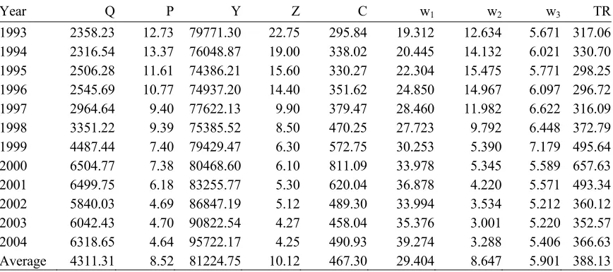
Finally, regarding the RT, TR stands for real total revenue (this refers to real total operating
income, which includes interest income, dividend income, fee and commission income,
gains less losses from securities, and other operating income). In Table 3 we report banking
indicators of the variables described above for the period 1993-2004.
5. Empirical results
In Tables 4-7 we present the empirical results of the static and dynamic CPM and
RT. There are four pairs of columns in each table. In the first, we provide the results of the
basic models, as described in Section 4. In the second, the real variables are replaced by
nominal ones (in order to be consistent with the part of the literature that uses nominal
variables), while in the third we include a quadratic time trend, to capture any trends in
output prices and revenues in the CPM and RT, respectively. Finally, in the fourth pair of
columns, we add time dummies for all years (time fixed effects), thus modifying the model
to a three-way error component (see Baltagi, 2005). The time dummy specification is more
general than the linear trend specification, as it will pick up potential trends of the variables
used and more complex bank-level patterns.22 All these modifications are applied on a
one-by-one basis and not in a cumulative manner; so, for example, the modified model
containing time dummies for every year does not also contain a trend, and the amounts it
uses are real. The lag length in the dynamic models is set to one, which rejects
autocorrelation; hence higher order autocorrelation is not accounted for in the regressions
(this is expected given the fact that the data are annual).
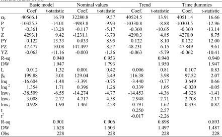
The results obtained by running the 3SLS estimation procedure on System (6) are
presented in Table 4. The R-square statistics of both demand and supply relations, ranging
from 0.89 to 0.96, indicate fine goodness of fit. The Durbin-Watson (DW) statistic reveals
possible autocorrelation in the supply equation, which is a common problem in the
literature (see Toolsema, 2002), whereas the DW statistic of the demand equation
surprisingly rejects the hypothesis of serial correlation. All parameters of the demand
relation were found to be statistically significant, which is a crucial factor in the
identification of L (except the intercorrelation variable YZ when nominal amounts are
used). In particular, the coefficient on P is negative and statistically significant, meaning
that the demand function is decreasing in its own price, as expected. The negative sign on Y
suggests that income refers to the ability to pay for the goods bought with consumer credit,
in the sense that high income may imply less need for such credit (Toolsema, 2002). On the
other hand the coefficient of the Greek government bond yield (Z) is positive and
statistically significant, implying that our choice of Z is well suited as the price of a
substitute.
In the supply equation, the parameters were not all statistically significant, which
may be due to the dynamic nature of output and inputs in banking (especially when we
include time dummies most t-statistics decrease). The coefficient on the unit price of labor
contrasts our expectations, a fact that may be due to the labor surplus in the beginning of
the period examined and the gradual reduction in labor expenses by Greek banks in order to
improve their operating efficiency. In contrast, the coefficients of the other two inputs have
the expected sign.
22
The estimate of market power, L, is very close to zero in all cases and the
corresponding t-statistics are small, indicating that L is not significantly different from zero.
Thus, the static CPM analysis specifies that the Greek banking market is characterized by
perfect competition. This means that the high degree of concentration characterizing the
Greek banking industry reflects the efforts by the most efficient banks to take advantage of
economies of scale and scope and does not necessarily influence competition in a negative
manner. This conclusion is different from the results of studies of market power in
banking sectors of several European countries, which generally find evidence of
monopolistic competition or collusive conduct.
5.2. Dynamic CPM
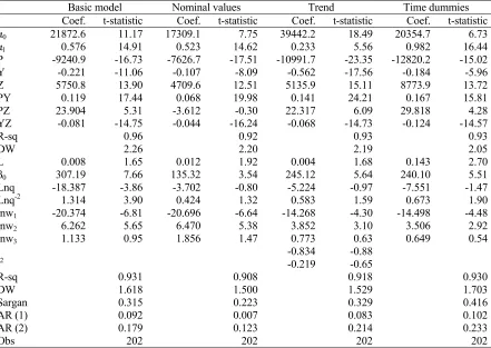
The results obtained by examining the dynamic CPM are presented in Table 5.
Once again, as in the static model, the parameters in the demand equation are strongly
statistically significant at the 5 per cent level of significance, the only exception being the
coefficient of the cross-term PZ when nominal values are applied. The R-squarestatistic of
the supply relation attains values slightly higher compared to that of the static CPM, which
indicates that the dynamic model contains somewhat more information, especially for input
prices. The Durbin-Watson statistic is also improved, verifying that the autocorrelated
errors can be made to disappear by incorporating additional dynamics; as Kennedy (2003)
states, modern econometric models typically have a rich dynamic structure and only
seldom involve autocorrelated errors. The signs of the estimated coefficients are
unchanged; however the t-statistics of both bank output and inputs (especially for w2) are
The estimate of market power, L, is positive and close to zero (yet with a
significantly higher t-statistic), except the one from the specification that includes time
dummies. In the latter case, L is statistically significant at the 5 per cent level of
significance. This is a striking result since we cannot accept the interpretation of perfect
competition as in the static CPM, meaning that some form of collusive behavior
characterizes the Greek banking sector.23 Such an outcome may imply that the dynamics
inherent in the use of bank-level data mask – to some extent – the market power exercised
in the industry, a result effectively towards the same direction with the theoretical
considerations of Corts (1999). To this end a dynamic CPM model may be a more
appropriate specification.
5.3. Static RT
The competitive position tests of the static RT are presented in Table 6. In all
models we include time dummies for the years 1999 and 2000 to account for the
exceptional developments in the Greek stock market that took place during this period and
led to a boom in bank revenues. The R-square statistic in all four estimated equations,
ranging from 0.97 to 0.98, indicates fine goodness of fit. The coefficients on w1 and w3 are
reported with the expected positive sign and they are statistically significant only when the
trend or the time dummies are included in the specifications, a fact that provides evidence
of improved stability of the equations. The coefficients on w2 and TA are always positive
and statistically significant.
23
The value of the H-statistic ranges from 0.214 (basic specification) to 0.605 (when
time dummies are incorporated), and in all cases is statistically significant. The Wald test
reveals that the H-statistic differs significantly from both zero and unity and, therefore, the
hypotheses of both monopoly and perfect competition are rejected. Given the discussion in
Sections 2 and 3, the dominant market form suggested by the static RT is monopolistic
competition. Finally, we test for long-run equilibrium using the return on assets as the
dependent variable. The Wald test performed does not reject the hypothesis of equilibrium
(Hn = 0) at conventional statistical levels (x2 (4) = 52.93, p-value = 0.000), which implies
that our analysis is well specified.
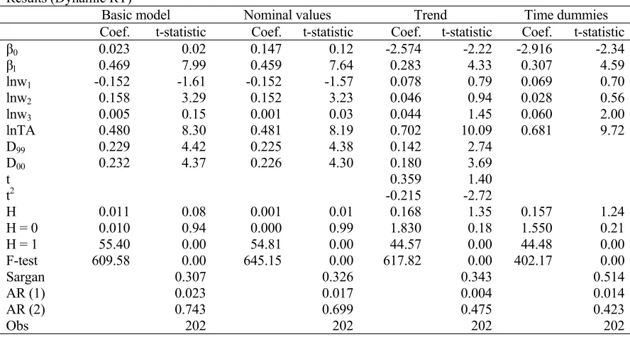
5.4. Dynamic RT
Table 7 presents the results of the dynamic RT model (Eq. 10). In this specification,
the significance of the input prices falls compared to the static RT (only the coefficient on
w2 is positive and statistically significant in the basic model and when nominal values are
applied and the coefficient on w3 when time dummies are included in the specification).
The effect of TA remains positive and statistically significant, TA attaining however lower
values compared with the static RT.
More importantly, we note that the value of the H-statistic is practically
indistinguishable from zero in the cases of the basic model and its variant with nominal
values, whereas in the models where time-related terms are added, either in the form of a
time trend or in the form of time dummies, H departs from zero, attaining values around
0.16. The hypothesis tests H = 1 and H = 0 show that perfect competition is rejected for
respectively (at the 5 per cent level of significance). The test for examining the existence of
long-run equilibrium once again confirms the hypothesis of equilibrium at the 5 per cent
level, even though the Wald test attains a lower value compared to the static case (x2 (4) =
16.08, p-value = 0.003). 24
The signs found are consistent with the view that the CPM and RT offer similar
conclusions regarding the structure of the Greek banking sector. Yet, both dynamic models
indicate at least some anticompetitive behavior of banks, while their static counterparts
point towards competitive conduct. These results have noteworthy implications for
researchers and policy makers, as they challenge the dominant arguments regarding the
structure of the Greek banking sector. One could elicit further information if these models
were compared to a variety of differently structured banking systems or if they were
extended to account for the critiques of the NEIO literature (e.g. Corts, 1999). Yet, before
we move on to another issue we had better bring this entry to a close.
6. Concluding remarks
Contrary to standard accounts, we have used both a CPM and a RT to assess
competitive conditions in a specific banking industry. The analysis further distinguished
between static and dynamic versions of these models in order to substantiate whether
predictions regarding the market structure remained unchanged. We tested the four
24
resulting specifications, using panel data from the Greek banking industry over the period
1993-2004.
We contend that our results indicate that both static models tend to underestimate
the level of market power. In particular, while the static CPM and RT indicate no
anticompetitive conduct and monopolistic competition respectively, their dynamic
counterparts signal some anticompetitive behavior of banks. This is especially true for the
dynamic RT, and for the dynamic CPM when time dummy variables are included in its
empirical specification. We may partially attribute the mask of market power by static
models to the important dynamics that characterized the Greek banking sector during the
examined period, which were not reflected in the empirical specifications of either the
static CPM or the static RT. These results hold consistently across a number of econometric
specifications and estimation methods, as applied separately to the static and dynamic
models, enhancing some recent critiques regarding the suitability of static NEIO models to
robustly estimate market power.
At a broader level of analysis the conclusions of the present article underline the
crucial relevance of the special features of the examined banking industry and they
highlight the need to develop more appropriate empirical methodologies to characterize the
References
Amemiya, T., 1977. The maximum likelihood estimator and the nonlinear three-stage least
squares estimator in the General Nonlinear Simultaneous Equation Model.
Econometrica 45, 955-968.
Arellano, M., Bond, S., 1991. Some tests of specification for panel data: Monte Carlo
evidence and an application to employment equations. Review of Economic Studies 58,
277-297.
Arellano, M., Bover, O., 1995. Another look at the instrumental variables estimation of
error-component models. Journal of Econometrics 68, 29-51.
Baltagi, B., 2005. Econometric Analysis of Panel Data, 3rd edition. John Wiley & Sons,
Chichester.
Bank of Greece, 2005. Annual Report for 2004. Bank of Greece (in Greek).
Bank of Greece, 2006. Annual Report for 2005. Bank of Greece (in Greek).
Barajas, A., Steiner, R., Salazar, N., 2000. The impact of liberalization and foreign
investment in Colombia’s financial sector. Journal of Development Economics 63,
157-196.
Barnett, W.A., Lee, Y.W., 1985. The global properties of the Minflex Laurent,
Generalized Leontief and translog flexible functional forms. Econometrica 53,
1421-1438.
Berger, A, Bonime, S., Covitz, D., Hancock, D., 2000. Why are bank profits so persistent?
The roles of product market competition, informational opacity, and
Bikker, J., Haaf, K., 2002. Competition, concentration and their relationship: An empirical
analysis of the banking industry. Journal of Banking and Finance 26, 2191-2214.
Binder, M., Hsiao, C., Pesaran, H., 2003. Estimation and inference in short panel vector
autoregressions with unit roots and cointegration, Mimeo.
Blundell, R., Bond, S., 1998. Initial conditions and moment restrictions in dynamic panel
data models. Journal of Econometrics 87, 115-143.
Bond, S., 2002. Dynamic panel data models: A guide to microdata methods and practice.
Portuguese Economic Journal 1, 141-162.
Bourke, P., 1989. Concentration and other determinants of bank profitability in Europe,
North America and Australia. Journal of Banking and Finance 13, 65-79.
Bresnahan, T., 1982. The oligopoly solution concept is identified. Economics Letters 10,
87-92.
Bresnahan, T., 1989. Empirical studies of industries with market power. Chapter 17 in
Handbook of Industrial Organization (editors: Richard Schmalensee, Robert Willig),
Vol. 2, Elsevier Science Publications, 1011-1057.
Carlton, D., Perloff, J., 2005. Modern Industrial Organization. Addison-Wesley, 4th Edition.
Corts, K.S., 1999. Conduct parameters and the measurement of market power. Journal of
Econometrics 88, 227-250.
De Bandt, O., Davis, P., 2000. Competition, contestability and market structure in
European banking sectors on the eve of EMU. Journal of Banking and Finance 24,
1045-1066.
European Central Bank, 2004. Report on EU banking structure. European Central Bank,
European Central Bank, 2005. Banking structures in the new EU member states. European
Central Bank, January.
Evanoff, D., Fortier, D., 1988. Re-evaluation of the structure-conduct-performance
paradigm in banking. Journal of Financial Service Research 1, 277-294.
Gibson, H., 2005. Greek banking profitability: Recent developments. Bank of Greece,
Economic Bulletin 24, 7-26.
Hansen, L., 1982. Large sample properties of generalized method of moments estimators.
Econometrica 50, 1029-1054.
Hondroyiannis, G., Lolos, S., Papapetrou, E., 1999. Assessing competitive conditions in the
Greek banking system. Journal of International Financial Markets, Institutions and
Money 9, 377-391.
Hughes, J.P., Mester, L.J., 1998. Bank capitalization and cost: Evidence of scale economies
in risk management and signaling. Review of Economics and Statistics 80, 314-325.
Iwata, G., 1974. Measurement of conjectural variations in oligopoly. Econometrica 42,
947-966.
Kennedy, P., 2003. A Guide to Econometrics, fifth edition. Blackwell Publishers, Oxford.
Lau, L., 1982. On identifying the degree of competitiveness from industry price and output
data. Economics Letters 10, 93-99.
Ljung, G., Box, G., 1979. On measure of lack of fit in time series models. Biometrika 66,
265-270.
Molyneux, P., Lloyd-Williams, M., Thornton, J., 1996. Competition and market
contestability in Japanese commercial banking. Journal of Economics and Business 48,