Extracting the Cyclical Component in Hours Worked: a Bayesian Approach

Munich Personal RePEc Archive

Extracting the Cyclical Component in

Hours Worked: a Bayesian Approach

Bernardi, Mauro and Della Corte, Giuseppe and Proietti,

Tommaso

University of Rome, Tor Vergata

May 2008

Online at

https://mpra.ub.uni-muenchen.de/8967/

Extracting the Cyclical Component in Hours

Worked: a Bayesian Approach

Mauro Bernardi

Giuseppe della Corte

Tommaso Proietti

Dipartimento S.E.F. e ME.Q., Via Columbia 2, 00133 Roma, Italy.

Abstract

The series on average hours worked in the manufacturing sector is a key leading indicator of the U.S. business cycle. The paper deals with robust estimation of the cyclical component for the seasonally adjusted time series. This is achieved by an unobserved components model featuring an irregular component that is represented by a Gaussian mixture with two components. The mixture aims at capturing the kurtosis which characterizes the data. After presenting a Gibbs sampling scheme, we illustrate that the Gaussian mixture model provides a satisfactory representation of the data, allowing for the robust estimation of the cyclical component of per capita hours worked. Another important piece of evidence is that the outlying observations are not scattered randomly throughout the sample, but have a distinctive seasonal pattern. Therefore, seasonal adjustment plays a role. We finally show that, if a flexible seasonal model is adopted for the unadjusted series, the level of outlier contamination is drastically reduced.

Keywords: Gaussian Mixtures. Robust signal extraction. State Space Models. Bayesian model selection. Seasonality.

1

Introduction

The series of average weekly hours in manufacturing (AWH, henceforth) is an im-portant indicator of the state of the U.S. economy. It is considered, in particular, a leading economic indicator of output and employment in manufacturing (see for in-stance Glosser and Golden, 1998), since firms usually tend to respond to business cycle conditions by decreasing or increasing hours worked, before hiring or laying off workers. According to Cho and Cooley (1994), a sizeable share of the adjustment in total hours over the business cycle represents adjustment in average hours, while the remainder concerns changes in employment. Also, the procyclicality of per capita hours worked and their response to technology shocks is the subject of a vivid ongoing debate, see Gal´ı and Rabanal (2005) and the references therein. Finally, AWH is listed among the 10 indicators that make up the Conference Board composite index of leading indicators (CBO, 2001).

The series measures an average of the number of hours worked per week by produc-tion workers in U.S. manufacturing industries. It is produced by the U. S. Bureau of Labor Statistics (http://www.bls.gov/ces/), as part of the Current Employment Statis-tics (CES) monthly survey, which obtains payroll hours, employment and earnings from business establishments.

The series is usually analyzed in seasonally adjusted (SA) form. Seasonal adjust-ment is carried out by the BLS according to the methodology reported at http://www-.bls.gov/ces/cesseasadj.htm. A particular problem is posed by the treatment of calen-dar related fluctuations, and in particular by the treatment of moving festivals (Easter and Labor day). As a matter of facts, the data are collected from the respondents’ payroll records for the pay period that includes the 12th of each month. Thus, if Easter or Labor day falls during the week including the 12th, the number of hours worked will be reduced.

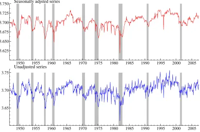
The seasonally adjusted series is plotted in the top panel of figure 1; the super-imposed shaded ares locate the NBER recessions. The plot confirms the tendency to lead the business cycle peaks, and reveals the presence of a few occasional large drops in hours worked. The standardized fourth moment of the monthly growth rates is equal to 22.5, and the Jarque-Bera (JB, 1980) normality test statistics for this series is 11518. When computed on the yearly growth rates, the kurtosis drops to 3.79, and the JB normality statistics is a mere, though significant, 18.9. The unadjusted series is presented in the bottom plot. A noticeable feature is that the seasonal component does not look regular and evolves over time. It is perhaps interesting to single out the period 1975-1980, when the SA series is characterized by the same troughs as the unadjusted series.

finite mixtures provide a flexible tool to model outliers and skewed distribution. Outlying observations and structural breaks in the components can be handled by the inclusion of appropriate dummy variables on the right hand side of the measurement and transition equations. However, this strategy has several drawbacks: for instance, when a dummy is used to capture an additive outlier, this amounts to considering the corresponding observation as missing, so that a weight of zero is assigned to it in signal extraction and forecasting; on the contrary, the observation may still contain some information, which could be elicited by suitable downweighting. An alternative strategy consists in allowing the disturbances of a structural model to possess a heavy tailed density, such as Students’ t-distribution, the general error distribution (Durbin and Koopman, 1997), or a mixture of Gaussian (Harrison and Stevens, 1976, Fr¨ uhwirth-Schnatter, 2006, Giordani, Kohn and van Dijk, 2007). The second strategy is preferred in this paper since it allows to single out which observations are outlying.

The unobserved components model Gaussian mixture model provides a good fit to the data and is a significant improvement over a standard linear model, as it is revealed by model selection according to a proposal by Chib and Jeliazkov (2001).

The paper is structured as follows. Section 2 presents the unobserved components model for the seasonally adjusted series. Bayesian inference is discussed in section 3, whereas section 4 addresses the issue of model selection and deals with the estimation of the marginal likelihood of our model, using the approach suggested by Chib and Jeliazkov (2001). In section 5 we presents and discuss the estimation results, which finally lead us to the specification and the estimation of an unobserved components Gaussian mixture model for the unadjusted series (section 6). Section 7 concludes the paper.

2

The Gaussian mixture model

Let ySA

t , t = 1, . . . , n, denote the logarithm of seasonally adjusted AWH. The model

for the series, plotted in the upper panel of figure 1, is an additive decomposition into a trend component, µt, representing the underlying long run evolution of the series, a

stationary cycle, ψt, and an irregular component,ǫt, which is specified as follows:

ySA

t = µt+ψt+ǫt,

µt = µt−1+ηt, ηt∼N(0, ση2),

ψt = φ1ψt−1+φ2ψt−2+κt, κt∼N(0, σ2κ)

ǫt = (1−St)ǫ0t+Stǫ1t ǫit∼N(0, σǫi2),

St ∼ IID Bernoulli(ω)

(1)

The trend is a random walk, whereas the cycle is an autoregressive process of order 2, AR(2), with stationary complex roots, which is achieved via the reparameterization in terms of the modulus and the phase of the roots of the AR polynomial. In particular, we writeφ1 = 2ρcosλc and φ2 =−ρ2, where ρ is defined in the interval (0,1), and λc

We assume that the irregular component has a finite mixture distribution, with two components. Denoting byf(ǫt) the probability density function ofǫtand byg(ǫt;µ, σ2ǫ)

the univariate Gaussian density with meanµ and varianceσ_ǫ2,

f(ǫt) = (1−ω)g(ǫt; 0, σǫ20) +ωg(ǫt; 0, σ2ǫ1). (2)

We identify the mixture parameters by imposing the ordering restriction σ2

ǫ0 < σ2ǫ1.

LettingSt denote an IID Bernoulli indicator variable taking the values 0,1 with

prob-ability ω = P(St = 1) and 1−ω = P(St = 0), respectively, when the series is in a

low volatility state 0, the irregular variance isσ2

ǫ0;σ2ǫ1 is the irregular variance in the

high volatility state (St= 1). This identification constraint avoids the label switching

problem; see Geweke (2005) and Fr¨uhwirth-Schnatter (2006) for details.

We further assume that the random disturbances ηt, κt, ǫ0t, ǫ1t are mutually

inde-pendent. Conditionally on St, the model (1) is a linear Gaussian state space model

with measurement equation given by the first equation and transition equation built from the Markovian representation forµt and ψt.

3

Bayesian Estimation

In this section we discuss how we make inference for the model presented in section 2. In particular, we discuss our prior choices, and we describe the algorithm used for computing the posterior distribution and the full conditional distributions.

Let x={µt, ψt, t= 0, . . . , n} denote the collection of the unobserved components,

Ψ = (ση2, σκ2, σǫ20, σ2ǫ1, λc, ρ, ω) the vector of parameters of the model as defined in section

2. We further denote byS ={S1, . . . , St, . . . , Sn}then−dimensional vector of indicator

variables St.

Our objective is to estimate the parameters of the posterior distribution of the vector of parameters Ψ, of the the unobserved states and the latent indicator, by generating random draws from the joint posterior of the unobserved components and vector of parameters itself, p(Ψ, S, x|y), where y = ¡ySA

1 , ySA2 , . . . , ynSA

¢

denotes the vector of seasonally adjusted observations. A Metropolis-Hastings within Gibbs sam-pling algorithm is implemented, where we take the vectorS, the matrix of unobserved states as a single block and partition the vector Ψ into three blocks, Ψ = (Σ′_,Λ′_{, ω)}′_,

where Σ =¡σ2_η, σ2_κ, σ2_ǫ0, σ_ǫ2₁¢, Λ = (λc, ρ), andω is the mixing probability.

3.1

Prior Distributions

Table 1: Prior hyper-parameters, initial values of the chain and lower bounds.

Parameter Initial Value α0_J β_J0 Lower Bound

σ2

η 2.83E-07 4.0 5.67E-07 1.00E-010

σ2_κ 3.66E-04 4.0 7.32E-04 1.00E-06

σ2

ǫ0 4.83E-06 4.0 9.67E-06 1.00E-07

σ2_ǫ1 4.83E-05 4.0 9.67E-05

-The usual Inverted Gamma prior distribution is chosen for the scale parameters in Σ, while a Beta distribution is chosen for the cycle parameters (λc, ρ), and for the mixing

probabilityω. This gives rise to the following structure of prior distributions:

p(Σ,Λ, ω)∝p(Σ)p(Λ)p(ω) (3)

where we assume an independent structure between each block of variables and within each block

p(Σ) ∝ Y

J

IG

µ

σ2J,

α0

J

2 ,

β0

J

2

¶

, ∀J ={ǫ0, ǫ1, η, κ} (4)

p(Λ) ∝ Be¡ρ|p0₁, p0₂¢×πBe¡λc|c01, c02 ¢

I[0,π] (5)

p(ω) ∝ Be¡ω|s0₁, s0₂¢. (6)

The choice of an inverted gamma structure for the variance parameters in Σ is motivated by the aforementioned need of avoiding improperness of the posterior dis-tributions in the mixture framework. Under these priors the variance parameters have independent inverted gamma conditional posteriors, even in the case on no observa-tions allocated to one of the two mixture components. However, as pointed out by Harvey, Trimbur and van Dijk (2007), the use of very slow shape and scale parameters for these distributions may lead to problems in estimation, in particular for parameters that tend to take on small values such as the variance of the trend component. In order to avoid distortions in the estimates of the variance components and degeneracy of the sampler, we introduced the lower bounds reproduced in the last column of table 1, even if in the post-processing of the simulations we realize that these bounds are not binding most of the time. The choice of a uniform prior for the cycle parameters (ρ, λc), over

the stationarity region, which is a bounded region inR×R, i.e. (ρ, λc)∈(0,1)×[0, π],

does not pose a problem in terms of successfully generating competitive parameter values. As described in section 3.3 above, we use a Metropolis step for the simulation of variate from this full conditional distribution.

3.2

Likelihood and posterior

The complete-data likelihood is

p(y, x, S|Ψ) =

n

Y

t=1

where

p(yt|xt, St,Ψ) =

©

ωg¡yt|xt, St= 0, σǫ20

¢ ª1−St©

(1−ω)g¡yt|xt, St= 1, σ2ǫ1 ¢ ªSt

, (8)

represents the density of the mixture,p(xt|xt−1,Ψ) is the transition density of the state

space model which is markovian for the representation of the unobserved components proposed we use here, (see, e.g. Harvey, 1989), and p(x0) is the prior distribution

on the initial vector of states x0, which is diffuse for non-stationary components and

centered around the long-term mean for the stationary component. The joint posterior distribution of the parameters and the unobservable components,p(Ψ, x, S|y) will be proportional to the product of the likelihood and the prior distributions given in the previous subsection.

3.3

The Gibbs sampler

The Gibbs sampling approach to estimating the model parameters involves sampling from the complete conditional distribution of each parameter in a systematic manner, conditional on the previous sampled values of the other parameters. This approach is always possible, since the complete conditional densities are available, up to a normal-izing constant, from the form of the likelihood and the prior (see, Geman and Geman (1994), and de Pooter, Segers and Van Dijk (2006) for an up to date overview of the state of the art in Bayesian computation using Gibbs sampler). When some of these conditional densities do not have standard form, as is often the case, the Metropolis-Hastings algorithm may be used to obtain realizations from a Markov chain having the required stationary distribution (see e.g., Casella and Robert (2004), and Gamerman and Lopes (2007)).

After choosing a set of initial values for the parameter vector Ψ(0), simulations

©

Ψ(i)_{, x}(i)_{, S}(i)ª_{, i= 1,2, . . ., from the posterior distribution are obtained by iterating}

the following steps of the Gibbs sampler.

(i) Update the indicator variable

p(St= 1|Ψ(i), x(i), y) ∝

ω σǫ0

exp

½

− 1

2σ2

ǫ0

(yt−µt−ψt)2

¾

+(1−ω)

σǫ1

exp

½

− 1

2σ2

ǫ1

(yt−µt−ψt)2

¾

(9)

with t= 1, . . . , n.

(ii) Simulate the matrix of unobserved componentsx(i+1), from the complete full con-ditional distribution p(x|Ψ(i)_{, S}(i+1)_{, y), where S}(i+1) _{is the vector of indicator}

variables generate at the previous step of the Gibbs sampler.

(iii) Simulate the cycle parameters (ρ, λc)(i+1) from the full conditional distributions

p³ρ|λ(_ci),Σ(i), ω(i), x(i+1), S(i+1), y´∝p(ρ)

×exp

(

1 2σ2

κ n

X

t=1 ¡

ψt−ρcosλcψt−1+ρ2ψt−2¢2 )

and

p³λc|ρ(i+1),Σ(i), ω(i), x(i+1), S(i+1), y

´

∝p(λc)

×exp

(

1 2σ2

κ n

X

t=1 ¡

ψt−ρcosλcψt−1+ρ2ψt−2 ¢2)

, (11)

where ψt, t = 0,1, . . . , n, is defined as ψt = yt−µt, and the prior distributions

are beta, as described in the previous section.

(iv) Simulate Σ(i+1) _{from the complete full conditional distributions}

p³σJ2|Λ(i+1), x(i+1), S(i+1), y

´

∝ IG¡σJ2|αJ, βJ

¢

, ∀J ={ǫ0, ǫ1, η, κ}. (12)

The parameters of these posterior distributions are

αJ =

α0

J

2 +

nǫJ

2 , βJ =

β0 J 2 + ¯ SJ 2 ,

where forJ ={ǫ0, ǫ1},nǫ0 = Pn

t=1Standnǫ1 = Pn

t=1(1−St)are are the number

of observations allocated to the two components of the mixture,

¯

Sǫ0 =

n

X

i=1

St(yt−µt−ψt)2, S¯ǫ1 =

n

X

i=1

(1−St) (yt−µt−ψt)2,

and, for the trend and cycle posterior variance, J ={η, κ}, we have αJ = a

0

J+n

2 ,

and

βη =

α0 η 2 + 1 2 n X t=1

(µt−µt−1)2

βκ =

α0 κ 2 + 1 2 n X t=2 ¡

ψt−ρcosλcψt−1−ρ2ψt−2¢2.

(v) Simulate the mixing probabilityω(i+1), from the complete full conditional distribu-tion

p³ω|Λ(i+1), β(i+1),Σ(i+1), S(i+1), S(i+1), y´∝ Be(ω|g0+nǫ0, h0+nǫ1). (13)

We generate random draws from the full conditional distribution of the statesp(x|Ψ, S, y), at point (ii), using the simulation smoother for a linear state space model, developed by de Jong and Shephard, (1996) and Durbin and Koopman (2001)). All the compu-tations are carried out in Ox 4.10 by Doornik (2006). For the simulation smoother we use the library Ssfpack, version 2.3, see Koopman et al. (1999).

The conditional posterior distributions of the cycle parameters (ρ, λc), at point

Metropolis et al. (1953) and Hastings (1970)) steps where the candidate distributions are chosen to have the same supports than the conditional posteriors and the variances can be calibrated using a small number of iterations of the algorithm in order to have an acceptance ratio of about 50%. More specifically, in order to sample from the full conditional posterior of ρ(i), for example, we generate candidate values from a Beta distribution, Be(a, b), where we pose the mean of the Beta distribution to be equal to the previously generated value of the parameter ρ(i−1)_{. By inverting the relation}

linking the mean and the variance of the Beta distribution to its parameters (a, b), we obtain the following relation

(

a= ρ2i₋1(1−ρi−1)−v ρi−1

v

b=a1−ρi−1

ρi₋1

whereρi−1 is the value generated by the Metropolis-Hastings sub-chain at step (i−1)

and v is the variance of the proposal distribution. This parameters choice allows us also to avoid numerical problems related to the evaluation of the Metropolis-Hastings acceptance ratio in the presence of fat tailed and quite spiked likelihood functions. We carry out the same operations for the parameterλc.

4

Model Selection

In this section, we give a brief account of Chib and Jeliazkov (2001) method to calculate an estimate of the marginal density using the output from the Metropolis-Hastings algorithm. This methodology allows us to discriminate which model, amonggdifferent proposals, provides a better representation of a vector a data y = (y1, y2, . . . , yn), in

an appropriate statistical sense. Euristically, we want to compare how likely are the data under the gdifferent models, integrating over the parameter space.

Let us denote by p(y|Ψk,Mk) the density function of the data under model Mk

and a vector of parameters, Ψk, and p(Ψk|Mk) as the prior density. In this paper,

we compare two different modelsMk: M1 is a standard Gaussian state space model

where the structural components are trend and cycle, whileM2 is the Gaussian

mix-ture model defined in equation 1. These models differ for the treatment of the error component, which is a standard Gaussian distribution in M1, and a mixture of two

normal distribution inM2. Since the two components of the mixture distribution have

the same mean but different variances, the implied unconditional distribution exhibits fatter tails than in the normal case. The marginal density of the data under model

Mk is

m(y|Mk) =

Z

p(y|Ψk,Mk)p(Ψk,Mk) dΨk, k= 1,2, (14)

where p(Ψk,Mk) represents the prior distribution of the parameter vector Ψk under

modelMk. The formal bayesian approach for comparing modelM1andM2is through

the pairwise Bayes factor, defined as the ratio of marginal likelihoods

B1,2 =

m(y|M1)

m(y|M2)

which can also be interpreted as the posterior probability of model M1, when both

models are, a priori, equally likely. For a exhaustive discussion on Bayesian model comparison using Bayes factors, we refer to the paper of Kass and Raftery (1995), Chipman et al. (2001), Pericchi (2005) and the bibliography quoted therein, in partic-ular for the explanation of why it may be misleading to use arbitrary vague priors and improper priors in a model selection framework.

Calculating the marginal density, and hence the Bayes factor, is a daunting task when estimation of the unknown parameters has been done by Markov chain Monte Carlo methods. Recently, several Monte Carlo methods for computing the marginal likelihoods have been developed, which include the Chib estimator, Chib (1995), the ratio of importance sampling, Chen and Shao (1997), the path sampling, Gelman and Meng (1998), the bridge sampling, Meng and Shilling (2002), and the extension of the Chib (1995) estimator for the case of some Metropolis steps within the Gibbs sampler, Chib and Jeliazkov (2001). In what follows we adapt the Chib and Jeliazkov (2001) method to our general framework, in which some blocks of parameters of the posterior distribution are updated by means of Gibbs steps, while some other are updated by applying the more general Metropolis-Hastings algorithm.

The approach developed by Chib and Jeliazkov (2001) is based on the so called marginal likelihood identity:

logm(y|Mk) = logp(y|Ψk,Mk) + logp(Ψk|Mk)−logp(Ψk|y,Mk). (16)

The first terms of the RHS of equation (16) have a closed form expression, and can be evaluated, for both models, by running the Kalman filter for the relevant state space model, while the second component is simply the product of the prior distribution for the parameters of each model. The last component, i.e. the normalized posterior density of the parameters, requires a careful treatment. In fact, the computation of

p(Ψk|y,Mk) is possible only conditioning on a particular set of unobservable

compo-nents. The advantage of the approach proposed by Chib and Jeliazkov (2001) is to provide a method to integrate this function over the space of the unobservable com-ponents directly using the output of the a general MCMC algorithm. This operation differs if the estimates of the parameters come from a pure Gibbs sampler (Σ, ω), or from a Metropolis-within Gibbs step (Λ). By using the law of total probabilities, we express the joint posterior, evaluated at Ψ∗_{, (Chib and Jeliazkov (2001) suggests to}

choose a high density point in the support of the posterior, to assure the stability of the estimate of the marginal likelihood), as the product of conditional distributions, which in case of model M1 becomes (for convenience, we now suppress model conditioning

notation)

p(Ψ∗_{|y) =p(Σ}∗_|y)p(ω∗_|Σ∗_{, y)p(Λ}∗_|Σ∗_{, ω}∗_{, y) (17)}

where p(Σ∗_{|y) is the marginal density ordinate of Σ, p(ω}∗_|Σ∗_{, y) is a reduced}

condi-tional ordinate, and p(Λ∗_|Σ∗_{, ω}∗_{, y) is the full conditional density ordinate. In}

5

Estimation Results

For the seasonally adjusted AWH series we estimated the standard linear Gaussian decomposition and the mixture model (1); the former is obtained by setting St =

0, t = 1, . . . , n in 1. The estimation results presented in this section are based on a sample of 80000 draws from the Gibbs sampling scheme outlined in the previous section, with a burn-in of 20000 iterations.

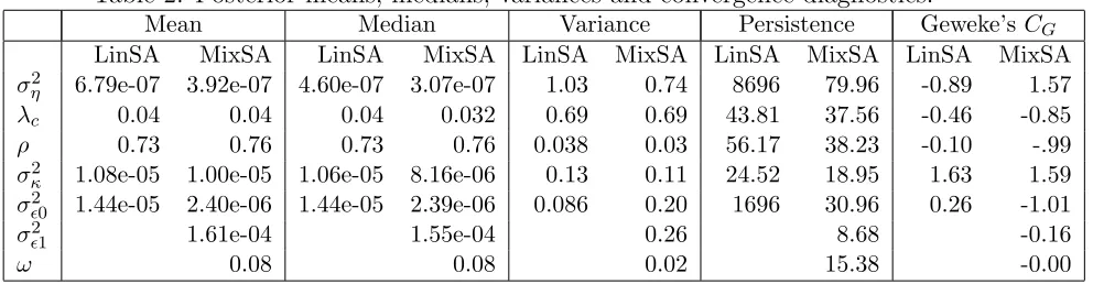
Our assessment of the convergence of the chain is based on the statistical properties of the observed chain. Table 2 summarizes some aspects of the posterior distribution of the parameters and presents the main convergence diagnostics. The acronim LinSA refers to the linear Gaussian model; MixSA to the mixture model for the SA series. If we let

VL=c0+ 2

l

X

j=1

wjcj, wj =

l−j l+ 1

denote the long run variance of a parameter sample path, wherecjis the autocovariance

at lagj and l is the truncation parameter,persistence is defined as SLdivided by the

variance (c0) (i.e., an estimate of the normalized spectral density at the zero frequency).

Moreover, if ψ(j) _{denotes the j-th sample of the GS scheme, after the burn-in period,}

and ¯ψadenotes the average of the firstnadraws, ¯ψb is the average of the lastnb draws

at the end of the convergence period, which are sufficiently remote to prevent any overlap, the Geweke’s convergence statistic (Geweke, 1992, 2005) is

CG=

¯

ψa−ψ¯b

p

VL,a/na+VL,b/nb

.

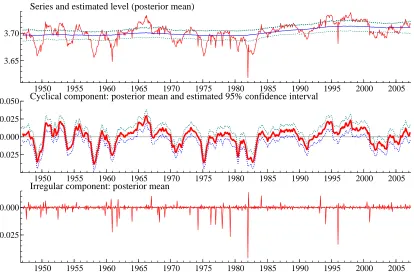
Figure 2 summarises aspects of the posterior distribution of the level, the cycle and the irregular for the linear Gaussian model. The posterior distribution of variance of the trend disturbances, σ2_η, and the weakly evolutive pattern of the estimated level confirm that unit root and stationarity tests may provide little guidance regarding the as to whether AWH are level stationary or difference stationary.

The plot reveals the presence of a number of observations which are highly influ-ential for the estimates of the cycle and the irregular. On the contrary, the estimated level is quite robust to the influence of those observations.

Modeling the irregular as a mixture of two Gaussian distributions has several ben-efits. First and foremost, the cycle estimates, plotted in figure 3, are smoother and are not affected by the outliers. The comparison of figure 3 with the estimated components for the standard linear model (see 2) suggests that part of the variability affecting the cycle estimates has been reallocated to the irregular component. This enables a clearer description of the business cycle phases and improves the characterisation of the turn-ing points. Secondly, the reliability of the cycle estimates increases, as the posterior variance of the cycle estimate reduces. That the mixture model outperforms the Gaus-sian linear model is confirmed by the comparison of the estimated marginal likelihoods under the two models. The following table reports the Chib and Jeliazkov (2001) es-timator of the marginal likelihood for the mixture modelM1 and the Gaussian model

Model logp(y|Ψ,Mk) logp(Ψk,Mk) log ¯p(Ψk|y,Mk) logm(y|Mk)

M1 1.77 9.45 19.42 -8.20

M2 137.50 8.19 21.36 124.44

Table 2: Posterior means, medians, variances and convergence diagnostics.

Mean Median Variance Persistence Geweke’s CG

LinSA MixSA LinSA MixSA LinSA MixSA LinSA MixSA LinSA MixSA

σ_η2 6.79e-07 3.92e-07 4.60e-07 3.07e-07 1.03 0.74 8696 79.96 -0.89 1.57

λc 0.04 0.04 0.04 0.032 0.69 0.69 43.81 37.56 -0.46 -0.85

ρ 0.73 0.76 0.73 0.76 0.038 0.03 56.17 38.23 -0.10 -.99

σ2

κ 1.08e-05 1.00e-05 1.06e-05 8.16e-06 0.13 0.11 24.52 18.95 1.63 1.59

σ_ǫ2₀ 1.44e-05 2.40e-06 1.44e-05 2.39e-06 0.086 0.20 1696 30.96 0.26 -1.01

σ_ǫ2₁ 1.61e-04 1.55e-04 0.26 8.68 -0.16

ω 0.08 0.08 0.02 15.38 -0.00

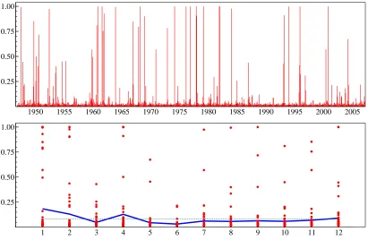
An interesting stylized fact emerges from the consideration of the estimated poste-rior probabilities of being in a high volatility state,P(St= 1|y,Ψ), which are displayed

in figure 6. The Monte Carlo estimate of the posterior mean ofωis 0.08, i.e. about one in ten observations is likely to be outlying. However, a closer inspection reveals that the the outlying observations are clustered in certain months of the year. This is clear from the bottom panel, which is the plot by month of the posterior probabilities. The solid line connects the monthly averages, and the dotted line is drawn at the average 0.08. In particular, the outliers are clustered in the initial months of the year, namely January (for which the average value of the posterior probability is 0.18), February, April and December. The average probability is a mere 0.03 in June.

If the estimated ˆpt = P(St = 1|y, ψ) are regressed on a constant and 11 seasonal

dummies, the test for the joint significance of the seasonal dummies takes the value 37.7 with a p-value of 8.9E-005. If the covariance matrix of the ordinary least squares estimator is corrected for heteroscedasticity and autocorrelation (see Newey and West, 1987), the evidence is unchanged. This suggests that the outlying observations have a marked periodic pattern.

6

Modeling Seasonality

The analysis of the seasonally adjusted data allows us to conclude that the Gaussian mixture model provides a useful representation of the data, allowing for the robust estimation of the cyclical component. Another important piece of evidence is that the outlying observations are not allocated randomly throughout the sample, but have a distinctive seasonal pattern. This may be the consequence of seasonal under and/or overadjustment. In this section we further investigate whether this is indeed the case, by estimating the same mixture model on the unadjusted series,yt, t= 1, . . . , n.

The model for the seasonal time series is specified as follows:

yt=ytSA+γt+β1Et+β2Lt, (18)

whereySA

t was given above in 1. The seasonal component,γt, is modeled as follows:

γt=z′tχt, χt=χt−1+ζt (19)

where z′

t = [D1t, . . . , Dst], with Djt = 1 in season j and 0 otherwise. The vector χt

contains the effects associated to each season and changes over time according to a multivariate random walk; ζt is a zero-mean multivariate white noise with covariance

matrix which enforces the constrainti′

sVar(ζt) = 0. This formulation is known in the

literature as the Harrison and Stevens (1976) specification. The distinguishing feature of this approach is that it is formulated directly in terms of the effect of a particular season, thereby enhancing flexibility needed to model seasonal heteroscedasticity (that is when there are seasons which are ‘more variables’ than others, see Proietti, 1998). The appropriate action for this model to deal with heteroscedasticity is to define the covariance matrix of the seasonal innovations as follows:

Var(ζt) = Ω =D−

1

i′ sDis

Disi′sD (20)

whereDis a diagonal matrix,D= diag{dj, j= 1, . . . ,12}. Our preferred specification

has the dj constant across groups of seasons. In particular, it envisages two groups

of seasons, made up respectively by January, February and April, and the remaining months, characterized by the two parameters,daanddb, which are constant across the

months belonging to the same group.

The regression component, β1Et+β2Lt, captures calendar effects: Et and Lt are

deterministic dummy variables taking value 1 if respectively Easter and Labor day fall within the observations week (that containing the 12th of each month).

6.1

Bayesian Estimation

Estimation is carried out in the same fashion as for the nonseasonal model in section (3). The unobserved states collected in the vector x now include also the seasonal component, i.e., x = {µt, ψt, γt, t= 0, . . . , n}. The vector of unknown parameters

Ψ = (σ2

η, σκ2, σǫ20, σ2ǫ1, λc, ρ, ω, β1, β2, da, db), is also updated to keep into account the

block of exogenous regressorsβ and the block of seasonal parametersd, introduced in the previous section.

To make Bayesian inference on this seasonal model we need to specify the prior distri-butions on these new parameters. To the extent of being noninformative, we specify the prior distribution for theβ’s as the Jeffrey’s reference prior for location parameters

p(β1, β2) ∝ 1, and we specify a Uniform distribution over a reasonable support for

both the seasonal parametersp(da, db)∝U(0,10]×U(0,10].

(v) Simulate β(i+1) ₌³_β(i+1) 1 , β

(i+1) 2

´

from the complete full conditional distribution

p³β|Λ(i+1),Σ(i+1), ω(i), x, S(i+1), y´∝N2 ¡

β|δ, τ2¢.

The posterior location and scale parameters are, respectively

τ−2 ₌¡_F′_F¢_{, δ =}¡_F′_F¢−1_F′_y˜

where F is a (n×2)−matrix of observations of the two regressors E1 and L1,

and y˜t=yt−ψt−µt−γt represent the difference between the original series yt

and the unobserved components µt, ψt and γt.

(vi) Simulate (da, db)(i+1) from the complete full conditional distribution

p³da, db|β(i+1),Λ(i+1),Σ(i+1), ω(i), x, S(i+1), y

´

∝ 1 |Ω|exp

( −1 2 n X t=1 ζ′ tΩ−1ζt

)

where ζt, t= 1,2, . . . , nandΩhave been defined in equation (19) and (20)

respec-tively.

The form of the full conditional distribution of the seasonal parameters (da, db) is not

known due to the way the two parameters enters the likelihood, through the relation specified in equation (20). To simulate from such a distribution we use a Gaussian multiplicative random walk Metropolis-Hastings algorithm where proposed values are generated using the relation

·

log ˜da

log ˜db

¸

=

"

logd(ai−1)

logd(_bi−1)

# + · ξa ξb ¸ , (21)

where³d(ai−1), d(_bi−1)

´

are the values sampled at the previous iteration of the algorithm,

while ³d˜a,d˜b

´

are the proposed values, and the two innovations terms (ζa, ζb) are

distributed accordingly to

· ξa ξb ¸ ∼N µ· 0 0 ¸ , · ν2 a 0

0 ν_b2

¸¶

.

The two variance parameters ¡ν2

a, νb2

¢

are calibrated in order to obtain a acceptance ratio equal to about 50−60%. The acceptance probability of this Metropolis step is equal to

α³d, d˜ (i−1)´_{= min} (

1, |Ωe| |Ω|exp

" −1 2 n X t=1 ζ′

tΩe−1ζt+

1 2 n X t=1 ζ′ t ³

Ω(i−1)´−1_ζ

t

#

J

)

whereΩ = Ωe ³d˜a,d˜b

´

, represent the proposed value of the variance ofζtand Ω(i−1) =

Ω³d˜a(i−1),d˜(_bi−1)

´

represents the previous value of the same quantity, while J =

¯ ¯ ¯ ¯d(di˜−a1)

a

˜

db

d(i−1)

b

¯ ¯ ¯ ¯,

6.2

Estimation Results

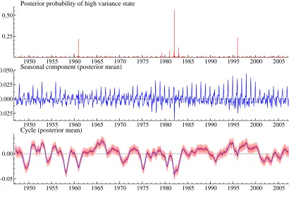
The estimation results presented in this section are based on a sample of 50000 draws from the Gibbs sampling scheme above, with a burn-in of 50000 iterations. The draws and the nonparametric estimates of the posterior densities are reproduced in figure 5. Table 3 reports the posterior means, medians, variances and convergence diagnostics of the parameters in the vector Ψ. It is remarkable that the estimated proportion of outlying observation is much reduced (the posterior mean of the mixture parameterω

is a mere 0.01). Actually, as it is shown in the first panel of figure 6, which displays the posterior probabilities of the high variance component, P(St = 1|y,Ψ), there is

one single observation belonging to the high volatility state with posterior probability greater than 0.5. Morever, the periodic feature has disappeared.

The second panel of the figure, which plots the estimated seasonal component, E(γt|y), reveals that the seasonal pattern is highly evolutive over time. Moreover, the

seasonal component absorbs a relevant part of the volatility that the model fitted to the SA series ascribed to the irregular component.

The cycle estimated from the model (bottom panel of figure 6) does not differ from that of the estimated using the MixSA model.

Table 3: Posterior means, medians, variances and convergence diagnostics.

Mean Median Variance Persistence Geweke’sCG

σ2

η 4.67e-007 3.38e-007 0.84 83.07 2.86

λc 0.047 0.041 0.10 23.42 0.87

ρ 0.74 0.74 0.03 28.01 -2.04

σκ2 1.03e-005 1.0e-05 0.10 38.05 -1.49

σ_ǫ2₀ 5.1e-07 4.8e-07 0.30 43.12 1.41

σ2

ǫ1 6637e-07 4886e-07 1.00 3.95 -0.23

ω 0.01 0.01 0.70 24.25 0.70

da 6.8e-06 6.8e-06 0.08 71.13 -1.89

db 1.1e-05 1.1e-05 0.08 82.49 -1.48

β1 0.01 0.01 0.08 11.17 -2.53

β2 0.01 0.01 0.13 1.30 -0.57

7

Conclusions

A

Model Selection

In this appendix we discuss in detail how we implement the Chib and Jeliazkov (2001) estimator of the marginal likelihood for the Gaussian mixture model defined in section 1. We evaluate each of the components of the posterior distribution of the parameters in equation 17 by means of the following steps.

(i) The draws from the full MCMC run described in section 3.3, are used to estimate the marginal density ordinate of the block parameters Σ, by

p(Σ∗_{|y) =} Z Y J

IG¡σ_J2|αJ, βJ

¢

p(ω,Λ, x, S|y) dω dΛdx dS

≃ 1 M

M

X

m=1 Y

J

IG³σ2_J|α(_Jm), β_J(m)´, J ={ǫ0, ǫ1, η, κ}

where nα(_Jm), β_J(m)oM

m=1,∀J are the parameters of the complete full conditional

distributions of the MCMC sampler described in section 3.3 point(iv), computed at the generated values.

(ii) Next, we fix the parameter Σ to Σ∗_{, and we obtain new draws}©_ω(g)_,Λ(g)_{, x}(g)_{, S}(g)ªG

g=1,

from a reduced MCMC with densities

p(ω|y, x,Λ,Σ∗_{, S), p(Λ|y, x,Σ}∗_{, ω, S), p(x|y, ω,Σ}∗_{,Λ, S), p(S|y, x, ω,Σ}∗_,Λ)

which are used to estimate the reduced posterior ordinate of the parameter ω

p(ω∗_|Σ∗_{, y) =}

Z

Be(ω|g0+nǫ0, h0+nǫ1)p(Λ, x, S|y,Σ∗) dΛdx dx

≃ 1 M

M

X

m=1

Be³ω|g0+n0(g), h0+n(1g) ´

,

where n(ǫg0) and n (g)

ǫ1 , are the number of observations allocated to the two

compo-nents of the mixture by the new reduced MCMC.

(iii) Finally, the full conditional density ordinate

p(Λ∗_|Σ∗_{, ω}∗_{, y) =}

Z

p(Λ∗_{|y, x,Σ}∗_{, ω}∗_{, S)p(x, S|y,Σ}∗_{, ω}∗_{) dx dS}

can not be estimated by Rao-Blackwellization, as in the previous cases, because the normalizing constant of the full conditional distribution p(Λ∗_{|y, x,Σ}∗_{, ω}∗_{, S)}

can be expressed as the ratio of two expectations and estimated by MC aver-ages of the MCMC output, in a similar way as we did in the previous steps. In what follows, we adapt the general formula of Chib and Jeliazkov (2001) to our problem of evaluating the normalizing constant of the reduced conditional ordinate p(ρ∗_{, λ}∗

c|Σ∗, ω∗, y). Let α(ρ, ρ∗|y, λc, ω∗,Σ∗, S) denotes the acceptance

probability of the M-H algorithm implemented within the Gibbs sampling to sample from the full conditional distribution of ρ, (see equation 10)1_{, and let}

q(ρ, ρ∗_{) the proposal distribution for the transition formρ to the new valueρ}∗2_,

then p(ρ∗_{, λ}∗

c|Σ∗, ω∗, y) can be expressed as the ratio of two expectations, in the

following way

p(ρ∗_|Σ∗_{, ω}∗_{, y) =} E1[α(ρ, ρ∗|y, λc, ω∗,Σ∗, S)q(ρ, ρ∗)]

E2[α(ρ∗, ρ|y, λc, ω∗,Σ∗, S)]

, (22)

where the expectation at the numerator E1 is taken with respect to the density

p(ρ, λc, x, S|y, ω∗,Σ∗), while the expectation at the denominatorE2is taken with

respect to the densityp(λc, x, S|y, ρ∗,Σ∗, ω∗)q(ρ∗, ρ|y, λc,Σ∗, ω∗, S). Each of the

integrals in equation 22 can be estimated by the output of the MCMC algorithm.

1. To estimate the numerator, fix Σ andωto the maximum a posteriori (Σ∗_{, ω}∗_),

run a reduced MCMC with densities

p(Λ|y, x,Σ∗_{, ω}∗_{, S), p(x|y, ω}∗_,Σ∗_{,Λ, S), p(S|y, x, ω}∗_,Σ∗_,Λ),

and take the draws©Λ(l)_{, x}(l)_{, S}(l)ªL

l=1to average the quantityα(ρ, ρ∗|y, λc, ω∗,Σ∗, S)q(ρ, ρ∗),

i.e.

b

E1[α(ρ, ρ∗|y, λc, ω∗,Σ∗, S)q(ρ, ρ∗)]

≃ 1 L

L

X

l=1

α³ρ∗_{, ρ|y, λ}(l)

c , ω∗,Σ∗, S(l)

´

q³ρ(l), ρ∗´_.

2. For the denominator of equation 22, because the expectation is conditioned on ρ∗_{, we run an additional reduced MCMC algorithm with ρ fixed at ρ}∗_,

and full conditionals

p(λc|y, x,Σ∗, ω∗, ρ∗, S), p(x|y, ω∗,Σ∗, λc, ρ∗, S), p(S|y, x, ω∗,Σ∗, ρ∗, λc).

At each iteration of this reduced sampler, a value ofρis drawn from the pro-posal distribution of the Metropolis stepq(ρ∗_{, ρ), conditional on the previous}

draws of ³λ(ch), x(h), S(h)

´

from the reduced sampler, i.e.

ρ(h)∼q(ρ∗_{, ρ)}

1_{The acceptance probability of the M-H step, α(ρ, ρ}∗_{|y, λ}

c, ω∗,Σ∗, S), depends on the parameters

(λc, ω,Σ) and on the latent vectorS, through the likelihood ratio.

2_{The proposal distribution is a Beta distribution with mean equal to the previous value of the sub-chain,}

leading to the samplenλ(ch), x(h), S(h), ρ(h)

oH

h=1 from the distribution

p(λc, x, S|y, ρ∗,Σ∗, ω∗)q(ρ∗, ρ).

The denominator of equation 22 is then estimated by

b

E2[α(ρ∗, ρ|y, λc, ω∗,Σ∗, S)] =

1

H

H

X

h=1

α³ρ∗_{, ρ}(h)_{|y, λ}(h)

c , ω∗,Σ∗, S(h)

´

,

and this allows us to estimate the ordinate p(ρ∗_|y,Σ∗_{, ω}∗₎

b

p(ρ∗_|y,Σ∗_{, ω}∗_{) =} Eb1[α(ρ, ρ∗|y, λc, ω∗,Σ∗, S)q(ρ, ρ∗)]

b

E2[α(ρ∗, ρ|y, λc, ω∗,Σ∗, S)]

(23)

Exactly in the same way as we did for the parameterρ, we can now estimate the ordinate for λc, using the following relation

b

p(λ∗

c|Σ∗, ω∗, ρ∗, y) =

b

E1[α(λc, λ∗c|y, ρ∗, ω∗,Σ∗, S)q(λc, λ∗c)]

b

E2[α(λ∗c, λc|y, ρ∗, ω∗,Σ∗, S)]

, (24)

where the expectation in the numerator of equation 24 is taken with respect to

p(λc, x, S|y, ρ∗,Σ∗, ω∗) and it is estimated by averagingα(λc, λc∗|y, ρ∗, ω∗,Σ∗, S)q(λc, λ∗c)

using the same draws form the reduced MCMC described in the previous point 2. The expectation in the denominator of equation 24 is taken with respect to the distributionp(x, S|y, ρ∗_,Σ∗_{, ω}∗_{, λ}∗

c)q(λ∗c, λc), and it is estimated by averaging

α(λ∗

c, λc|y, ρ∗, ω∗,Σ∗, S) using the output of a reduced MCMC with densities

p(x|y, ω∗_,Σ∗_{, λ}∗

c, ρ∗, S), p(S|y, x, ω∗,Σ∗, λ∗c, ρ∗)

with the additional simulation, at each step, of a random variates from the pro-posal distribution q(λ∗

References

Bernardo, J. M. (2005). Reference Analysis. InHandbook of Statistics, 25, Elsevier, North-Holland, Amsterdam, 459-507.

Casella, G., and Robert, C. P. (2004). Monte Carlo Statistical Methods. Springer Texts in Statistics. Springer, New York.

Chen M.-H and Q.-M. Shao (1997). On Monte Carlo methods for estimating ratios of normalizing constants. The Annals of Statistics, 25, 1563-1594.

Chib, S. (1995). Marginal likelihood from the Gibbs output. Journal of the Amer-ican Statistical Association, 90, 1313-1321.

Chib, S., and Jeliazkov (2001). Marginal likelihood from the Metropolis-Hastings output. Journal of the American Statistical Association, 96, 270-281.

Chipman, H., E. I. George, and E. McCulloch (2001). The practical implementation of Bayesian model selection. IMS Lecture Notes - Monograph series (2001), 38.

Cho, J-O. and Cooley, T. F. (1994). Employment and hours over the business cycle.

Journal of Economic Dynamics and Control, 18, 411-432.

Conference Board (2001). Business Cycle Indicators Handbook. Available at

http://www.conference-board.org/pdf free/economics/bci/BCI-Handbook.pdf

de Jong, P., and Shephard, N. (1996). The simulation smoother. Biometrika, 2, 339-50.

de Pooter, M. D., Segers, R., and van Dijk, H. K. (2006). On the Practice of Bayesian Inference in Basic Economic Time Series Models using Gibbs Sampling.

Tinbergen Institute Discussion Paper, 076/4.

Diebold, J. and Robert, C. P., (1994). Estimation of finite mixture distributions through Bayesian sampling. Biometrika, 56, 363 - 375.

Doornik, J.A. (2006),Ox: An Object-Oriented Matrix Programming Language, Tim-berlake Consultants Press, London.

Durbin, J., and S.J. Koopman (1997). Monte Carlo maximum likelihood estimation of non-Gaussian state space model. Biometrika, 84, 669-84.

Durbin, J., and S.J. Koopman (2001). Time Series Analysis by State Space Methods. Oxford University Press, Oxford.

Fr¨uhwirth-Schnatter, S. (2006). Finite Mixture and Markov Switching Models. Springer Series in Statistics. Springer, New York.

Gal´ı, J., and Rabanal, P. (2005). Technology Shocks and Aggregate Fluctuations: How Well Does the RBC Model Fit Postwar U.S. Data? In NBER Macroeco-nomics Annual 2004, (Mark Gertler and Kenneth Rogoff eds.), 22588. Cam-bridge, MIT Press.

Gelman, A., and X.-L. Meng (1998). Simulating normalizing constants: from im-portance sampling to bridge sampling to path sampling Statistical Sciences, 18, 163-185.

Geman, S. and Geman, D. (1984). Stochastic Relaxation, Gibbs distributions and the Bayesian restoration of images. IEEE Transactions on Pattern Analysis and Machine Intelligence, 6, 721-741.

Geweke, J., (1992). Evaluating the Accuracy of Sampling-Based Approaches to the Calculation of Posterior Moments. In J. M. Bernardo, J. Berger, A. P. Dawid, and A. F. M. Smith, eds., Bayesian Statistics 4, Oxford University Press, pp. 169-193.

Geweke, J., (2005). Contemporary Bayesian Econometrics and Statistics. Wiley Series in Probability and Statistics. Wiley, Hoboken.

Giordani, P., Kohn, R., and van Dijk, D. (2007). A unified approach to nonlinearity, structural change, and outliers. Journal of Econometrics, 127, 112–133.

Glosser, S. M., and Golden, L. (1997). Average work hours as a leading economic variable in US manufacturing industries. International Journal of Forecasting, 13, 175–195.

Harrison, P. and C. Stevens (1976). Bayesian forecasting. Journal of the Royal Statistical Society. Series B, 38, 205-247.

Harvey, A.C. (1989). Forecasting, Structural Time Series and the Kalman Filter, Cambridge University Press, Cambridge, UK.

Harvey, A. C., Trimbur, T. M., and Van Dijk, H. K. (2007). Trends and cycles in economic time series: A Bayesian approach. Journal of Econometrics, 140, 618 - 649.

Hastings W. K., (1970). Monte Carlo sampling methods using Markov chains and their applications. Biometrika, 57, 97-109.

Kass, R. E., and A. E. Raftery. (1995). Bayes factors. Journal of the American Statistical Association, 90, 773-795.

Koopman S.J., Shepard, N., and Doornik, J.A.: “Statistical algorithms for models in state space using SsfPack 2.2”,Econometrics Journal, 2 (1999), 113-166.

Newey, W.K., and West, K.D. (1987). A Simple, Positive Semi-Definite, Het-eroskedasticity and Autocorrelation Consistent Covariance Matrix. Economet-rica, 55, 703–708.

Meng, X.-L, and S. Schilling (2002). Warp bridge sampling. Journal of Computa-tional and Graphical Statistics, 11, 552-586.

Metropolis, N., A. W. Rosenbluth, M. N. Rosenbluth, A. H. Teller, E. Teller, (1953). Equations of state calculations by fast computing machines. Journal of Chemical Physics, 21, 1087-1091.

Figure 1: Average weekly hours in manufacturing: seasonally adjusted series (logarithms) and unadjusted series. The shaded areas flag recessionary periods, according to the NBER chronology.

1950 1955 1960 1965 1970 1975 1980 1985 1990 1995 2000 2005

3.625 3.650 3.675 3.700 3.725

3.750 Seasonally adjsted series

1950 1955 1960 1965 1970 1975 1980 1985 1990 1995 2000 2005

3.65 3.70 3.75

Figure 2: Seasonally adjusted AWH, linear Gaussian model: estimates of unobserved com-ponents.

1950 1955 1960 1965 1970 1975 1980 1985 1990 1995 2000 2005

3.65 3.70

Series and estimated level (posterior mean)

1950 1955 1960 1965 1970 1975 1980 1985 1990 1995 2000 2005

−0.025 0.025

Cyclical component: posterior mean and estimated 95% confidence interval

1950 1955 1960 1965 1970 1975 1980 1985 1990 1995 2000 2005

−0.02 0.00

Figure 3: Seasonally adjusted AWH, model with normal mixture irregular: estimates of unobserved components.

1950 1955 1960 1965 1970 1975 1980 1985 1990 1995 2000 2005

3.65 3.70

Series and estimated level (posterior mean)

1950 1955 1960 1965 1970 1975 1980 1985 1990 1995 2000 2005

−0.025 0.000 0.025

0.050 Cyclical component: posterior mean and estimated 95% confidence interval

1950 1955 1960 1965 1970 1975 1980 1985 1990 1995 2000 2005

−0.025 0.000

Figure 4: Seasonally adjusted AWH, model with normal mixture irregular: posterior prob-abilities of high variance component, P(St= 1|y,Ψ) (top panel), and monthplot.

1950 1955 1960 1965 1970 1975 1980 1985 1990 1995 2000 2005

0.25 0.50 0.75 1.00

1 2 3 4 5 6 7 8 9 10 11 12

Figure 5: Unadjusted AWH series model: MCMC draws and posterior densities of the parameters.

//

0 12500 25000 37500 50000 1e−6

2e−6 3e−6

4e−6 GS draws ση

2

0 2e−6 4e−6

Density σ_η2

0 12500 25000 37500 50000 1.0e−5

1.5e−5

GS draws σ_κ2

1.0e−5 1.5e−5 Density σ_κ2

Sigma Cycle

−2 0 2

0

1 GS draws AR pars. (φ1,φ2)

0.0 0.1 0.2

Density λ_c

0 12500 25000 37500 50000 5e−7

1e−6 1.5e−6

GS draws σ_ε02

5e−7 1e−6 1.5e−6 Density σ_ε02

0 12500 25000 37500 50000 0.01

0.02 GS draws σε1

2

0.00 0.01 0.02 Density σ_ε12

0 12500 25000 37500 50000 0.950

0.975

1.000 GS draws ω

0.950 0.975 1.000 Density ω

0 12500 25000 37500 50000 7.5e−6

1.0e−5 1.25e−5

1.5e−5 Seasonal variances_d a db

7.50e−6 1.25e−5 Density

Density seas. var. Density

Density seas. var. Density

Density seas. var. da db

0 12500 25000 37500 50000 0.005

0.010 0.015

Regression parameters β2 β1

0.005 0.010 0.015 Density

Density Density Density Density Density regr. par

Figure 6: Estimated cycle (posterior mean of ψt) and seasonal component (posterior mean

of γt): posterior probabilities of high variance component, P(St = 1|y,Ψ) (top panel), and

monthplot.

1950 1955 1960 1965 1970 1975 1980 1985 1990 1995 2000 2005

0.25 0.50

Posterior probability of high variance state

1950 1955 1960 1965 1970 1975 1980 1985 1990 1995 2000 2005

−0.025 0.000 0.025

0.050 Seasonal component (posterior mean)

1950 1955 1960 1965 1970 1975 1980 1985 1990 1995 2000 2005

−0.05 0.00