http://dx.doi.org/10.4236/ijcns.2014.71007
Compression of ECG Signals Based on DWT and
Exploiting the Correlation between ECG Signal Samples
Mohammed M. Abo-Zahhad, Tarik K. Abdel-Hamid, Abdelfatah M. Mohamed Electrical and Electronics Engineering Department, Faculty of Engineering, Assiut University, Assiut, Egypt
Email: [email protected]
Received December 11, 2013; revised January 3, 2014; accepted January 9, 2014
Copyright © 2014 Mohammed M. Abo-Zahhad et al. This is an open access article distributed under the Creative Commons Attribu-tion License, which permits unrestricted use, distribuAttribu-tion, and reproducAttribu-tion in any medium, provided the original work is properly cited. In accordance of the Creative Commons Attribution License all Copyrights © 2014 are reserved for SCIRP and the owner of the intellectual property Mohammed M. Abo-Zahhad et al. All Copyright © 2014 are guarded by law and by SCIRP as a guardian.
ABSTRACT
This paper presents a hybrid technique for the compression of ECG signals based on DWT and exploiting the correlation between signal samples. It incorporates Discrete Wavelet Transform (DWT), Differential Pulse Code Modulation (DPCM), and run-length coding techniques for the compression of different parts of the signal; where lossless compression is adopted in clinically relevant parts and lossy compression is used in those parts that are not clinically relevant. The proposed compression algorithm begins by segmenting the ECG signal into its main components (P-waves, QRS-complexes, T-waves, U-waves and the isoelectric waves). The resulting waves are grouped into Region of Interest (RoI) and Non Region of Interest (NonRoI) parts. Consequently, loss- less and lossy compression schemes are applied to the RoI and NonRoI parts respectively. Ideally we would like to compress the signal losslessly, but in many applications this is not an option. Thus, given a fixed bit budget, it makes sense to spend more bits to represent those parts of the signal that belong to a specific RoI and, thus, re- construct them with higher fidelity, while allowing other parts to suffer larger distortion. For this purpose, the correlation between the successive samples of the RoI part is utilized by adopting DPCM approach. However the NonRoI part is compressed using DWT, thresholding and coding techniques. The wavelet transformation is used for concentrating the signal energy into a small number of transform coefficients. Compression is then achieved by selecting a subset of the most relevant coefficients which afterwards are efficiently coded. Illustrative exam- ples are given to demonstrate thresholding based on energy packing efficiency strategy, coding of DWT coeffi- cients and data packetizing. The performance of the proposed algorithm is tested in terms of the compression ratio and the PRD distortion metrics for the compression of 10 seconds of data extracted from records 100 and 117 of MIT-BIH database. The obtained results revealed that the proposed technique possesses higher compres- sion ratios and lower PRD compared to the other wavelet transformation techniques. The principal advantages of the proposed approach are: 1) the deployment of different compression schemes to compress different ECG parts to reduce the correlation between consecutive signal samples; and 2) getting high compression ratios with acceptable reconstruction signal quality compared to the recently published results.
KEYWORDS
ECG Signal Segmentation; Lossless and Lossy Compression Techniques; Discrete Wavelet Transform; Energy Packing Efficiency; Run-Length Coding
1. Introduction
In technical literatures, numerous ECG compression al- gorithms have been developed in the last thirty years. They may be defined either as reversible methods (offer- ing low compression ratios but guaranteeing an exact or near-lossless signal reconstruction), irreversible methods
most suitable. However, if compressed data has to be stored on low-capacity data supports, an irreversible compression would be necessary. The scalable tech-niques clearly suit data transmission. ECG compression techniques can be categorized into: direct time-domain techniques; transformed frequency-domain techniques and parameters optimization techniques.
1) Direct Signal Compression Techniques: Direct me- thods involve the compression performed directly on the ECG signal. Many of the time domain techniques for ECG signal compression are based on the idea of ex- tracting a subset of significant signal samples to repre- sent the original signal. The key to a successful algorithm is the development of a good rule for determining the most significant samples. Decoding is based on interpo- lating this subset of samples. The traditional ECG time domain compression algorithms all have in common that they are based on heuristics in the sample selection pro- cess. This generally makes them fast, but they all suffer from sub-optimality [1].
2) Transformed ECG Compression Methods: Trans- form domain methods, operate by transforming the ECG signal into another domain. These methods mainly utilize the spectral and energy distributions of the signal, and properly encoding the transformed output. Signal recon- struction is achieved by an inverse transformation pro- cess. This category includes traditional transform coding techniques applied to ECG signals such as the Karhunen- Loève transform [2], Fourier transform [3], Cosine trans- form [4], subband-techniques [5], vector quantization (VQ) [6], and more recently the wavelet transform (WT) [7]. The wavelet decomposition splits the signal into ap- proximation and detail coefficients, using finite impulse response digital filters. Wavelet-based ECG compression methods have been proved to perform well. The ability of DWT to separate out pertinent signal components has led to a number of wavelet-based techniques which su- persede those based on traditional Fourier methods.
3) Optimization Methods for ECG Compression: More recently, many interesting optimization based ECG com- pression methods, the third category, have been devel- oped. The goal of most of these methods is to minimize the reconstruction error given a bound on the number of samples to be extracted or the quality of the recon- structed signal to be achieved. In [8], the goal is to mi- nimize the reconstruction error given a bound on the number of samples to be extracted. This leads to the best possible representation in terms of the number of ex- tracted signal samples, but not necessarily in terms of bits used to encode such samples. In [9], the bit rate has been taken into consideration in the optimization process. The key issue is to choose the most suitable method for the ECG signals application. What is intended through this paper is to obtain the highest data reduction
by preserving the clinical characteristics of the signal.
2. Algorithm Description
The QRS complex of an ECG cycle occupies a relatively low percentage of the whole cycle, but it is the most im- portant portion from a diagnostic point of view for many diseases. If this portion suffers from high error and other ECG cycle portions do not have errors, artificially wrong diagnostic decisions may happen. Hence, a given distor- tion in one portion does not inevitably have the same influence as the same distortion in another portion. For these reasons the proposed compression algorithm fo- cuses on the provision of different compression ratios for different portions of the heart cycle, where the RoI is selected according to context information (disease/car- diac event to detect status of the patient).
Ideally we would like to compress the signal losslessly, but in many applications this is not an option. Thus, for a given fixed bit budget, it makes sense to spend more bits to represent those parts of the signal that belong to a spe- cific clinically relevant parts, while allowing other parts to suffer larger distortion. Consequently, the performance assessment of the proposed methodology should take this into account. In general, the main goal for any compres- sion procedure consists in reducing as much as possible the bit-rate of the signal by keeping an acceptable quality or, equivalently, by improving as much as possible the quality for a fixed assigned bit-rate. Thus, the two most important parameters are the compression ratio and the quality of the signal. The framework of the compression process is summarized in the following.
2.1. Patient Side
1) Capture the ECG signal from the patient or prepare an uncompressed signal from a database.
2) If the signal is captured from a patient, clean it from artifacts and remove the signal mean and normalize it. In case of picking the signal from a database, remove its mean and normalize the resulting mean-removed signal. In this paper, all signals considered are extracted from MIT-BIH database.
3) Segment the signal into RoI part (QRS-complex and possibly P- T- and U-waves) and the NonRoI part (the remaining parts representing the difference between the original ECG signal and the RoI part).
4) Compress the RoI part using DPCM lossless com- pression method and applying proper quantization.
5) Encode the resulting quantized residuals into binary stream by run-length coding algorithm.
6) Compress the NonRoI part using DWT lossy com- pression technique and applying proper thresholding and quantization.
into binary stream by run-length coding algorithm. 8) Packetize the data and prepare the data header.
2.2. Transmission Side
1) Guarantee network connection (Intranet or Internet) and/or wireless transmission facilities.
2) Transmit the data header, the binary stream of the RoI part and that of the NonRoI part consecutively.
2.3. Reception Side
1) Depacketize the received binary stream into the header, binary stream of the RoI and that of the NonRoI parts respectively.
2) Convert the binary streams of the header into the basic information important for ECG signal reconstruc- tion such as length of RoI stream, length of NonRoI stream, start and end of each wave in RoI and NonRoI parts.
3) Convert the binary streams of both RoI and NonRoI parts into their equivalent decimal numbers.
4) Apply inverse DPCM for RoI part and apply inverse wavelet transform for NonRoI part.
5) Decompose the resulting time-domain RoI and NonRoI parts into QRS-waves, T-waves, P-waves, U- waves and isoelectric-waves.
6) Use the obtained data in the above steps to recon- struct the ECG signal.
7) Calculate the compression ratio and the error meas- ures for evaluation and comparison.
8) Output the reconstructed ECG signal for medical investigation.
3. Features Extraction and Locating ECG
Signal Critical Points
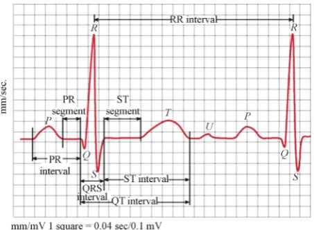
The significant features of the ECG signal, such as the R point, RR interval, and amplitude of R point, average RR interval, QRS duration and existence of QRS should be extracted for the next compression stage. The significant features are shown in Figure 1; where each heartbeat signal starts by the P wave and ends at the next P wave of the following heartbeat. Moreover, the heartbeat can be divided into a crucial part and a plain part [10].
[image:3.595.311.538.84.250.2]The QRS complex wave is the most important part of the cardiology system to determine arrhythmia. The P and T waves also have high level of information and the remaining plane parts contain less information. Therefore, in this work, the ECG signal is segmented into parts and the number of bits is assigned differently according to the importance of each part. For example, more bits are as- signed to the RoI part, and fewer bits are assigned to the NonRoI part. The critical points of the ECG signal are very important in defining its RoI and NonRoI parts. These critical points are namely; the P, Q, R, S, T and U
Figure 1. Significant features of one beat ECG signal.
points. In the following a robust algorithm for the detec- tion of the locations of these points using the properties of the real time analysis of the ECG signal is described.
The R-wave detection is the most important process in the segmentation algorithm because all coming processes are based on the locations of the R-peaks. This has been carried out by adaptive thresholding the ECG signal. The threshold levels used in this work are not constant for all ECG signal beats. This overcomes the error in detecting the R-wave as a result of the unexpected changes in the ECG signal from beat to beat. Each beat is defined by the R-R interval that has a length from about 0.14 sec up to 1.2 sec (corresponds to 144 samples to 432 samples). To carry out the R-peak detection process, a window of length greater than 432 samples should be used. The width of the widow must be selected carefully to avoid error detection of the R-wave of the ECG signal. In this study a window of width 500 samples is selected. Then the maximum value of the ECG signal within this win-dow is calculated.
The window is slide to the right by one sample and the maximum value within the new window is calculated. This process is repeated until the left edge of the window reaches the last sample of the signal. This process yields to the upper threshold levels of each beats. The lower threshold levels are calculated as a factor of the upper threshold levels. It has been found that a factor of half is suitable for detecting the R-peaks. The next step is the thresholding of the ECG signal with the resulted thshold levels and finding the maximum points of the re-sulting signal that represents the R peaks.
samples after the location of the R-peak has been carried out for detecting the Q- and S-peaks.
The T-, U- and P-peaks are located between the Q- and next S-peaks. Firstly, we define the SQ segment as the region from the location of the current S-peak up to the location of the following Q-peak. The of maximum and minimum points in the SQ segment are determined by adopting the same method used to find the R-peaks where the sliding window width used is selected to be equal to one-tenth the width of the SQ segment. The points of the maximum of the windows is picked and considered as the T-, U- and P-peaks after avoiding mul- tipoint problems. According to the morphology of the ECG signal and after the consultations with cardiologists, the detected peaks are considered as the peaks of the T-, U- and P-waves according to the following rules.
• If there are no peaks detected, then no T-, U- or P-peak exists.
• If there is only one peak detected, then this peak will be the T-peak and there is no U-peak or P-peak.
• If there are two peaks detected, the first peak will be the T-peak and the next peak will be the P-peak and there is no U-peak.
[image:4.595.59.288.536.706.2]• If there are three peaks or more detected the first peak will be the T-peak and the next peak will be the U- peak and the last peak will be the P-peak.
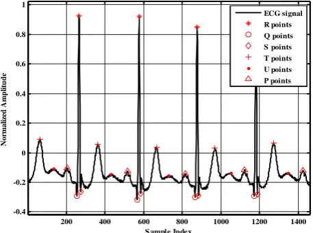
Figure 2illustrates the ECG signal with P, Q, R, S, T and U points indicated.
4. Segmentation of ECG Signal into Waves
The ECG segment is defined as the period between the end of a wave to the start of the next wave. After finding the P-, Q-, R-, S-, T- and U-peaks locations, the segments PQ, ST, TU, and UP are defined as the portions of the ECG signal between the two adjacent peak locations. In each of these segments, an isoelectric wave exists. If the
Figure 2. It illustrates the ECG signal with P, Q, R, S, T and U points indicated.
start and end locations of each isoelectric wave is deter- mined, the starts and ends locations of all other waves can be determined. The idea of finding the start and end locations of isoelectric waves is centered in finding the longest period with lowest standard deviation (STD) in each segment. This is carried out as follows:
• Locate the interval V between the two adjacent points defining the segment, (i.e. P and Q, S and T, T and P).
• Calculate the STD of the regions whose start is the first sample of the interval V and whose ends are points after the first point; e.g. Std(1) = STD(V(1:2), std(2) = STD(V(1:3)), std(3) = STD(V(1:4)), ... std(n) = STD(V(1:n + 1)).
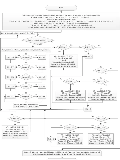
• Repeat the last step for the next sample of the interval V and so on until the last sample of the interval V. The decomposition of the ECG signal into its waves is illustrated in the flowchart shown in Figure 3. As a result, the start and end locations of the ECG waves are de- tected.
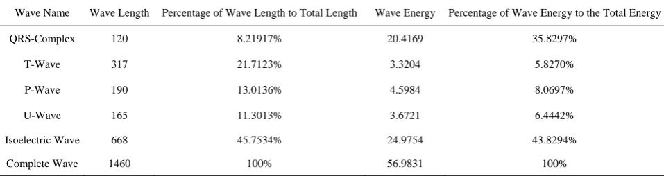
Pwave_st=Waves{1}; Pwave_ed=Waves{2}; QRSwave_st=Waves{3}; QRSwave_ed=Waves{4}; Twave_st = Waves{5}; Twave_ed= Waves{6}; Uwave_st= Waves{7}; Uwave_ed = Waves{8}; isoelectric_st = SEG{1}; and isoelectric_ed = SEG{2}; After finding the region that achieves lowest STD and longest length; the start and end of each isoelectric wave is determined. Consequently, the starts and ends of all other waves are determined. To illustrate the importance of the ECG signal’s components, the energy and the number of samples (wave length) of each component are calculated. Table 1 includes the calculated energies and wave lengths of different ECG components for 1460 samples from record 103. From this table it can be ob- served that the longest component is the isoelectric wave in which about 45% of the ECG signal energy and num- ber of samples are concentrated. Fortunately, these waves have no clinical importance. Thus, it will be considered as the main component of the Non-RoI part. In contrary to that the energy of the QRS-complexes is about 36% of the signal energy with smallest number of samples (about 8%). This part of the signal is very important from clini- cal point of view. So, it will be considered as the main component of the RoI part. The T- and P-waves contri- buted by 5.8% and 8.1% of the energy respectively; however the length of the T-waves is 1.7 times that of the P-waves. Thus, P-wave is a candidate for RoI part and T-wave is a candidate for NonRoI part. Considering ei- ther of them in RoI or NonRoI depends on the patient’s case and the patient’s heart disease [10]. Table 2 in- cludes the 74 start and end indices of all the ECG signal waves. Investigation of this table reveals that, among these 36 indices are for isoelectric-waves and there exists an isoelectric-wave between each two other waves. Since
200 400 600 800 1000 1200 1400
-0.4 -0.2 0 0.2 0.4 0.6 0.8 1
S ample Index
N or mal iz ed A mp li tu d e ECG signal R points Q points
Table 1. Energy distribution and wave lengths of ECG components for 1460 samples of record 103.
Wave Name Wave Length Percentage of Wave Length to Total Length Wave Energy Percentage of Wave Energy to the Total Energy
QRS-Complex 120 8.21917% 20.4169 35.8297%
T-Wave 317 21.7123% 3.3204 5.8270%
P-Wave 190 13.0136% 4.5984 8.0697%
U-Wave 165 11.3013% 3.6721 6.4442%
Isoelectric Wave 668 45.7534% 24.9754 43.8294%
Complete Wave 1460 100% 56.9831 100%
Table 2. The start and end indices of all ECG signal waves.
Beat Number
T-Wave Isoelectric-Wave U-Wave Isoelectric-Wave
Start End Start End Start End Start End
1 1 89 90 125 126 153 154 191
2 331 387 388 422 423 455 456 500
3 635 689 690 721 722 757 758 802
4 936 992 993 1034 1035 1069 1070 1107
5 1240 1299 1300 1336 1337 1369 1370 1410
Beat Number
P-Wave Isoelectric-Wave QRS-Wave Isoelectric-Wave
start end Start end start end start end
1 192 225 226 251 252 285 286 330
2 501 536 537 562 563 591 592 634
3 803 837 838 863 864 892 893 935
4 1108 1142 1143 1167 1168 1195 1196 1239
5 1411 1460
the start of each wave is less than the end of the preced- ing wave by one, the start of the next wave can be di- rectly determined. The only two exceptions are the start index of the first wave that is 1 and the end index of the last wave that is the signal length. Using these facts, the 74 entries of Table 2 can be obtained from only 36 en- tries.
From the above discussion, it can be deduced that only the 36 entries need to be included in HeaderW and no need to transmit the start and end of isoelectric waves. It should be noticed that the starts and ends of isoelectric waves are generated in the receiver side using the fol- lowing Matlab code.
n = length (HeaderW); SortedHW = sort (HeaderW); k = 0;
for i = 2 : 2 : n − 1 k = k + 1; startiso (k) = SortedHW (i) + 1; endiso(k) = SortedHW (i + 1) − 1; end
Running the above code results the following starts and ends of the isoelectric waves.
startiso = [90 154 226 286 388 456 537 592 690 758 838 893 993 1070 1143 1196 1300 1370]
endiso = [125 191 251 330 422 500 562 634 721 802 863 935 1034 1107 1167 1239 1336 1410]
These indices will be deployed in the reconstruction of the signal in the receiver side. To finalize this section, the preparation for ECG signal segmentation into RoI and NonRoI parts is summarized in the following:
1) The ECG signal is decomposed into its waves and these waves are stored in the vectors: Twaves, Uwaves, Pwaves, and QRSwaves. These waves will be grouped into RoI and NonRoI parts.
[image:6.595.59.539.256.497.2]3) The starts and ends of all sub-waves are defined and stored in HeaderW, e.g. the first QRS sub-wave starts at EQwave1 and ends at EQwave1. Each value is repre- sented by 11-bits. The 11-bits can accommodate a signal of length 2048. For longer ECG signals, this number should be increased.
4) The starts and ends of the isoelectric waves are de- duced from HeaderW using the Matlab code described above.
5. Compression of ECG Signal Based on
Segmentation into RoI and NonRoI Parts
5.1. Signal Segmentation into RoI and NonRoI Parts
In the previous section segmentation of ECG signal into its waves has been discussed. For the purpose of signal compression, the following three cases of constructing the RoI and NonRoI parts from these waves are:
1) QRS-waves are considered in RoI and the remain- ing waves are in NonRoI.
[
]
[
]
RoI QRSwave and
NonRoI TwaveUwavePwaveisoelectricwave
=
= (1)
2) QRS- and T-waves are considered in RoI and the remaining waves are in NonRoI.
[
]
[
]
RoI QRSwaveTwave and
NonRoI UwavePwaveisoelectricwave
=
= (2)
3) QRS-, T- and P-waves are considered in RoI and the remaining waves are in NonRoI.
[
]
[
]
RoI QRSwaveTwavePwave and
NonRoI Uwaveisoelectricwave
=
= (3)
Since the RoI is the most important part of the signal for medical diagnostic purposes, it must be coded with a lossless compression algorithm. The NonRoI part of the ECG signal has not had a considerable effect of medical diagnostic. For this reason, this part is compressed by using lossy compression technique. For this purpose DP- CM technique is used for compressing the ROI part of the signal. However, the NonRoI part of the signal is compressed using wavelet based compression technique. To send the information related to the compression stage, the number of signal samples in the RoI (Len_RoI) and the number of signal samples in the NonRoI (Len_ NonRoI) should be added to Header1 and each is repre- sented by 11-bits. In the following subsections the algo- rithms developed for the compression of RoI part using DPCM and NonRoI part using DWT are presented. Al- though the discussion presented in the following subsec- tions is limited to the first case described by Equation (1), all algorithms that will be discussed can be adopted by
reconstructing RoI and NonRoI vectors according to Eq- uations (2) and (3). Figure 4 illustrates the ECG signal after its decomposition into RoI and NonRoI parts, where all P waves, QRS waves, T waves, U waves, and isoelec- tric waves are arranged in groups.
5.2. Compression of RoI Part Using Differential Pulse Code Modulation
Amongst the different direct data compression tech-niques, which are based on the detection of redundancies on the original signal, pulse code modulation (PCM) pro- vides simple and fast compression schemes. In PCM technique each sample of the waveform is encoded inde- pendently of any other sample. An encoding scheme that exploits the redundancy in the samples will result in higher compression ratio and a lower bit rate for the source output. A relatively simple solution is to encode the differences between successive signal samples rather than the samples themselves, rendering the differential pulse code modulation (DPCM) technique. The equation for calculating a DPCM sequence is
( ) ( ) (
1)
e n =x n −x n− (4)
where, e(n) is the prediction error. Since differences be- tween samples are expected to be smaller than the actual sampled amplitudes, fewer bits are required to represent the differences. A block diagram of a DPCM encoder and decoder used in this subsection is shown in Figure 5(a). A natural extension of the DPCM operation is to predict the value of the current sample based on the pre- vious m samples using Linear Prediction (LP) technique, as shown in Figure 5(b).
( )
1(
)
ˆ m k
k
x n =
∑
=a x n−k (5)where, x nˆ
( )
is the estimate of the current sample( )
[image:7.595.309.538.541.718.2]x n at discrete time instant n and
{ }
ak is the predic-x [n] +
−
x [n] e [n]
e [n]
x [n − 1]
Quantizer
Quantizer
Predictor +
−
[ ]
e n[ ]
e n
[ ]
x n∑
[image:8.595.79.266.79.236.2]∑
Figure 5. DPCM-First order linear prediction model (b) mth order linear prediction model.
tor weights. The samples of the estimation error sequence
( ) ( ) ( )
(
e n =x n −x nˆ)
are less correlated with each other compared to the original signal, x n( )
as the predictor removes the unnecessary information which is predicta- ble portion of the sample, x n( )
. The coefficients of the LP model are determined by minimizing the error be- tween the original and estimated signal in the least squares sense. The block diagram of the LP implementa- tion is shown in Figure 5(b). In both of the above DPCM systems, e n( )
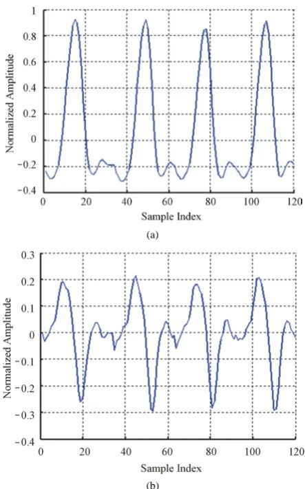
is normally quantized using a predefined number of bits. If the calculated difference between the current sample and the predicted value of the current sample is too large to be represented by the number of bits chosen for quantization, then data loss occurs. For this reason DPCM is normally considered to be a nearly lossless coding scheme. Therefore, in order to keep the DPCM operation completely lossless, the output would need more predefined bits to guarantee that there will not be data loss. In [11], Jalaleddine showed that for ECG signals, a first order linear predictor (DPCM) yields bet-ter results compared to LP models of higher orders. However, for other set of signals, a second order predic-tion model achieved best results. Figure 6 illustrates the ROI signal before and after DPCM.5.3. Compression of NonRoI Part Using DWT
As it is mentioned before, the NonRoI part is compressed using DWT-based compression technique. For all signals considered through the paper, signals are decomposed up to the 6 levels using Daubitches “db6” wavelet filters. Then the wavelet coefficients are thresholded, quantized and coded using run-length coding technique. The appro- ximation and details coefficients obtained by wavelet transformation must be quantized for the purpose of compression. The quantization process on the subbands of the ECG signal gives a small number of bits (short codewords) to represent the small numbers when they mostly occur and a larger number of bits (long code-
(a)
(b)
Figure 6. The ROI signal before and after DPCM; (a) The original signal (b) After DPCM.
words) to represent the less probable large numbers. For the run-length coding of the thresholded wavelet coeffi-cients of NonRoI part, each coefficient is represented in the forum of (counts, values). Then, each non-negative value is represented by “1” concatenated with nbitsNo- nRoI binary representation of that value and each nega- tive value is represented by “0” concatenated with nbits- NoRoI binary representation of that value. Here, nbits- NonRoI is determined such that the absolute value of the maximum thresholded wavelet coefficient is represented correctly. Consequently, counts are again run-length coded.
6. Data Packetization Process
[image:8.595.312.534.82.438.2]The second part of the header (Header2) packetize the number of bits required for representing the length of RoI residuals (Len_of_RoI), the value of the first sample, the number of bits for RoI residual (nbitsRoI) as shown in
Table 4. Before quantizing the residuals of the theRoI part, each residual element is multiplied by a scale factor of value 100. The required number of bits necessary to represent each element of the scaled e n
( )
depends mainly on the maximum value of e n( )
.6.1. Packtization of Transmitted Signal
Before quantizing the DWT coefficient of the NonRoI part, each coefficient is multiplied by a scale factor of value 100. The third part of the header (Header3) pack- etize the number of bits required for representing the NonRoI scaled DWT coefficients. In this case, the cod- ing process using run-length algorithm is applied twice. The first, results in values and counts of the scaled DWT coefficients. The required number of bits necessary to represent each value depends mainly on the maximum absolute value the scaled DWT coefficient. The Matlab function dec2bin is adopted for determining nbitsvalue. This function is also used to define the number of bits required to represent the number of these values (nbitsv- length). The resulting counts vector may have too many successive zeros. So, another run-length coding round for counts is adopted. This results in values and counts of counts. Thus we have to define the number of bits re-
Table 3. The construction of the first part of the header (Header1).
bits assigned for the number of T-waves 4-bits
bits assigned for the number of U-waves 4-bits
bits assigned for the number of PT-waves 4-bits
bits assigned for the number of QRS-waves 4-bits
Table 4. The construction of the second part of the header (Header2).
bits assigned for the length of
RoI residuals (Len_of_RoI) 8-bits
bits assigned for the first sample 10 bits + 1 sign bit
bits assigned for each RoI residual (nbitsRoI) 5 bits + 1 sign bit
quired for representing the length and the value of values of the scaled DWT coefficients, together with the value and count of their counts. The last count value that re- presents the number of zeros at the end of scaled DWT coefficients vector is high; thus it will be represented by more bits. Table 5 illustrates the number of bits assigned for NonRoI coded DWT coefficient. The fourth part of the header (HeaderW) contains the start and end indices of all ECG waves except the isoelectric waves; where each is represented by 11-bits (See the formula in the bottom).
Following the four header parts, the binary stream of the coded RoI residuals and the binary stream of the coded DWT coefficients are packetized consequently.
Table 6 summarizes the bit allocation, which is trans- mitted (stored) for every ECG signal block. The gray areas in the table denote the parameters that are not al- ways transmitted.
6.2. Illustrative Example of Packetization Process
To illustrate the packetization process, consider the above mentioned ECG signal (1460 samples from record 103). The signal contains 5 T-waves, 5 U-waves, 5 P- waves, and 4 QRS-waves. So, the binary stream of the first part of the header is Header1 = [0101 0101 0101 0100].
The signal also has 120 RoI residuals and a first sam- ple of value −0.237 The absolute value of the maximum element of the RoI residual is 30, so nbitsRoI = 6-bits. Thus, the binary stream of the second part of the header is Header2 = [01111000 10100010 00111100110 11110 000011110]. For the considered signal the number of
Table 5. Number of bits assigned for scaled NonRoI DWT coefficient (Header3).
Parameter Bits assigned for each Value Length
Values of coded DWT Coefficients
(nbitsvalue, nbitsvlength) 10-bits 7-bits
Count-value of coded DWT
(nbitscount-value, nbitscvlength) 7-bits 5-bits
Count-count of coded DWT
(nbitscount-count, nbitscclength) 5-bits 5-bits
Last count-value (nbitslast) 11-bits
(
)
(
)
(
)
(
)
(
)
(
)
(
)
- - -
-- - -
-- - -
-1 1 Num of Twaves Num of Twaves
1 1 Num of Twaves Num of Twaves
1 1 Num of Twaves Num of Twaves
1 1
HeaderW STwave , ETwave , , STwave , ETwave
SUwave , EUwave , , SUwave , EUwave
SPwave , EPwave , , SPwave , EPwave
SQwave , EQwave , , S
=
NonRoI samples is 1340. Among them, 318 samples re- present the T-waves, 165 samples representing the U- waves, 190 samples representing the P-waves and 667 samples representing the isoelectric-waves. When wave- let transformed using “db6” up to the 6th level, 1403 wavelet coefficients result. These wavelet coefficients are thresholded using 0.0485 threshold level, where those less than this value are set to zero. This level is calcu- lated using the energy packing efficiency principle de- scribed in [18]. As a result of this step, only 80 coeffi- cients from the 1403 wavelet coefficients are non-zeros
Table 6. The packetized bit stream of the compressed signal.
Header1 16-bits
Header2 25-bits
Header3 49-bits
HeaderW 11-bits * length of HeaderW
Bit stream of RoI 6 bits * length of RoI
Bit stream of NonRoI
9 bits * length of coded values vector + 7 bits * length of count values vector + 5 bits * length of count counts vector+
11 bits
and the remaining 1323 coefficients are zeros. However these zeros are distributed between the non-zero coeffi- cients. Using the run-length encoding, all the wavelet coefficients are grouped into 81 values with 81 counts. Thus, the 1403 wavelet coefficients are coded to 162 values and counts.
[image:10.595.53.541.402.637.2]Table 7 includes the 162 run-length codes of the NonRoI wavelet coefficients. In this table the wavelet coefficient of value −231 with count zero means that there are no zeros between this coefficient and the pre- ceding coefficient (−225). However, the wavelet coeffi- cient of value 74 with count 5 means that there are 5 ze- ros between this coefficient and the preceding coefficient (−213). Investigations of Table 7 reveal that, the counts have many repeated successive zeros. Consequently, the run-length method is adopted once again for counts vec- tor. As a result, the 81 counts are coded into 23 counts_ values and 23 counts_counts. Moreover the values of the resulting representation are much smaller than that of counts. Thus, the 1403 wavelet coefficients are coded by 81 coefficient values, 23 counts values and 23 counts counts. Table 8 includes the run-length coding of the coefficients counts; which is counts_counts and counts_ values. The last counts_values (1105) represents the
Table 7. The run-length codes of the NonRoI wavelet coefficients.
values −225 −226 −226 −226 −225 −225 −231 −209 −265 −76 −46 −77
counts 0 0 0 0 0 0 0 0 0 0 0 0
values −79 −53 −174 −188 −163 −185 −194 −161 −222 −232 −223 −271
counts 0 0 0 0 0 0 0 0 0 0 0 0
values −216 −282 −204 −249 −228 −206 −213 74 55 −20 −50 −39
counts 0 0 0 0 0 0 0 5 0 0 0 0
values 26 −17 28 −14 33 −15 13 −30 −8 29 −10 −28
counts 0 0 3 0 0 0 0 0 1 1 0 2
values −12 21 −31 62 −78 67 −67 44 −19 −9 −12 16
counts 1 7 0 0 0 0 0 0 6 0 0 1
values 19 −10 13 −10 11 −10 8 10 −10 12 10 −8
counts 0 0 0 2 3 0 0 4 2 6 10 0
values 8 −7 −7 8 11 −8 −9 −8 0
[image:10.595.61.540.668.737.2]counts 5 0 16 7 2 15 11 107 1105
Table 8. The run-length codes of the counts.
counts_counts 31 6 5 0 1 0 0 6 2 3 0 2
counts_values 5 3 1 1 2 1 7 6 1 2 3 4
counts_counts 0 0 0 1 1 0 0 0 0 0 0
number of zeros at the end of the thresholded NonRoI- coefficients. In fact this value is the maximum value of the vector counts_values and needs 11 bits for binary representation. Excluding this value from vector counts_ values yields that the maximum value of the remaining elements is 107, so only 7 bits is enough for representing each element in counts_values. Thus, Header3 is [(10, 81) (7, 23) (5, 22) 11] which is equivalent to [1010 1010001 0111 10111 0101 10110 1011].
The fourth part of the header is devoted to the binary stream of the start and end locations of the 5 T-waves, 5 U-waves, 5 P-waves, and 4 QRS-waves. These locations are respectively at the indices [1 331 635 936 1240 89 387 689 992 1299 126 423 722 1035 1337 153 455 757 1069 1369 192 501 803 1108 1411 225 536 837 1142 1460 252 563 864 1168 285 591 892 1195]. Represen- ting each index by 11-bits, yield HeaderW =
[00000000001 00101001011
01001111011 ··· 01101111100 10010101011].
Following the transmission of the four header parts, the binary stream of the scaled RoI residuals is transmit- ted. The number of these elements is 120 and each is represented by 6 bits including the sign bit. Thus the 120 residual elements are represented by a binary stream of length 720 bits. The first 10 residual elements after scal- ing are [0 −3.0 −2.0 −1.0 2.0 3.0 5.0 9.0 15.0 19.0] and the corresponding binary stream is [100000 000011 000010 000001 100010 100011 100101 101001 101111 110011].
Following the transmission of the RoI residuals, the binary stream of the coded NonRoI part is transmitted. Adding the 11-bits required for the last counts value (1105), a sum of 165 bits represents counts-values vector. For counts-counts vector, the maximum element is 31, so 5 bits are enough to represent each element. Conse- quently 110 bits represents the counts-counts vector. Thus, 275 bits are needed after run-length encoding of counts vector. The maximum absolute value of the values vector is 282. This value is represented by 9 bits plus one more bit for sign. The last element of the vector values is zero and the remaining 80 elements need 800 bits for binary representation. Summing up all together, the 1403 thresholded DWT coefficients are represented by 1082 bits.
7. Numerical Results
In this section, the performances of the proposed compres- sion algorithm is presented and will be compared with other known compression algorithms. Records from MIT- BIH Arrhythmia database is used for evaluating the pro- posed compression algorithm. The performance of com- pression algorithms is tested by means of the quantitative performance measures; namely, in terms of the compres- sion ratio and the distortion metrics. The compression
ratio (CR) is defined as the ratio of the number of bits representing the original signal to the number required for representing the compressed signal. So, it can be cal- culated from:
HW RoI NonRoI
c
Lsb CR
N +N +N
= (6)
where, bc is the number of bits representing each orig- inal ECG sample. For MIT-BIH database, bc is 11 bits.
HW
N , NRoI, and NNonRoI are the number of bits repre- senting HeaderW, RoI stream and NonRoI stream re- spectively. It should be noted that NH1,NH2 and NH3 are the lengths of the binary streams representing Head- er1, Header2 and Header3. They are not included in (6), since they are fixed and send to the receiver once. To be able to compare different compression algorithms, it is imperative that an error criterion is defined such that it will measure the ability of the reconstructed signal to preserve the relevant diagnostic information. The distor- tion resulting from the ECG processing is frequently measured by the percent root-mean-square difference (PRD).
( ) ( )
(
)
( )
2 1 2 1 % 100 N n N nx n x n
PRD x n = = − =
∑
×∑
(7)where, x n
( )
is the original signal, x n( )
is the recon- structed signal and N is the length of the window over which the PRD is calculated.7.1. Illustrative Example of Compression Algorithm
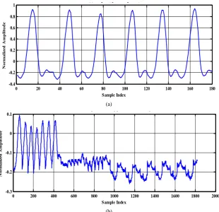
As an illustrative example, consider the compression of 2000 samples extracted from record 100 of MIT-BIH da- tabase. Thus, these samples are represented by 22000 bits. The signal is segmented into RoI and NonRoI parts. Con- sidering the RoI part to include the QRS-waves and the NonRoI part to include the remaining waves, the length of RoI part is 180 samples and that of NonRoI part is 1820 samples as shown in Figure 7. In this case, the R- peaks locations and the QRS starts and ends locations are required to be determined. Those are: R-peaks = [266 577 878 1182 1484 1796], QRS-starts = [252 563 864 1168 1470 1781] and QRS-ends = [285 591 892 1195 1497 1812]. Each QRS start and end value is represented by 11-bits yielding NHW=132-bits. The RoI part is de- correlated using DPCM and this yields first-sample = −0.2375 and the residual waveform shown inFigure 8(a). The NonRoI part is wavelet transformed up to the 6th level using Daubechies (db6) wavelet and the resulting waveform coefficients (1884) are shown in Figure 8(b).
(a)
[image:12.595.143.454.83.383.2](b)
Figure 7. The RoI part before and after DPCM. (a) RoI part (QRS-complexes); (b) NonRoI (remaing part of the ECG signal).
(a)
(b)
Figure 8. The RoI part after DPCM and the wavelet coefficients of the Non-RoI part. (a) RoI part after DPCM; (b) Wavelet coefficients of NonRoI part.
0 20 40 60 80 100 120 140 160 180 -0.4
-0.2 0 0.2 0.4 0.6 0.8 1
(a) o pa t (Q S co p e es)
S ample Index
N
or
mal
iz
e
d
A
mp
li
tu
d
e
0 200 400 600 800 1000 1200 1400 1600 1800 2000 -0.3
-0.2 -0.1 0 0.1
( ) p ( g p g )
S ample Index
N
or
mal
iz
e
d
A
mp
li
tu
d
e
0 20 40 60 80 100 120 140 160 180
-0.4 -0.3 -0.2 -0.1 0 0.1 0.2 0.3
( ) p
S ample Index
N
or
mal
iz
ed
A
mp
li
tu
d
e
0 200 400 600 800 1000 1200 1400 1600 1800 2000 -2
-1.5 -1 -0.5 0 0.5
S ample Index
N
or
mal
iz
ed
A
mp
li
tu
d
[image:12.595.124.471.415.708.2]energy of the NonRoI part is reserved. The maximum absolute value of the residuals of the RoI part after scal- ing and rounding is 15. Thus, length of the RoI stream is
RoI
N
= 900 bits. The wavelet coefficients whose abso- lute values are less than the resulting threshold level (0.0592) are set to zero. As a result, among the 1884 waveform coefficients, only 84 coefficients are non-zero. However, they are distributed between the waveform coefficients.After running the first round run-length coding algo- rithm, 85 values and 85 counts results. Concerning the 85 values, the maximum absolute value is 185. Thus each value is represented by 9-bits including the sign bit and the binary stream of the values is of length 765 bits. Af-ter the second round of run-length coding algorithm on the 85 counts, the following 20 values and 20 runs result respectively;
Counts_values = [5 6 3 1 1 1 2 7 2 6 3 2 6 2 3 1 12 10 48 1678]
Counts_counts = [0 0 0 1 0 0 0 0 0 0 3 1 8 0 0 1 3 1 8 39]
The maximum value of the first 19 counts-values is 48 and each can be represented by 6-bits yielding 114-bits for representing the counts-values stream. The last counts-values is 1678 which is represented by 11-bits. Similarly, the maximum value of the first counts-counts is 8 and each can be represented by 4-bits yielding 76- bits for representing the counts-values stream. The last counts-counts is 39 which is represented by 6-bits. Sum- ming all together, NNonRoI=207-bits and
HW RoI NonRoI 1239-bits
N +N +N = . Thus, from Equation
(6), the compression ratio is CR=17.76.
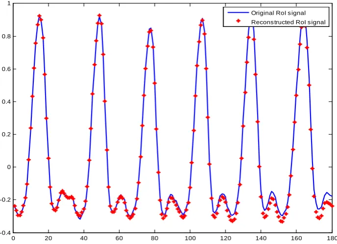
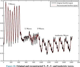
Reconstructing the ECG signal from the header and the binary streams representing the RoI and NonRoI parts follows reverse processes. This is namely, decoding of header, RoI and NonRoI streams. Then, the RoI and NonRoI parts are reconstructed using inverse DPCM and inverse DWT respectively. The QRS-starts, QRS-ends and the reconstructed RoI and NonRoI parts are used to reconstruct the ECG signal. Figure 9 illustrates the orig- inal and reconstructed RoI part of the signal. This figure shows that the original and the reconstructed QRS-waves are almost identical. Figure 10 illustrates the original and reconstructed T-, P-, U- and isoelectric waves together with the reconstruction error of the NonRoI part. Figure 11 illustrates original and the reconstructed ECG wave- forms results from inserting the RoI and NonRoI parts in their prober positions.
7.2 Effect of Selecting the Wavelet Family
[image:13.595.126.470.471.720.2]The Wavelet Toolbox™ software includes a large num- ber of wavelets that you can be used for ECG signal compression. Examples include: orthogonal wavelets (Daubechies’ and Symlets wavelets) and biorthogonal wavelets. The choice of wavelet is dictated by the signal characteristics and the nature of the application. The wavelet families adopted in this paper are listed in Table 9. Table 10 depicts the wavelets used for testing the ef- fect of varying the wavelet filters on the compression performances. Figures 12 and 13 illustrate the dependence of the CR and PRD on the adopted wavelet filters. These
Figure 9. The original and reconstructed RoI part (QRS waves).
0 20 40 60 80 100 120 140 160 180 -0.4
-0.2 0 0.2 0.4 0.6 0.8 1
0 200 400 600 800 1000 1200 1400 1600 1800 2000 -0.3
-0.25 -0.2 -0.15 -0.1 -0.05 0 0.05 0.1
Original NonRoI signal Reconstructed NonRoI signal
U-Waves P-Waves
[image:14.595.139.456.88.352.2]isoelectric-Waves T-Waves
[image:14.595.63.542.380.736.2]Figure 10. Original and reconstructed T-, P-, U- and isoelectric waves.
Table 9. Wavelet families adopted for ECG signal compression.
Wavelet Family
Example Short Name Name
“db” Daubechies wavelets
In dbN wavelets N refers to the number of vanishing moments.
“sym” Symlets wavelets
In symN wavelets, N is the number of vanishing moments (symN is more
symmetrical than dbN)
“bior” Biorthogonal wavelets
In Biorthogonal wavelets, the pair (Nr .Nd) indicates the orders of the filters. Nr for
Table 10. Daubechies, Symlets and Biorthogonal filters used in the ECG compression.
Filter number 1 2 3 4 5 6 7 8 9 10
Daubechiesfilter name db 1 db 2 db 3 db 4 db 5 db 6 db 7 db 8 db 9 db 10
Symlets filter name sym 2 sym 3 sym 4 sym 5 sym 6 sym 6 sym 7 sym 8
Biorthogonal filter name bior 1.1 bior 1.3 bior 1.5 bior 2.2 bior 2.4 bior 2.6 bior 2.8 bior 3.1 bior 3.3 bior 3.5
Filter number 11 12 13 14 15 16 17 18 19 20
Daubechiesfilter name db 11 db 12 db 13 db 14 db 15 db 16 db 17 db 18 db 19 db 20
[image:15.595.151.447.481.720.2]Biorthogonal filter name bior 3.7 bior 3.9 bior 4.4 bior 5.5 bior 6.8
Figure 11. Original and reconstructed ECG signal and reconstruction error.
Figures 12. Dependence of the CR on the adopted wavelet filters.
0 200 400 600 800 1000 1200 1400 1600 1800 2000 -0.5
0 0.5 1
original signal
0 200 400 600 800 1000 1200 1400 1600 1800 2000 -0.5
0 0.5 1
reconstructed signal
0 200 400 600 800 1000 1200 1400 1600 1800 2000 -0.1
-0.05 0 0.05 0.1
difference between original and reconstructed signals
0 2 4 6 8 10 12 14 16 18 20
8 9 10 11 12 13 14 15 16 17
Filter number
CR
Daubechies filters family
Figures 13. Dependence of the PRD% on the adopted wavelet filters.
figures show that as the filters order increase, the CR increases. However, this increases the compression errors. They also show that Daubechies’ and Symlets families outperforms biorthogonal family; where higher CRs and lower reconstruction errors result.
7.3. Comparison with Other Methods
In technical literatures, many interesting ECG signal compression algorithms have been introduced. In this section the result of several experiments of the proposed method are compared with other ECG compression algo- rithms already realized [12-21]. In addition, the ECG signals used should be sampled with the same sampling rate and each sample is quantized by the same number of bits. The proposed algorithm was tested and evaluated using actual data from MIT-BIH arrhythmia database; where the sampling rate is 360 Hz, and the resolution is 11-bit. The performance of the algorithm is measured and compared with other methods used the same records according to its PRD and CR for each experiment. The dataset adopted consist of 10 seconds of data from records 100 and 117. Tables 11 and 12depict the com- parison of performance results of CR and PRD with those in literature for record 117 and 100 respectively. From this table, it can be deduced that the proposed me- thod got higher compression ratios compared to the other wavelet transformation techniques. Moreover, the pro- posed method possesses lower PRD. This is due to the fact that the proposed method is combined approach of
Table 11. Comparison with other methods in compressing record 117.
Algorithm PRD (%) CR
Donoho [12], 1995 3.90 8.0:1
Djohan et al. [13], 1997 3.90 12.5 Hilton [14], 1997 2.60 14.9
Al-Shrouf et al. [15], 2003 5.30 11.6:1 Tohumoglu and Sezgin [16], 2007 5.83 14.9:1
Boukhennouf et al. [17], 2009 2.43 14.3:1
Abo-Zahhad et al. [18], 2011 1.60 19.2:1 Hossain and Amin [19], 2011 2.50 15.1:1
Chouakri et al. [20], 2013 4.75 14.01 Proposed Algorithm-Daubechies 2.81 15.6:1
Proposed Algorithm-Symlets 2.90 13.69:1
Proposed Algorithm-Biorthogonal 2.82 14.48:1
lossy compression (DPCM) and lossless compression (DWT) techniques.
8. Conclusions
This paper presents a hybrid technique for the compres- sion of ECG signals based on DWT and exploiting the correlation between ECG samples; where lossless com-
0 2 4 6 8 10 12 14 16 18 20
2.3 2.4 2.5 2.6 2.7 2.8 2.9 3
Filter number
P
RD %
[image:16.595.136.467.83.353.2] [image:16.595.309.537.407.634.2]Table 12. Comparison with other methods in compressing record 100.
Algorithm PRD (%) CR
Istepanian et al. OZWC [21], 2001 0.5778 (NRMSE) 8.16:1 Istepanian et al. WHOSC [21], 2001 1.7399 (NRMSE) 17.5:1 Chouakri et al. [20], 2013 19.35 13.8:1 Proposed Algorithm-Daubechies 2.77 16.2:1
Proposed Algorithm-Symlets 2.78 14.7:1
Proposed Algorithm-Biorthogonal 2.82 15.1:1
pression is adopted for clinically relevant parts and lossy compression is adopted for other parts. The ECG signal is segmented into P-waves, QRS-complexes, T-waves, U-waves and isoelectric waves. They are grouped into Region of Interest (RoI) and Non Region of Interest (NonRoI) parts. For a given fixed bit budget, more bits are devoted to representing RoI parts, while allowing other parts to suffer larger distortion. For this purpose the cor- relation between the successive samples of the ROI part has been utilized by adopting DPCM approach and the NonRoI part is compressed using DWT, thresholding and coding techniques. Compression is then achieved by se- lecting a subset of the most relevant coefficients which afterwards are efficiently coded. Illustrative examples are given to demonstrate thresholding based on energy pac- king efficiency strategy, coding of DWT coefficients and data packetizing. The principal advantages of the pro- posed approach are: 1) the deployment of different com- pression schemes to compress different ECG parts to reduce the correlation between consecutive signal sam- ples; and 2) getting high compression ratios with accept- able reconstruction signal quality compared to the re- cently published results.
The performances of the proposed compression algo- rithm are evaluated and compared with other known compression algorithms adopting records from MIT-BIH Arrhythmia database. The quality of the proposed com- pression algorithm is tested in terms of the compression ratio and the PRD distortion metrics using 10 seconds of data from records 100 and 117. The obtained results re- vealed that the proposed method possesses higher com- pression ratios and lower PRD compared to the other wavelet transformation techniques. This is due to the fact that the proposed method is a combined approach of los- sy compression (DPCM) and lossless compression (DWT) techniques.
REFERENCES
[1] P. S. Addison, “Wavelet Transforms and the ECG: A Review,” Physiological Measurement, Vol. 26, No. 5,
2005, pp. 155-199.
http://dx.doi.org/10.1088/0967-3334/26/5/R01
[2] S. Olmos, M. Millán, J. García and P. Laguna, “ECG Data Compression with the Karhunen-Loève Transform,” Proceedings of Computers in Cardiology, Indianapolis, IEEE Press, Piscataway, 1996, pp. 253-256.
[3] B. R. S. Reddy and I. S. N. Murthy, “ECG Data Com- pression Using Fourier Descriptions,” IEEE Transactions on Biomedical Engineering, Vol. 33, No. 4, 1986, pp. 428-434. http://dx.doi.org/10.1109/TBME.1986.325799
[4] N. Ahmed, P. J. Milne and S. G. Harris, “Electrocardio- graphic Data Compression Via Orthogonal Transforms,” IEEE Transactions on Biomedical Engineering, Vol. BME-22, No. 6, 1975, pp. 484-487.
http://dx.doi.org/10.1109/TBME.1975.324469
[5] J. H. Husøy and T. Gjerde, “Computationally Efficient Subband Coding of ECG Signals,” Medical Engineering & Physics, Vol. 18, No. 2, 1996, pp. 132-142.
http://dx.doi.org/10.1016/1350-4533(95)00028-3
[6] C. P. Mammen and B. Ramamurthi, “Vector Quantization for Compression of Multichannel ECG,” IEEE Transac- tions on Biomedical Engineering, Vol. 37, No. 9, 1990, pp. 821-825. http://dx.doi.org/10.1109/10.58592
[7] J. Chen, S. Itoh and T. Hashimoto, “ECG Data Compres- sion by Using Wavelet Transform,” IEICE Transactions on Information and Systems, Vol. E76-D, No. 12, 1993, pp. 1454-1461.
[8] D. Haugland, J. Heber and J. Husøy, “Optimization Algo- rithms for ECG Data Compression,” Medical & Biologi- cal Engineering & Computing, Vol. 35, No. 4, 1997, pp. 420-424. http://dx.doi.org/10.1007/BF02534101
[9] R. Nygaard, G. Melnikov and A. K. Katsaggelos, “Rate Distortion Optimal ECG Signal Compression,” Proceed- ings of International Conference on Image Processing, Kobe, 24-28 October 1999, pp. 348-351.
[10] P. de Chazal, S. Palreddy and W. J. Tompkins, “Auto- matic Classification of Hear-Beats Using ECG Morphol- ogy and Heartbeat Interval Features,” IEEE Transactions on Biomedical Engineering, Vol. 51, No. 7, 2004, pp. 1196-1206.
http://dx.doi.org/10.1109/TBME.2004.827359
[11] S. Jalaleddine, C. Hutchens, R. Strattan and W. Coberly, “ECG Data Compression Techniques—A Unified Ap- proach,” IEEE Transactions on Biomedical Engineering, Vol. 37, No. 4, 1990, pp. 329-343.
http://dx.doi.org/10.1109/10.52340
[12] D. L. Donoho, “Denoising by Soft-Thresholding,” IEEE Transactions on Information Theory, Vol. 41, No. 3, 1995, pp. 613-627. http://dx.doi.org/10.1109/18.382009
[13] A. Djohan, T. Q. Nguyen and W. J. Tompkins, “ECG Com- pression Using Discrete Symmetric Wavelets Transform,” IEEE—EMBC and CMBEC, Vol. 14, No. 2, 1997, pp. 167-168.
[14] M. L. Hilton, “Wavelet and Wavelet Packet Compression of Electrocardiograms,” IEEE Transactions on Biomedi- cal Engineering, Vol. 44, No. 5, 1997, pp. 394-402.
http://dx.doi.org/10.1109/10.568915
[image:17.595.59.286.111.229.2]Novel Compression Algorithm for Electrocardiogram Signals Based on the Linear Prediction of the Wavelet Coefficients,” Digital Signal Processing, Vol. 13, No. 4, 2003, pp. 604-622.
http://dx.doi.org/10.1016/S1051-2004(02)00031-3
[16] D. Tohumoglu and K. Erbil Sezgin, “ECG Signal Com-pression by Multiiteration EZW Coding for Different Wavelets and Thresholds,” Computers in Biology and Medicine, Vol. 37, No. 2, 2007, pp. 173-182.
http://dx.doi.org/10.1016/S1051-2004(02)00031-3
[17] N. Boukhennoufa, K. Benmahammed, M. A. Abdi and F. Djeffal, “Wavelet-Based ECG Signals Compression Us- ing SPIHT Technique and VKTP Coder,” International Conference on Signals, Circuits and Systems, Medenine, 6-8 November 2009, pp. 1-5.
[18] M. Abo-Zahhad, S. M. Ahmed and A. Zakaria, “ECG Signal Compression Technique Based on Discrete Wave-let Transform and QRS-Complex Estimation,” Signal
Processing—An International Journal (SPIJ), Vol. 4, No. 2, 2011, pp. 138-160.
[19] M. S. Hossain and N. Amin, “ECG Compression Using Sub-Band Thresholding of the Wavelet Coefficients,” Australian Journal of Basic and Applied Sciences, Vol. 5, No. 5, 2011, pp. 739-749.
[20] S. A. Chouakri, O. Djaafri1 and A. Taleb-Ahmed, “Wave- let Transform and HUFFMAN Coding Based Electrocar- diogram Compression Algorithm: Application to Tele- cardiology,” 24th IUPAP Conference on Computational Physics, Journal of Physics Conference Series, Vol. 454, No. 1, 2013, pp. 1-16.