Biometric cattle identification approach
based on Weber's local descriptor and
AdaBoost classifier
Gaber, T, Tharwat, A, Hassanien, AE and Snasel, V
http://dx.doi.org/10.1016/j.compag.2015.12.022
Title
Biometric cattle identification approach based on Weber's local descriptor
and AdaBoost classifier
Authors
Gaber, T, Tharwat, A, Hassanien, AE and Snasel, V
Type
Article
URL
This version is available at: http://usir.salford.ac.uk/id/eprint/52086/
Published Date
2016
USIR is a digital collection of the research output of the University of Salford. Where copyright
permits, full text material held in the repository is made freely available online and can be read,
downloaded and copied for noncommercial private study or research purposes. Please check the
manuscript for any further copyright restrictions.
Biometric Cattle Identication Approach Based on
Weber's Local Descriptor and AdaBoost Classier
Tarek Gabera,b,c,1,∗, Alaa Tharwatc,d, Aboul Ella Hassanienc,e, Vaclav Snaself aFaculty of Computers and Informatics, Suez Canal University, Ismailia, Egypt
bIT4Innovation, VSB-TU of Ostrava, Ostrava, Czech Republic cScientic Research Group in Egypt (SRGE), http://www.egyptscience.net
dFaculty of Engineering, Suez Canal University, Ismailia, Egypt eFaculty of Computers and Information, Cairo University, Egypt
fFEECS, Dept. of Computer Science and IT4Innovations, VSB-TU of Ostrava, Czech Republic
Abstract
In this paper, we proposed a new and robust biometric-based approach to
iden-1
tify head of cattle. This approach used the Weber Local Descriptor (WLD) to
2
extract robust features from cattle muzzle print images (images from 31 head of
3
cattle were used). It also employed the AdaBoost classier to identify head of
4
cattle from their WLD features. To validate the results obtained by this
clas-5
sier, other two classiers (k-Nearest Neighbor (k-NN) and Fuzzy-k-Nearest
6
Neighbor (Fk-NN)) were used. The experimental results showed that the
pro-7
posed approach achieved a promising accuracy result (approximately 99.5%)
8
which is better than existed proposed solutions. Moreover, to evaluate the
re-9
sults of the proposed approach, four dierent assessment methods (Area Under
10
Curve (AUC), Sensitivity and Specicity, accuracy rate, and Equal Error Rate
11
(EER)) were used. The results of all these methods showed that the WLD along
12
with AdaBoost algorithm gave very promising results compared to both of the
13
k-NN and Fk-NN algorithms.
14
Keywords: Cattle identication, Weber Local Descriptor (WLD), k-Nearest Neighbor, Fuzzy-k-Nearest Neighbor, Muzzle print images, dimensionality reduction, feature extraction, AdaBoost classier, Animal identication
∗Corresponding author
1. Introduction
15
Cattle identication and traceability are very crucial to control safety policies
16
of animals and management of food production. Many international
organiza-17
tions, e.g. food safety and world animal health, have formally recognized the
18
signicant values of the development of the animal identication and
traceabil-19
ity systems and they further actively promoted for these systems (Schroeder and
20
Tonsor, 2012). Such values include (a) controlling the widespread of the animal
21
diseases by identifying and detecting infected animals, (b) reducing losses of
live-22
stock producers by controlling the diseases, (c) decreasing the government cost
23
by the control, intervention, and eradication of the outbreak diseases (Bowling
24
et al., 2008). Therefore, especially after the discovery of the Bovine Spongiform
25
Encephalopathy (BSE), advanced animal identication and traceability systems
26
were evolved and deployed by big beef exporters and have been increasingly used
27
by ranked beef importing countries (Schroeder and Tonsor, 2012).
28
Marchant (2002) reported that animal identication can be achieved using
29
many dierent methods which could be classied as mechanical, electronic, and
30
biometric. The mechanical class includes methods such as ear notching, ear tags,
31
branding, and tattoos. Nonetheless, as reported in (Shadduck and Golden, 2002;
32
Allen et al., 2008), the mechanical-based identication suers from a number of
33
limitations. The ear notching method is not suitable for large-scale identication
34
systems. The ear tag methods (metal clips and plastic tags) are not so expensive,
35
but they may cause animal infections (Allen et al., 2008). The branding and
36
tattoo methods are not achieving a relatively good accuracy as in one herd, all
37
head of cattle are identically branded. Thus, they are not useful to uniquely
38
dierentiate between various head of cattle in the same herd. In addition, these
39
methods take more time than other modern techniques (Shadduck and Golden,
40
2002).
41
Animal identication systems based on electronic methods (Marchant, 2002;
42
Shanahan et al., 2009) used Radio Frequency Identication (RFID) to identify
43
animals. These methods are mainly based on attaching two devices with the
animals. One device contains a unique identication number and the other is the
45
reading device which reads and interprets animals code (the unique identication
46
number). When a code is scanned, the reading device sends it to a database for
47
future actions. The main limitation of this method is that the attached devices
48
may get lost, removed, or damaged (Marchant, 2002).
49
The third method is the biometric-based animal identication (Shadduck
50
and Golden, 2002; Jiménez-Gamero et al., 2006; Rusk et al., 2006; Corkery
51
et al., 2007; Allen et al., 2008; Barry et al., 2008; Gonzales Barron et al., 2008;
52
Rojas-Olivares et al., 2011; Adell et al., 2012). Similar to biometric-based
hu-53
man identication, a number of biometric animal have proposed to uniquely
54
identify animals. Retina-based identication systems (Rusk et al., 2006; Allen
55
et al., 2008; Barry et al., 2008; Gonzales Barron et al., 2008; Adell et al., 2012)
56
depend on the retinal image recognition (RIR) which utilizes the fact that the
57
retina vessels of each head of cattle is a unique identier. DNA-based methods
58
(Jiménez-Gamero et al., 2006) were also proposed to identify meat products
59
that were produced from a given specic animal. Although this method, in case
60
of head of cattle, gives a higher identication rate than the other methods, it
61
is intrusive, and not cost-eective and it could last days or weeks to obtain the
62
identication result (Rusk et al., 2006). Other biometric-based methods include
63
animal facial recognition (Shadduck and Golden, 2002; Corkery et al., 2007) and
64
muzzle-based identication (Minagawa et al., 2002; Noviyanto and Arymurthy,
65
2012; Awad et al., 2013; Noviyanto and Arymurthy, 2013).
66
The muzzle-based animal identication is based on the fact that the muzzle
67
pattern or nose print of dierent animals of the same species are mostly unique
68
(Baranov et al., 1993; Gonzales Barron et al., 2008). Thus, it is concluded that
69
muzzle print is similar to a human's ngerprint. The muzzle-based approach is
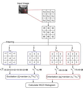
70
a very promising way for cattle identication as it can achieve a high accuracy
71
(e.g. 90.6% in (Noviyanto and Arymurthy, 2012)). Using this approach, there
72
is no need to attach or insert external parts within the animals. Moreover, it
73
complies with most countries legal rules.
74
In the muzzle-based identication system, extracting discriminative features
from the muzzle images is a very important step. Local invariant features are
76
good ones as they are robust against many challenges such as noise,
illumina-77
tion, transformation, rotation, and occlusion. There are two methods to extract
78
the local invariant features: sparse descriptor (Lowe, 1999) and dense descriptor
79
(Chen et al., 2010). In the former method, the interest points (keypoints), are
80
rst detected, then a local patch, around these keypoints, is constructed, and
81
nally invariant features are extracted. Scale Invariant Feature
Transforma-82
tion (SIFT) is considered one of the most well-known algorithms in the sparse
83
descriptor type (Lowe, 1999). In the dense descriptor-based methods, local
84
features are extracted from every pixel (pixel by pixel) over the input image.
85
Examples of this method include Local Binary Pattern (LBP) and Weber Local
86
Descriptor (WLD) (Ojala et al., 2002; Chen et al., 2010).
87
In this paper, a muzzle-based cattle identication approach was proposed.
88
This approach consists of three phases: feature extraction, feature reduction,
89
and classication. In the rst phase, the WLD algorithm was used to extract
90
local features. In the second phase, the Linear Discriminant Analysis (LDA)
91
technique was used to reduce the features and further to discriminate between
92
dierent images of various head of cattle. In the classication phase, three
93
classiers (AdaBoost, k-Nearest Neighbor (k-NN), and Fuzzy k-NN (Fk-NN))
94
were used to match between unknown cattle images and trained or labeled
95
images and then based on the highest accuracy results, the best classier was
96
recommended for the cattle identication system.
97
The rest of the paper is organized as follows. Section 2 summarizes the
re-98
lated work of the cattle identication system based on information technology.
99
Section 3 gives overviews of the techniques and methods used for the proposed
100
approach while Section 4 describes our proposed approach in detail.
Experimen-101
tal results and discussion are introduced in Section 5 and Section 6, respectively.
102
Finally, conclusions are summarized in Section 7.
2. Related Work
104
There are a number of the muzzle-based cattle identication approaches
105
(Minagawa et al., 2002; Noviyanto and Arymurthy, 2012; Awad et al., 2013;
106
Noviyanto and Arymurthy, 2013; Tharwat et al., 2014). These approaches used
107
dierent techniques to extract biometric features from muzzle images.
Mina-108
gawa et al. (2002) proposed the rst cattle identication approach in which
109
the joint pixels of the grooves were extracted by applying the image processing
110
techniques, i.e. ltering, binary transforming, and thinning. The identication
111
was then achieved by matching the joint pixels of a cattle image to the others
112
or to itself. The experiments of their proposed approach were conducted on a
113
database of 43 head of cattle and achieved minimum matching scores at 12%
114
and maximum scores at 60%. The results also showed that the identication
115
accuracy was around 30%.
116
The Speed Up Robust Features (SURF) and its variant (U-SURF) feature
ex-117
traction techniques were used in (Noviyanto and Arymurthy, 2012). Noviyanto
118
et al. used 15 muzzle print images in their experimental scenarios (10 images
119
were used in the training phase, and ve images were used in the testing phase).
120
The SURF-based method was found superior to U-SURF-based one as the
for-121
mer achieved 90% identication accuracy against rotation conditions.
122
Awad et al. (2013) used SIFT technique to detect the interesting points of
123
muzzle images for the purpose of cattle identication. To improve the
robust-124
ness of their proposed approach, they applied the RANdom SAmple Consensus
125
(RANSAC) algorithm along with the output of SIFT technique. In their
exper-126
iment, they used six images for each head of cattle and in total their database
127
includes 90 images (6×15 = 90). They achieved 93.3% accuracy of cattle
128
identication.
129
Also, Noviyanto and Arymurthy (2013) applied the SIFT technique to
muz-130
zle patterns lifted on paper in order to achieve cattle identication. To improve
131
the identication performance of their system, they also proposed a new
match-132
ing renement technique based on the keypoint of the orientation information.
They tested the proposed system using a database composed of 160 muzzle
im-134
ages left on papers and taken from 20 head of cattle. The achieved accuracy
135
results using SIFT only were equal to 0.0167 Equal Error Rate (EER) whereas
136
using SIFT along with the proposed new matching renement technique
mini-137
mized the EER to be 0.0028.
138
Tharwat et al. (2014) used the LBP technique for the feature extraction
139
phase of a muzzle-based cattle identication approach. The LBP was used as
140
it extracts robust texture features which are invariant to rotation and occlusion
141
of the images. They also used LDA to (a) address LBP high dimensionality
142
problem, and (b) discriminate between dierent classes, thus improving the
143
accuracy of their proposed system. For the identication phase, they tested
144
four dierent classiers (Nearest Neighbor, k-Nearest Neighbor (k-NN), Naive
145
Bayes, and Support Vector Machine (SVM)). The results showed that their
146
proposed approach achieved 99.5% identication accuracy.
147
3. Preliminaries
148
This section gives overviews of the techniques, algorithms, and methods used
149
in the design of the proposed approach.
150
3.1. Weber Local Descriptor (WLD)
151
The WLD technique is an image descriptor technique which describes an
152
image as a histogram of gradient orientations and dierential excitations (Chen
153
et al., 2010). It is originally inspired by Weber's Law where Ernst Weber, in the
154
19th century, observed that the ratio between an increment threshold and the 155
background intensity is constant and this can be formally expressed as follows:
156
∆I
I =k (1)
where∆I represents the increment threshold,Irefers to the initial intensity or 157
an image background, andk denotes the constant value even ifI is changing. 158
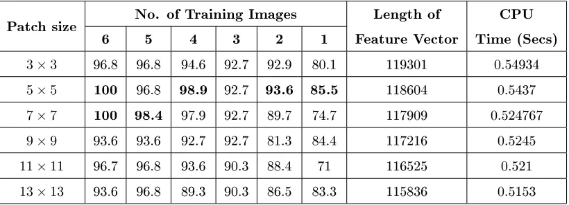
The fraction ∆I
In WLD algorithm, features are extracted from each pixel in an image. In
160
general, WLD algorithm consists of three steps, nding dierential excitations,
161
gradient orientations, and building the histogram. For each pixel in the input
162
image, the dierential excitation is rst computed and the gradient orientation
163
is then calculated to extract local features. Finally, a WLD histogram is built by
164
combining dierential excitation and gradient orientation for each pixel (Chen
165
et al., 2010). These steps are further explained below.
166
3.1.1. Dierential Excitation (ξ): 167
A dierential excitation (ξ) of a pixel is calculated as follows: 168
1. Calculating the dierence between the pixelxc (the center pixel) and its 169
neighbors using Equation (2) (Chen et al., 2010).
170
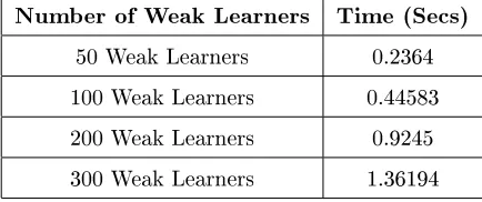
νs00=
p−1 X
i=0
(∆xi) = p−1 X
i=0
(xi−xc) (2)
where xi(i= 0,1, . . . , p−1) represents the intensity of the ith neighbors 171
of xc and prefers to the number of neighbors. An illustrative example, 172
inspired by the one in (Chen et al., 2010), is given in Figure 1 to show
173
how the dierential excitation is calculated. As shown in the gure, there
174
are eight neighbors to xc, where p = 8. To calculate the dierential
175
excitation and the orientation, four lters,f00, f01, f10, andf11 are used
176
to calculateν00
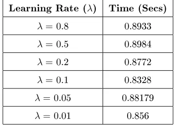
s , νs01, νs10, andνs11, respectively, where, νs00 represents the 177
dierence betweenxcand its neighbors as shown in Equation (2),νs01=xc, 178
νs10=x5−x1, andνs11=x7−x3.
179
2. Computing the ratio between the dierences,ν00
s , and the intensity of the current pixel,ν01
s =xc. This can be achieved using Equation (3).
Gratio(xc) =νs00/νs01 (3)
3. Applying the arc-tangent function on Gratio(.) to get the dierential
ex-180
citation of(xc), as shown in Equation (4).
ξ(xc) =Garctan[Gratio(xc)] =arctan
νs00/νs01
=arctan
"p−1 X
i=0
xi−xc xc
#
(4)
Dx0H Dx1H Dx2H
Dx3H
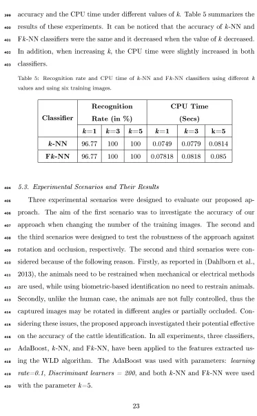
Dx4H
Dx5H
Dx6H
Dx7H DxcH
Input=Image
F1 F1 F1
F1 F1 F1 F1 -8
f00
F1
F1
f01
0 0 0
0 0 0
0 0
0
f10
-1 0 0
F1 0 0
0 0
0
f11
-1 0 0
0 0 F1
0
vs00 vs01 vs10 vs11
Excitation=DξH=arctan=Dνs00/νs01H Orientation=DφtH=arctan=Dνs11/νs10H
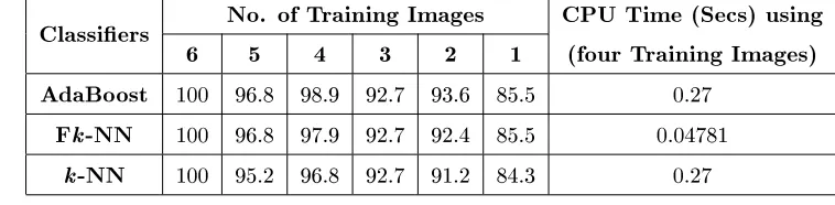
0
Calculate=WLD=Histogram
20 30 50 45 92 66 86 70 50
==-30-20F0-5F42F16F36F20=59 =xc=50 =66-30=36 =70-45=25
[image:9.612.145.467.202.546.2]Filtering
Figure 1: Illustration of the computation of the WLD algorithm.
3.1.2. Orientation (φt): 182
The orientation of a pixel (xc) is computed as follows: 183
the changes in the horizontal and vertical directions as follows:
θ(xc) =arctan
νs11
ν10
s
=arctan
x7−x3
x5−x1
(5)
2. Quantizing the gradient orientation by transforming it into T dominant 184
orientation. This is achieved by rst mappingθ toθ´as follows: 185
´
θ=arctan2(νs11, νs10) +π (6) where
arctan2(νs11, νs10) =
θ, ν11
s >0and νs10>0
π−θ, ν11
s >0and νs10<0
θ−π, ν11
s <0and νs10<0
−θ, ν11
s <0and νs10>0
(7)
whereθ∈[−π/2, π/2]and θ´∈[0,2π].
186
3. Finally, the quantization function is calculated as in Equation (8) (Chen
187
et al., 2010).
188
φt=fq(´θ) =
2t
Tπ , and t=mod
$
´
θ
2π/T + 0.5 %
, T !
(8)
3.1.3. WLD Histogram:
189
The WLD histogram is computed, as shown in Figure (1), using the values
190
of both the Dierential Excitation (ξj) and Orientation (φt) at each pixel. In 191
other words, this histogram consists of (ξj, φt), j = 0,1, . . . , N −1 and t =
192
0,1, . . . , T−1, whereNrepresents the dimensionality of an image andTdenotes
193
the number of the dominant orientation. The steps of WLD algorithm are
194
summarized in Algorithm 1.
195
3.2. Linear Discriminant Analysis (LDA)
196
LDA is a well-known dimensionality reduction technique in machine learning
197
applications. LDA aims to nd a linear combination of features which linearly
198
separates two or more classes. Formally, LDA attempts to nd a transformation
Algorithm 1 : WLD Algorithm
1: Initialize the size of the patch or sub-region, (e.g. 3×3,5×5,7×7, etc.).
2: Divide the images into patches or sub-regions. 3: Compute the Dierential Excitation (ξ) as follows: 4: for all pixels in an image do
5: Compute the dierence between the center or current pixel (xc) and all its surrounding pixels as follows,ν00
s =
Pp−1
i=0 (∆xi) = Pp−1
i=0 (xi−xc). 6: Compute the ratio between ν00
s and xc as follows, Gratio(xc) = νs00 ν01 s
=
Pp−1 i=0
∆xi
xc
.
7: The nal function will be as follows, ξ(xc) = arctan(Gratio) = arctanhPp−1
i=0
∆xi
xc
i
=arctanhPpi=0−1xi−xc
xc
i .
8: end for
9: Compute Gradient Orientation (θ´). 10: for all pixels in an image do
11: Compute the changes in horizontal and vertical directions of the current
pixel (xc) as follows,θ(xc) =arctanhνs11
ν10 s
i
=arctanhx7−x3
x5−x1
i .
12: Now θ ∈
−π 2,
π 2
, to get more texture information, θ mapped to
´
θ ∈ [0,2π], so θ´ will be as follows, θ´ = arctan2(ν11
s , νs10) +π, where arctan2(ν11
s , νs10)is calculated as in Equation (7).
13: Compute the quantization function as follows,φt= (2t/T)π. 14: end for
15: Compute WLD histogram (W LD(ξj, φt)), where j = 0,1, . . . , N −1, t =
0,1, . . . , T−1.
matrix, W, that maximizes the Fisher's formula, J(W) =
WTS bW
WTSwW
, where 200
Sw=
Pc j=1
PNj
i=1(x j
i−µj)(x j
i−µj)T represents the within-class scatter matrix, 201
wherexijis theithsample of classj,µjis the mean of classj,cis the number of 202
classes, andNjis the number of samples in classj,Sb=Pcj=1(µj−µ)(µj−µ)T 203
is the between-classes scatter matrix, whereµrefers to the mean of all classes, 204
andW is the transformation matrix of LDA (Roth and Steinhage, 1999). The 205
and the LDA space consists of the eigenvectors which have higher eigenvalues.
207
In our proposed approach, LDA was used to discriminate between dierent
208
classes, where a class represents a head of cattle and each class consists of seven
209
images (samples).
210
3.3. Classiers
211
In the proposed approach, described in Section 4, a number of classiers
212
were used to achieve the identication of cattle. A brief summary about these
213
classiers is given below.
214
3.3.1. AdaBoost
215
AdaBoost (Adaptive Boosting) is a classier ensemble algorithm consisting
216
of a number of weak learners. A weak learner (classier) is a simple, fast, and
217
easy to implement classier such as single level decision tree or simple neural
218
networks (Kuncheva, 2014). The main idea of an ensemble classier is to
in-219
dividually train its weak learners and then combine their decisions/predictions
220
to determine a nal decision. In other words, in an ensemble classier, e.g.
221
AdaBoost, a large margin classication is produced by iteratively combining a
222
small number of the weighted-weak learners to construct a strong classier.
223 224
A brief description of the AdaBoost classier is as follows. As shown in
Al-225
gorithm 2, the parameters of AdaBoost classier are rst initialized. As shown
226
in the algorithm, the weights of all samples (w) are equal and they will be ad-227
justed for each iteration. For each iteration (t), the training samples are selected 228
based on these weights (w), and these samples are used to build the weak learner 229
(Ct). The resubstitution error rate2 of the current weak learner (t), produced 230
from the training data, is then calculated. If the error rate is more than 0.5,
231
the weights (w) are reinitialized and the error rate is recalculated again. The 232
Algorithm 2 : AdaBoost (Adaptive Boosting) Classier
1: Given a training set X = (x1, y1), . . . ,(xN, yN), where yi represents the label of sample xi ∈X and N denotes the total number of samples in the training set.
2: Initialize the parameters of AdaBoost classier, the total number of itera-tions (T), type of weak learners, learning rate (λ), the weightswi
j of each training sample, where wi represents the weights of the ith iteration, and
wi= [wi
1, . . . , wiN], wji ∈[0,1],
PN j=1w
i
j= 1. Usually the weights are initial-ized to be equal as follows,w1
j = 1
N, j= 1, . . . , N.
3: fort= 1 toT do
4: Take a sampleDtfromX using distributionwt.
5: Use the distributionDtto train the weak learner (Ct) with a minimum er-ror (t), wheret=PNj=1wtjltj, andljt= 1ifCtmisclassiesxj; otherwise,
ljt= 0.
6: whilet>= 0.5do
7: Reinitialize the weights towt
j =N1, j= 1, . . . , N.
8: Recalculatet. 9: end while
10: Compute the weight of each weak learner (αt) as follow, αt= t
1−t.
11: Update the weights of the training samples to be used in the next iteration
(t+ 1) as follows:
wjt+1= w
t jα
(1−lt j)
t
PN i=1wtiα
(1−lt i)
t
, j= 1,2, . . . , N (9)
12: end for
weight of current weak learner, (αt ∈(0,1)), is then calculated. As shown in
233
the algorithm (step number nine), increasing the error rate increases the weight
234
of the weak learner (αt). The weights of the training samples are then updated 235
at the end of each iteration to be used in the next iteration (this can be seen at
236
the10th step of the algorithm). As shown in Equation (9), if thejthsample is 237
misclassied thenlt
j= 1; otherwiseltj = 0. Since, the weight of the weak learner 238
(αi) is less than one, thus the new weights (wtj+1) of the correctly classied 239
samples will be decreased; otherwise the weights will be increased. In each
iter-240
ation, the AdaBoost will focus on the misclassied patterns and the procedure
241
is repeated for many iterations until the performance is satised (Kuncheva,
242
2014).
243
To classify an unknown sample (xtest), all weak learners of the AdaBoost clas-244
sier are used as shown in Equation (10). The score of each class is calculated
245
and then assigns the class that has a maximum score to the unknown sample.
246
µt=
X
Ct(xtest)=ωt
ln(1
αt),∀t= 1,2, . . . , T (10)
whereT represents the maximum number (a positive integer) of the iterations 247
and it ranges from a few dozen to a few thousand,Ct(xtest)denotes the weak 248
learner,µtrepresents the score of a classωt, andαtrefers to the weight of the 249
tthweak learner. 250
The performance of the AdaBoost algorithm is controlled by a parameter
251
called Learning rate, (λ), or step size which is a numeric value ranged from0to
252
1. This parameter determines how fast or slow the algorithm will move towards
253
the optimal solution. Ifλis large, the algorithm accuracy may oscillate around 254
the optimal solution without reaching to it. If λis too small, there is a need 255
for many iterations to converge to the optimal solution. More discussions about
256
AdaBoost parameters are given in Section 5.
Collectk Data
Featurek Extraction
Dimensionalityk Reduction
Modelk Training Labelledk
HeadkofkCattle
Model Training Phase
Enrollment
Collectk Data
Featurek
Extraction Projection Classification Unknown
HeadkofkCattle
Testing Phase Idenntification
Result
[image:15.612.136.475.125.327.2]NotkIdentified Identified
Figure 2: A block diagram of the proposed cattle identication system using muzzle print images.
3.3.2. Other Classiers
258
k-Nearest Neighbor (Fix and Hodges Jr, 1951) and Fuzzy-k-NN (Keller et al.,
259
1985) were also used to test the performance of the AdaBoost algorithm. The
260
k-Nearest Neighbor (k-NN) is one of the oldest and simplest methods for
pat-261
tern classication algorithms. It was rst introduced by Fix and Hodges Jr
262
(1951). The performance of the k-NN algorithm crucially depends on the
dis-263
tance metric to identify the nearest neighbors. Thus, the distance metric must
264
be carefully chosen according to the problem being solved. The fuzzy k-NN
(Fk-265
NN) classier (Keller et al., 1985) is based on assigning a membership value to
266
an unlabeled pattern. This value provides the system with information to
de-267
termine a more accurate decision. Thus, the Fk-NN assigns a class membership
268
to a test pattern rather than assigning the vector to a particular class.
269
4. Proposed Cattle Identication System
270
This section describes the proposed approach in detail. Generally speaking,
271
the approach depends on using the WLD algorithm to extract robust features
and then using the AdaBoost classier to recognize the input muzzle print image
273
of a given cattle. The approach, as illustrated in Figure 2, generally consists
274
of three phases: feature extraction, feature reduction, and classication. These
275
phases are explained below.
276
4.1. Feature Extraction Phase
277
The WLD algorithm, given in Algorithm 1 was adapted to achieve the feature
278
extraction phase of the proposed approach. As shown in Figure 2, WLD was
279
used to extract the features from all the training images in the training phase
280
to construct a feature matrix. In the testing phase, the WLD also applied to
281
extract the features from each an unknown or a test image. The extracted
282
features are represented as a vector.
283
4.2. Feature Reduction Phase
284
The output of the feature extraction phase is usually a high dimension
285
features vector (see Table 1). To use these features vectors in the
classica-286
tion/identication phase, there will be a high computational cost and
time-287
consuming process, thus aecting the performance of the proposed approach.
288
To address these issues, LDA algorithm, described in Section (3.2), was applied
289
on the output of the feature extraction phase. In other words, the LDA was
290
applied to the feature matrix which computed in the training phase to nd the
291
LDA space that reduces the dimension of the training data and separate
dier-292
ent classes (head of cattle in this case). The feature vector of an unknown image
293
was then projected on the LDA space to reduce its dimension before starting
294
the classication phase.
295
4.3. Classication Phase
296
Finally, in the classication phase, the proposed system gives a decision
297
about whether an input (i.e. unknown) muzzle image is for cattle previously
298
stored in the database of the system or not. Generally, machine learning-based
299
classiers use a set of features in order to dierentiate each object within a
database. In this paper, a supervised learning classier (AdaBoost) was used.
301
As shown in the algorithm, the feature matrix, after projection onto the LDA
302
space, and the labels of the training samples represent the input to the AdaBoost
303
classier. The AdaBoost classier was then built by training one weak learner
304
in each iteration and calculating the weight of that weak learner.
305
To automatically identify head of cattle from its muzzle image (i.e. an
306
unknown cattle), all weak learners were used to classify the unknown image.
307
The weighted voting method was then used to calculate the score of each class,
308
and assign the class with the maximum score to the unknown image. Hence,
309
the image is said to be identied. Otherwise, if all scores were lower than a
310
threshold, then the image is said to be not identied.
311
5. Experimental Results
312
5.1. Dataset Description
[image:17.612.130.510.391.459.2]313
Figure 3: A sample of cattle images with dierent orientation of the same cattle.
The proposed cattle identication approach was evaluated using 217 gray
314
level muzzle print images collected from 31 head of cattle (7 images for each
315
head of cattle). These images were collected under dierent transformations:
316
illumination, rotation, quality levels and image partiality. The size of all these
317
images is300×400 pixels, Figure 3 shows examples of these images. Moreover,
318
these images were used without performing any preprocessing operation such as
319
gray scaling, cropping, histogram equalization, etc. This was done to evaluate
320
the robustness of the feature extraction algorithm. The dataset was randomly
321
divided into two sets: training and testing. During the training phase, for each
322
head of cattle, the number of training images was increased from 1, 2, 3, 4, 5,
and 6 muzzle images whereas in the testing phase the remaining images (one
324
muzzle image) of this head of cattle was used.
325
5.2. Experiment Setup
326
The experiments in this paper were conducted using a PC with Intel(R)
327
Core(TM) i5-2400 CPU @ 3.10 GHz, and 4.00 GB RAM. The Matlab platform
328
was used and it was run under windows 32-bit operating system. Prior to
329
evaluating the proposed approach, we run a number of pre-experiments to tune
330
up the parameters of all algorithms that are used in the proposed approach.
331
The following subsections explain the tuning process of these parameters and
332
their impact on the results presented in Section 5.
333
5.2.1. Parameters Tuning
334
In our approach, there are dierent parameters aecting the overall results.
335
In this section, an overview of the parameters congured during the dierent
336
phases of our approach is given. This includes WLD parameters used in the
337
feature extraction phase, and AdaBoost, k-NN, and Fk-NN classiers used in
338
the classication phase.
339
5.2.1.1. WLD Parameters. The patch size is a very important parameter
340
aecting the accuracy and CPU time of the WLD algorithm. A number of
ex-341
periments, using dierent patch sizes for WLD, were conducted to investigate
342
the impact of the WLD patch size on the cattle identication rate. Figure 4
343
shows WLD features extract using dierent patch size. The features extracted
344
from each experiment were then used for the classication using the AdaBoost,
345
k-NN, and Fk-NN classiers to evaluate the identication rate. Table 1
sum-346
marizes the identication rate and the CPU time obtained when dierent patch
347
sizes were used.
348
5.2.1.2. AdaBoost Parameters. The tuning of AdaBoost parameters (weak
349
learners type, number of weak learners (iterations), and learning rate (λ)) used 350
in our proposed approach are explaining in this section.
(a) (b) (c)
[image:19.612.157.489.130.328.2](d) (e) (f)
Figure 4: WLD features using dierent patch sizes, (a)3×3, (b)5×5, (c)7×7, (d)9×9, (e)11×11, (f)13×13.
Table 1: Length of feature vector, CPU time, and identication rates (in %) of head of cattle using WLD features using dierent training images and dierent sizes' of sub-images.
Patch size No. of Training Images Length of Feature Vector
CPU Time (Secs)
6 5 4 3 2 1
3×3 96.8 96.8 94.6 92.7 92.9 80.1 119301 0.54934 5×5 100 96.8 98.9 92.7 93.6 85.5 118604 0.5437 7×7 100 98.4 97.9 92.7 89.7 74.7 117909 0.524767 9×9 93.6 93.6 92.7 92.7 81.3 84.4 117216 0.5245 11×11 96.7 96.8 93.6 90.3 88.4 71 116525 0.521 13×13 93.6 96.8 89.3 90.3 86.5 83.3 115836 0.5153
Bold fonts indicate best identication rate within each number of training images.
• Type of Weak Learners: To evaluate the eect of this parameter on the
352
results of our approach, a number of experiments were conducted using two
353
types of weak learners: Tree, and Discriminant. As shown in Figure 5, the
354
results of these experiments showed that the error rate of the Discriminant
355
learner is less than that of the Tree learner. These results were obtained
[image:19.612.135.545.415.563.2]when λ= 0.1 (default value), and the number of weak learners was 200.
357
Also, the results presented in Table 2 shows that the Discriminant learner
358
reached to the minimum error more faster than the Tree learner did.
[image:20.612.154.450.217.544.2]359
Table 2: A comparison between the CPU time of the AdaBoost classier when using Discrim-inant and Tree learner where (λ)=0.1, and the number of weak learners =200.
Type of Weak Learner CPU Time (Secs) Discriminant 0.20605
Tree 0.86898
0 100 200 300 400 500
0 0.1 0.2 0.3 0.4 0.5 0.6 0.7 0.8
Number of weak learners
Resubstitution Error
Tree Discriminant
Figure 5: Resubstitution error curves of AdaBoost classier using two types of weak learners, Tree and Discriminant, where the learning rate=0.1.
• Number of Weak Learners: To tune this parameter, a number of
ex-360
periments were run to investigate its eect on the resubstitution error3. 361
0 50 100 150 200 250 300 0
0.1 0.2 0.3 0.4 0.5 0.6 0.7 0.8 0.9 1
Number of Weak Learners
Resubstitution Error
[image:21.612.152.450.137.368.2]50 Weak Learners 100 Weak Learners 200 Weak Learners 300 Weak Learners
Figure 6: Resubstitution error curves of AdaBoost classier using dierent numbers of weak learners (iterations), at learning rate=0.1, and the type of learner is Decision Tree.
The results of these experiments are shown in Figure 6 from which it can
362
be seen that, when choosing 50, 100, 200 and 300 weak learners, the
re-363
substitution error is approximately 0.19, 0.16, 0.13, and 0.12, respectively.
364
These results were obtained when the learning rate=0.1 and the type of
365
the weak learner was the Tree learner. It can also be noticed that, when
366
the number of the weak learners was increased, the accuracy was also
in-367
creased until it reached an extent at which increasing the number of the
368
learners did not aect the accuracy. On the contrary, the CPU usage time
369
was increased without achieving noticeable progress in the accuracy (this
370
is summarized in Table 3).
371
From Figure 6 and Table 3, it can be concluded that: (1) when using 200
372
and 300 weak learners for the AdaBoost classier, the dierence of the
373
error rate is small, (2) the error rate is approximately stable starting from
374
200 Tree learners to 300 Tree learners, and (3) the running time, using
375
300 iterations, is higher than that of using 200 iterations.
[image:22.612.195.412.242.333.2]376
Table 3: The CPU time of the AdaBoost classier when using a dierent number of iterations, when the weak learner is Tree and (λ)=0.1.
Number of Weak Learners Time (Secs) 50 Weak Learners 0.2364 100 Weak Learners 0.44583 200 Weak Learners 0.9245 300 Weak Learners 1.36194
• Learning Rate (λ): To tune this parameter, some experiments were 377
conducted at dierent values of λwhile the other parameters were Tree 378
learner, and the number of the iterations = 200. The results of these
379
experiments are illustrated in Figure 7. This gure shows that the
Ad-380
aBoost classier with low learning rates (0.05 and 0.01) resulted in high
381
error values. The reason behind this is that the classier with a low
learn-382
ing rate takes more iterations to reach the optimal solution. Moreover, it
383
can be remarked that increasing the learning rate (0.5 and 0.8) made the
384
error rate uctuated up and down more than other learning rates until it
385
reached to the minimum error rate and the classier, in this case, maybe
386
not stable and will not reach to the minimum error. Moreover, Table 4
387
shows that the CPU time, taken by the AdaBoost classier with
dier-388
ent learning rates, was approximately the same when the same number of
389
iterations was used.
390
5.2.1.3. k-NN and Fk-NN Parameters. Both of k-NN and Fk-NN
classi-391
ers may have dierent values ofk. This value is always odd value to enable the 392
voting to be smaller than the number of training images in each class (head of
393
cattle). For example, if the number of the training images of each class is three,
0 100 200 300 400 500 0.1
0.2 0.3 0.4 0.5 0.6 0.7 0.8
Number of weak learners
Resubstitution Error
[image:23.612.155.448.122.366.2]Learning Rate 0.01 Learning Rate 0.05 Learning Rate 0.1 Learning Rate 0.2 Learning Rate 0.5 Learning Rate 0.8
Figure 7: Resubstitution error curves of AdaBoost classier when using dierent learning rates, Decision Tree learner, and the number of iterations are 200.
Table 4: The CPU time of AdaBoost classier when using dierent learning rates, while Tree learner and 200 iterations were used.
Learning Rate (λ) Time (Secs)
λ=0.8 0.8933
λ=0.5 0.8984
λ=0.2 0.8772
λ=0.1 0.8328
λ=0.05 0.88179
λ=0.01 0.856
thus it does not make sense to set k =7. If this happens, the k-NN classier will
395
select the nearest seven objects and make a vote on it to determine the class
396
label of an unknown pattern, but this is not true as there are four objects out
397
of seven are wrong. To investigate this, some experiments were run to check the
[image:23.612.214.393.461.592.2]accuracy and the CPU time under dierent values of k. Table 5 summarizes the
399
results of these experiments. It can be noticed that the accuracy of k-NN and
400
Fk-NN classiers were the same and it decreased when the value of k decreased.
401
In addition, when increasing k, the CPU time were slightly increased in both
402
classiers.
[image:24.612.108.481.111.714.2]403
Table 5: Recognition rate and CPU time of k-NN and Fk-NN classiers using dierent k values and using six training images.
Classier
Recognition Rate (in %)
CPU Time (Secs)
k=1 k=3 k=5 k=1 k=3 k=5
k-NN 96.77 100 100 0.0749 0.0779 0.0814 Fk-NN 96.77 100 100 0.07818 0.0818 0.085
5.3. Experimental Scenarios and Their Results
404
Three experimental scenarios were designed to evaluate our proposed
ap-405
proach. The aim of the rst scenario was to investigate the accuracy of our
406
approach when changing the number of the training images. The second and
407
the third scenarios were designed to test the robustness of the approach against
408
rotation and occlusion, respectively. The second and third scenarios were
con-409
sidered because of the following reason. Firstly, as reported in (Dahlborn et al.,
410
2013), the animals need to be restrained when mechanical or electrical methods
411
are used, while using biometric-based identication no need to restrain animals.
412
Secondly, unlike the human case, the animals are not fully controlled, thus the
413
captured images may be rotated in dierent angles or partially occluded.
Con-414
sidering these issues, the proposed approach investigated their potential eective
415
on the accuracy of the cattle identication. In all experiments, three classiers,
416
AdaBoost, k-NN, and Fk-NN, have been applied to the features extracted
us-417
ing the WLD algorithm. The AdaBoost was used with parameters: learning
418
rate=0.1, Discriminant learners = 200, and both k-NN and Fk-NN were used
419
with the parameter k=5.
In the rst scenario, AdaBoost, k-NN, and Fk-NN, were used to (1)
under-421
stand the eect of changing the number of training data on the identication
422
accuracy and (2) evaluate the performance stability over the standardized data.
423
The number of training images was ranged from one to six images. Table 6 and
[image:25.612.108.488.83.620.2]424
Figure 8 summarize the identication rate and CPU time obtained from this
425
scenario.
[image:25.612.122.501.292.385.2]426
Table 6: Identication rates (in %) and CPU time of the proposed approach using AdaBoost, k-NN, Fk-NN classiers. The rate was calculated for dierent number of training images while the CPU time was computed when four training images were used.
Classiers No. of Training Images CPU Time (Secs) using (four Training Images)
6 5 4 3 2 1
AdaBoost 100 96.8 98.9 92.7 93.6 85.5 0.27 Fk-NN 100 96.8 97.9 92.7 92.4 85.5 0.04781
k-NN 100 95.2 96.8 92.7 91.2 84.3 0.27
In the second scenario, testing against image rotation, the training and
test-427
ings images consist of four and three images, respectively. The testing images
428
were rotated in the following angles: (0◦,15◦, 30◦,45◦, −15◦, −30◦, −45◦) as 429
shown in Figure 9. The rotated testing images were matched with the training
430
images for the identication. Table 7 summarizes the results obtained from this
431
scenario.
432
In the third experiment scenario, testing against the image occlusion, the
433
used images were four and three for the training and the testing, respectively.
434
As depicted in Figure 10, the testing images were rst occluded, vertically and
435
horizontally with dierent percentages, and used for the identication. Table 7
436
summarizes the results obtained from this scenario.
437
6. Discussion
438
This section introduces a reasoning and discussion about the results
pre-439
sented in Section 5.
0 0.2 0.4 0.6 0.8 1 0
0.1 0.2 0.3 0.4 0.5 0.6 0.7 0.8 0.9 1
False Positive Rate
True Positive Rate
ROC
[image:26.612.187.442.125.367.2]Fk−NN k−NN AdaBoost
Figure 8: ROC curves for cattle identication based on AdaBoost, Fk-NN, and k-NN classiers using four training images.
Table 7: Accuracy (in %) of cattle identication when muzzle print images were rotated in dierent angles and occluded in dierent percentages.
Classier
Angles of Rotation (◦) Percentage
of Occlusion (%)
0 15 30 45 -15 -30 -45 Vertical Horizontal
10 20 10 20
AdaBoost 98.9 95.7 93.6 89.2 97.6 94.6 92.5 96.8 94.69 95.7 93.6 k-NN 96.8 94.6 92.5 86 96.8 94.6 88.2 94.6 91.4 94.6 92.5 Fk-NN 97.9 94.6 93.6 88.2 95.7 94.6 89.3 94.6 92.5 95.7 92.5
6.1. Parameter Tuning
441
As described in Section 5.2, a number of experiments were run to determine
442
the best parameters' values for all the techniques used in our approach. For the
[image:26.612.122.534.461.604.2]Figure 9: A sample of dierent images with dierent orientations of the same cattle.
Figure 10: A sample of occluded muzzle print images, the top row (a and b) represents the vertical occlusion, while the bottom row (c and d) represents the horizontal occlusion.
WLD technique, based on the results described in Table 1, it was found that
444
the most suitable size for the patch parameter was 7×7. This is because it
445
allowed our approach to achieve an accuracy rate signicantly better than the
446
other sizes. Moreover, it can be noticed that increasing the patch size led to
447
decreasing the length of the feature vectors, consequently decreasing the CPU
448
time for classication. Thus, the7×7 patch size did not take more CPU time
449
comparing with the other patch sizes (e.g. 3×3 and5×5).
450 451
Also, the patch size was aecting the length of produced features vectors.
452
When it was changed from3×3to13×13, as can be seen in Table 1, the length
453
of the vectors ranged from 119301 to 115836 and this caused a high-dimension
454
problem. Hence, the LDA was used to reduce such high dimensionality and
[image:27.612.139.508.335.403.2]further extracts more discriminative features.
456
For the AdaBoost classier, the experiments, conducted to determine its
457
best parameters for the accuracy and the CUP time (see Section 5.2.1), showed
458
the following remarks. Firstly, the Discriminant weak learner was better than
459
Tree weak learner as the former was faster than the latter in reaching the
min-460
imum resubstitution error. Secondly, the best accuracy rate and the least CPU
461
time taken were achieved when the number of weak learners was 200 learners.
462
Thirdly, when the learning rate was decreased, more CPU time was taken to
463
reach the optimal solution. Also, when the learning rate was increased, the error
464
was ranged from up to down and the best learning rate was =0.1. For the k-NN
465
and Fk-NN classiers, as can be seen from the results described in Section 5.2.1,
466
when thek parameter was changed from value to another, it did not aect the 467
CPU time and the best accuracy was achieved when k= 3and k= 5.
468
6.2. Experiment Scenarios Discussion
469
From the results of the rst scenario, summarized in Table 6 and depicted in
[image:28.612.111.483.124.649.2]470
Figure 8, the following remarks can be drawn. Firstly, the features extracted by
471
the WLD algorithm enabled our approach to achieve a very good identication
472
rate using the three used classiers. Secondly, using more training images led to
473
a high recognition rate. This is very important to avoid the problem of a high
474
variance4. As reported in (Brain et al., 1999), using more training images will 475
decrease the variance, hence decreases the overtting. Thirdly, the AdaBoost
476
classier achieved the best accuracy rate comparing with the k-NN and
Fk-477
NN classiers. Nonetheless, the AdaBoost took the highest CPU time which
478
is not a problem nowadays due to the advance in the high-speed computers.
479
The AdaBoost classier achieved the highest accuracy because of two main
480
reasons. (1) as mentioned in Section 3.3.1, the AdaBoost is an ensemble classier
481
consisting of other weak learners. Combining the outputs of all these classiers
482
may help to increase the accuracy while k-NN and Fk-NN are single classiers.
483
(2) the AdaBoost classier assigns high weights to the samples which are critical
484
or misclassied during the iterations of AdaBoost classier.
485
From the results of the second scenario, see Table 7, it can be claimed that
486
our proposed approach is robust against image rotation. This is because when
487
the images were rotated in dierent angles, the identication rate, achieved by
488
the three classiers, did not go below 86% and the AdaBoost classier achieved
489
the best recognition rate in all angles comparing with the other two classiers.
490
Also, from the experimental results obtained from the third scenario and
491
summarized in Table 7, it is proven that our approach is robust against image
492
occlusion (10% and 20 % of the original image). Although this occlusion, the
493
recognition rate of all the used classiers was above 91%. Under 20% occlusion
494
of the test images, horizontally or vertically, the best accuracy was achieved by
495
the AdaBoost classier. On the other hand, the k-NN classier has given the
496
lowest accuracy rate.
497
6.3. Assessment of the Results
498
To assess the results obtained by our proposed approach, four benchmark
as-499
sessment methods (sensitivity and specicity, accuracy rate, Area Under Curve
500
(AUC), and Equal Error Rate (EER)) were used. The results of these
assess-501
ments are summarized in Table 8. From this table, the following remarks can
502
be drawn. Firstly, as the sensitivity (i.e. True Positive Rate (TPR)) of the
503
AdaBoost was better than both of the k-NN and Fk-NN classiers, hence, the
504
AdaBoost classier could be used to correctly identify head of cattle. Secondly,
505
both of the AdaBoost and Fk-NN classiers achieved specicity (True
Nega-506
tive Rate (TNR)) better than that of the k-NN classier. This means that
507
the AdaBoost and Fk-NN are robust against unauthorized cattle identication.
508
Thirdly, based on the value of the sensitivity and specicity of the three
clas-509
siers, see Table 8, and the AUC shown in Figure 8, the AdaBoost classier
510
along with the WLD is better to be used for cattle identication. Last but not
least, based on the EER5results given in Table 8, it can be concluded that the 512
AdaBoost is a good classier for cattle identication as it achieved the minimum
513
EER compared with k-NN and Fk-NN classiers.
[image:30.612.159.447.222.335.2]514
Table 8: A comparison between AdaBoost, Fk-NN, and k-NN classiers based on dierent assessment methods (four training images were used).
Assessment Methods AdaBoost Fk-NN k-NN Accuracy (AC ) (in %) 98.9 97.9 96.8
Sensitivity (TPR) 0.9841 0.9683 0.9683 Specicity (TNR) 0.9836 0.9836 0.9672 Area Under Curve (AUC ) 0.983 0.976 0.969
Equal Error Rate (EER) 0.0035 0.0046 0.0073
6.4. Performance Analysis
515
The performance of the proposed approach was evaluated using two ways:
516
the CPU time to get the results and a comparison with the most related work.
517
For the CPU time, from Table 6, it can be noticed that the AdaBoost took
518
the highest CPU time. This is due to the fact that this algorithm needs to run
519
200 weak learners on each cattle image and then combines the results of these
520
weak learners to get the nal result. However, as discussed above, the best
521
results were obtained when the AdaBoost was used. In addition, thanks to the
522
advance in the parallel computing and the super-computing, this issue could be
523
addressed in the real-time implementation.
524
To further prove that our approach is better than other related work, as
525
illustrated in Table 9, a comparison with the most related work (Minagawa
526
et al., 2002; Noviyanto and Arymurthy, 2012; Awad et al., 2013) was conducted.
527
From this table, it can be remarked that although our approach used the largest
528
dataset (217 images), at the same time it achieved the best accuracy results.
529
This is because of two reasons: the use of the WLD algorithm which extracts
530
discriminative features (WLD algorithm is discussed in more detail in Section
531
3.1) and the strong AdaBoost classier.
[image:31.612.137.471.238.318.2]532
Table 9: A comparison between our proposed cattle identication method and some of state-of-the-art methods in terms of, identication accuracy, size of database images, and feature extraction methods.
Authors Feature Extraction
Method Database Images Results
(Minagawa et al., 2002) Joint Pixels 43 images 30%
(Noviyanto and Arymurthy, 2012) SURF 15 images for each animal 90% (Awad et al., 2013) SIFT 15 animals (6 images each) 93.3% Our Proposed Approach WLD 31 animals (7 images each) 99%
6.4.1. WLD vs LBP vs SIFT
533
As mentioned in Section 1, there are two main methods to extract local
534
invariant features: dense and sparse methods. To justify why WLD was chosen
535
as a feature extraction technique in this work, a comparison between two dense
536
methods: LBP and WLD, is presented. Another comparison between WLD
537
and SIFT is conducted to show the dierence between the dense and sparse
538
methods.
539
WLD vs LBP: The WLD is dierent from the LBP in three ways. Firstly,
540
the WLD is more robust than LBP against image rotation. This is because
541
the LBP algorithm rstly builds statistics on the local patterns while the WLD
542
rstly computes the salient patterns and then builds statistics on these salient
543
patterns with the gradient orientation of the current pixel. In other words,
544
the WLD algorithm not only concentrates on the position or statistics of the
545
patterns (dierential excitation), but also computes the orientation gradient of
546
each pixel and then combines the dierential excitation and the orientation into
547
a WLD histogram. On the other hand, the LBP calculates only statistics about
548
the local patterns without taking orientation into its consideration. Hence, the
549
WLD is more robust against rotation than LBP. Secondly, WLD is more ecient
than LBP against noisy pixels and illumination changes. This occurs because
551
the LBP codes are calculated by comparing the pixels with their surrounding
552
pixels, while, in the WLD, the ratio of the intensity dierences to the current
553
pixel is calculated as in Equation (4). For this reason, WLD reduces the
inu-554
ence of noisy pixels as well as the eects of illumination change as reported in
555
(Chen et al., 2010). Thirdly, the time complexity of LBP is simpler than WLD.
556
As reported in (Chen et al., 2010), the time complexity for WLD isO(C1mn)
557
while the time complexity for LBP is O(C2mn), where m and n are the
di-558
mensions of the image, C1 is a constant and it represents the computation of
559
each pixel in WLD, andC2 is a constant and it represents the computation of
560
each pixel in LBP. The computation ofC1in WLD consists of several additions,
561
divisions, and ltering with arctangent function, while C2 in LBP consists of
562
only several additions. Hence, LBP is a little faster than WLD. However, using
563
the supercomputer and the parallel computing, the time complexity is not a
564
problem as long as WLD could give a high accuracy.
565
WLD vs SIFT: The WLD is better than the SIFT in three ways. Firstly,
566
WLD is robust than SIFT to capture local features. This is because SIFT
al-567
gorithm extracts the features around the selected keypoints while, in the WLD
568
algorithm, the features are extracted from each pixel. This means that WLD
569
is able to capture more local salient features and identify small objects and
570
patterns (i.e. more ecient). Secondly, WLD has only the patch size
parame-571
ter that needs to be tuned to improve the robustness of WLD. While in SIFT
572
algorithm, there are many parameters (peak threshold, the number of angles,
573
and the number of bins, levels of scale space) which need to be tuned (Lowe,
574
1999; Noviyanto and Arymurthy, 2013). Thirdly, the time complexity of WLD
575
is more ecient than SIFT. As reported in (Chen et al., 2010), the time
com-576
plexity for SIFT is computed using,O(C1(αβ)mn+C2k1+C3k2st+C4k2st),
577
whereC1, C2, C3, andC4represent four constants,k1is the number of keypoint
578
candidates,k2is the number of keypoints,sandtrefer to the size of the support
regions for each keypoint, andαandβ are the levels of octave 6 and scales of 580
each octave, respectively. Comparing the time complexity of SIFT and WLD,
581
descried earlier, it can be seen that WLD is more ecient than SIFT.
582
6.5. Further Discussion
583
When using a large cattle database images, it is expected that our approach
584
would be suitable to highly identify head of cattle. This is due to the fact that
585
the cattle muzzle pattern is much similar to the human ngerprint pattern
men-586
tioned (Baranov et al., 1993). Also, the WLD was used in (Gragnaniello et al.,
587
2013) to detect the human liveness using a large dataset of human ngerprint
588
images. Therefore, it is expected that our proposed approach, using the WLD,
589
would also be able to identify head of cattle in case of using a large data set of
590
cattle muzzle images.
591
Head of cattle could also be identied using dynamic frames (video) to
sup-592
port real-life scenarios in a farm. The dynamic frames have been used to identify
593
human though capturing dierent biometrics, such as face and gait biometrics,
594
which were then fused using independent biometric methods to improve the
ac-595
curacy (Zhou and Bhanu, 2006; Liu and Sarkar, 2007). Similarly, video frames
596
could be utilized to identify head of cattle to improve the accuracy. This could
597
be achieved by applying fusion approach on dierent types of biometric, such as
598
face, muzzle print, and retina. It is expected that integrating the video frame
599
and the fusion approach could support the nature (uncontrollability) of the
ani-600
mals during the identication process real-time scenarios. This further could be
601
also used for tracing animals activities such as eating, drinking, and movement,
602
or any behavior change.
603
7. Conclusion and Future Work
604
In this paper, a new approach for cattle identication using muzzle print
605
images was proposed. This approach used the Weber Local Descriptor (WLD)
606
to extract texture features which are robust against rotation, noise, and
illumi-607
nation. It also utilized the LDA algorithm to reduce the dimensions of feature
608
vectors and to increase the discrimination between dierent classes (head of
609
cattle). Three classiers (AdaBoost, k-NN, and Fk-NN) were used to achieve
610
the cattle identication. The parameters of used techniques were rst tuned
611
to determine the ones achieving the best results in terms of accuracy and
per-612
formance. The experimental results obtained when the WLD has patch size
613
=7×7, the AdaBoost has Discriminant weak learner, 200 weak learners, and
614
learning rate = 0.1, and k = 5 for both of the k-NN and the Fk-NN
classi-615
ers. Using these parameters and four training images, the best classier was
616
the AdaBoost achieved ≈99% accuracy whereas the k-NN gave the minimum
617
accuracy. The results were assessed using dierent methods (sensitivity,
speci-618
city, AUC, and EER). Moreover, the sensitivity, specicity, and AUC of the
619
proposed approach were approximately0.9841,0.9836, and0.983, respectively,
620
which reects the robustness of the proposed approach. In addition, the
pro-621
posed approach achieved a low error rate (≈0.0035). Furthermore, the results
622
of the proposed approach were proven to be superior to the most related work.
623
In the future work, our approach will be evaluated against a larger database of
624
cattle images. Also, we will investigate the idea of fusing two cattle biometrics:
625
muzzle and face.
626
8. ACKNOWLEDGMENT
627
This paper has been elaborated in the framework of the project "New
cre-628
ative teams in priorities of scientic research", reg. no. CZ.1.07/2.3.00/30.0055,
629
supported by Operational Program Education for Competitiveness and co-nanced
630
by the European Social Fund and the state budget of the Czech Republic and
631
supported by the IT4Innovations Center of Excellence project (CZ.1.05/1.1.00/02.0070),
funded by the European Regional Development Fund and the national budget
633
of the Czech Republic via the Research and Development for Innovations
Op-634
erational Program and by Project SP2015/146 Parallel processing of Big data
635
2 of the Student Grant System, VSB Technical University of Ostrava.
636
Adell, N., Puig, P., Rojas-Olivares, A., Caja, G., Carné, S., Salama, A. A., 2012.
637
A bivariate model for retinal image identication in lambs. Computers and
638
Electronics in Agriculture 87 (0), 108 112.
639
Allen, A., Golden, B., Taylor, M., Patterson, D., Henriksen, D., Skuce, R.,
640
2008. Evaluation of retinal imaging technology for the biometric identication
641
of bovine animals in northern ireland. Journal of Livestock science 116 (1),
642
4252.
643
Awad, A. I., Zawbaa, H. M., Mahmoud, H. A., Nabi, E. H. H. A., Fayed, R. H.,
644
Hassanien, A. E., 2013. A robust cattle identication scheme using muzzle
645
print images. In: Proceedings Federated Conference on Computer Science
646
and Information Systems (FedCSIS), Kraków, Poland. IEEE, pp. 529534.
647
Baranov, A., Graml, R., Pirchner, F., Schmid, D., 1993. Breed dierences and
648
intra-breed genetic variability of dermatoglyphic pattern of cattle. Journal of
649
Animal Breeding and Genetics 110 (1-6), 385392.
650
Barry, B., Corkery, G., Gonzales-Barron, U., Donnell, K. M., Butler, F., Ward,
651
S., 2008. A longitudinal study of the eect of time on the matching
perfor-652
mance of a retinal recognition system for lambs. Computers and Electronics
653
in Agriculture 64 (2), 202 211.
654
Bowling, M., Pendell, D., Morris, D., Yoon, Y., Katoh, K., Belk, K., Smith, G.,
655
2008. Review: Identication and traceability of cattle in selected countries
656
outside of north america. The Professional Animal Scientist 24 (4), 287294.
657
Brain, D., Webb, G., Richards, D., Beydoun, G., Homann, A., Compton, P.,
658
1999. On the eect of data set size on bias and variance in classication
learning. In: Proceedings of the Fourth Australian Knowledge Acquisition
660
Workshop, University of New South Wales. pp. 117128.
661
Chen, J., Shan, S., He, C., Zhao, G., Pietikainen, M., Chen, X., Gao, W., 2010.
662
Wld: A robust local image descriptor. IEEE Transactions on Pattern Analysis
663
and Machine Intelligence 32 (9), 17051720.
664
Corkery, G., Gonzales-Barron, U. A., Butler, F., McDonnell, K., Ward, S.,
665
2007. A preliminary investigation on face recognition as a biometric identier
666
of sheep. Transactions of the ASABE 50 (1), 313320.
667
Dahlborn, K., Bugnon, P., Nevalainen, T., Raspa, M., Verbost, P., Spangenberg,
668
E., 2013. Report of the federation of european laboratory animal science
as-669
sociations working group on animal identication. Laboratory animals 47 (1),
670
211.
671
Fix, E., Hodges Jr, J. L., 1951. Discriminatory analysis-nonparametric
discrim-672
ination: consistency properties. Tech. rep., DTIC Document.
673
Gonzales Barron, U., Corkery, G., Barry, B., Butler, F., McDonnell, K., Ward,
674
S., 2008. Assessment of retinal recognition technology as a biometric
identi-675
cation. Journal of Computers and Electronics in Agriculture 60 (2), 156166.
676
Gragnaniello, D., Poggi, G., Sansone, C., Verdoliva, L., 2013. Fingerprint
live-677
ness detection based on weber local image descriptor. In: IEEE Workshop on
678
Biometric Measurements and Systems for Security and Medical Applications
679
(BIOMS), 2013. IEEE, pp. 4650.
680
Jiménez-Gamero, I., Dorado, G., Muñoz-Serrano, A., Analla, M.,
Alonso-681
Moraga, A., 2006. Dna microsatellites to ascertain pedigree-recorded
informa-682
tion in a selecting nucleus of murciano-granadina dairy goats. Small Ruminant
683
Research 65 (3), 266273.
684
Keller, J. M., Gray, M. R., Givens, J. A., 1985. A fuzzy k-nearest neighbor
685
algorithm. IEEE Transactions on Systems, Man and Cybernetics SMC-15 (4),
686
580585.