New Development Trends and Modern Models of Inventory Management

(1)

International Journal of Emerging Technology and Advanced Engineering

Website: www.ijetae.com (ISSN 2250-2459, ISO 9001:2008 Certified Journal, Volume 7, Issue 9, September 2017)

530

New Development Trends and Modern Models of Inventory

Management

Abdusalam Alarbi Aldib

Abstract-- This paper deals with logistics in terms of new

stock management tendencies and their models. Inventory management is certainly one of the most important logistics tasks. Many companies face problems that make it difficult to find an optimal stock management policy, such as demand unpredictability, long delivery times, unreliable procurement process, a large number of articles, a short time of demand for a particular product. In addition, stocks represent one of the main sources of cost within the logistics system. Accordingly, the basic stock management mission is to be as small as possible, but always sufficient to meet the needs of customers, consumers, users.

Keywords-- inventory management, demand, stock,logistics

I. INTRODUCTION

Managing inventories today is one of the most important logistics tasks. Many companies face problems that make it difficult to find an optimal stock management policy, such as demand unpredictability, long delivery times, unreliable procurement process, a large number of articles, a short time of demand for a particular product. In addition, stocks represent one of the main sources of cost within the logistics system. Accordingly, the basic stock management mission is to be as small as possible, but always sufficient to meet the needs of customers, consumers, users. The stocks can be divided according to the stage they are in during the production process to:

1. stocks of raw materials (raw materials),

2. Inventories of incomplete production (materials within the production process),

3. stocks of finished products.

The company must certainly have a certain amount of inventory to ensure normal business. However, in case of too much stock, costs are increased, working assets are blocked, large warehouse spaces are needed, which again increases the costs of operations and burdens the working capital that could be used in a better way. On the other hand, in the event of too little stock, there is a risk of interruption of production, which again increases the costs. Finding an optimal way of inventory management is a task that is not at all easy or easy. If uncertainty in business and production could be removed, stocks would be unnecessary, but this is not the case. In consequence, in circumstances of uncertainty, inventories arise with the task of minimizing harmful effects. Previously, most manufacturing and trade organizations could gain profits despite inefficient inventory control.

Today, this is not the case, since most organizations operate with a small profit margin, which could easily be eliminated if the control of inventory was not given proper attention. Poor inventory control results in the loss of a significant part of profit, and even economic suicide. The problem of stock tracking must be given a high importance, since they engage most of the assets that can be invested for a different purpose, whether in or out of the company.

II. DEMAND AND INVENTORY RATIO

(2)

International Journal of Emerging Technology and Advanced Engineering

531

1. eliminate the loss of customers because the product is not in stock,

2. capitalization of the price of raw material prices, 3. the protection of enterprises from reducing

production or closure,

4. production in quantities that minimize costs, 5. speculation with increasing prices and costs, 6. ensuring regular delivery to customers, 7. protection from strike.

Talking about the flow of material through the chain, we can conclude that the time of the material flow is the time that elapses from the moment the material enters the chain until the moment it comes out of it. Inventories also influence the speed of sales and deliveries to the ultimate customer, according to littl law, stocks represent the product of sales speed and time of material flow:

I – inventory I = RT R – Speed of sales T – Material flow time

In assessing the stock of raw materials and materials, two determining factors that affect their level should be taken into account. On the one hand, stocks are necessary for achieving the continuity of the production process, while on the other hand they cause holding costs. Therefore, it is necessary to define the level of supplies that will allow the continuous production process to take place, causing the least possible costs. Such a level of inventory is called the optimal level. The objectives of inventory control should include:

1. dispose of sufficient quantities of supplies in order to make orders in a timely manner,

2. disposing of a lower level of inventory to reduce the amount of money associated with inventory, 3. disposing of a high level of inventory so that

production remains stable despite the fluctuation of demand.

Among the factors that tend to reduce inventory levels is the pressure to reduce the value of assets engaged in inventories, the possibility of obsolescence of raw materials and materials, the possible deterioration of their quality due to the state of the art, the costs of storage and handling, spatial restrictions and taxes. Among the factors that tend to increase inventory levels include longer production flows, increased product mix, constant production rates, ease of planning and alignment, and the desire for better customer service. Some estimates indicate that inventory costs go from 14 to more than 50% of the value of products annually. They can make up to 38% of the total cost of integrated logistics. As a result, companies want to manage stocks and associated costs, which are, as a rule, the cost of procurement and the cost of keeping inventories.

Among the factors that tend to reduce inventory levels is the pressure to reduce the value of assets engaged in inventories, the possibility of obsolescence of raw materials and materials, the possible deterioration of their quality due to the state of the art, the costs of storage and handling, spatial restrictions and taxes. Factors that tend to increase inventory levels include longer production flows, increased product mix, constant production rates, ease of planning and alignment, and a desire for better customer service. Some estimates indicate that inventory costs go from 14 to more than 50% of the value of products annually. They can make up to 38% of the total cost of integrated logistics. As a result, companies want to manage stocks and associated costs, which are, as a rule, the cost of procurement and the cost of keeping inventories. The planning of inventories should always begin by forecasting sales revenue, ie demand, and then considering the cost of holding them. The inventory management parameters are:

1. demand 2. inventory costs.

(3)

International Journal of Emerging Technology and Advanced Engineering

532 De

mand

At a time of increasing globalization, the number of competing products is growing. It is relatively easy to predict the demand for a particular product type, or for the total number of products in the same product group. However, it is very difficult to anticipate the requirement for a particular product from that group. For example, it is much easier to estimate the overall annual demand of the European market in the luxury class of the car, than to anticipate the market success of the new model from that class coming to the market. Unrelieved supply and delivery of goods also constitutes a reason for maintaining inventory, since then there are possible delays or lack of goods at the supplier, ie its variable quality and price. Furthermore, more favorable transport costs for larger quantities of goods also present a reason for maintaining inventories (but, clearly, this has an increase in inventories).

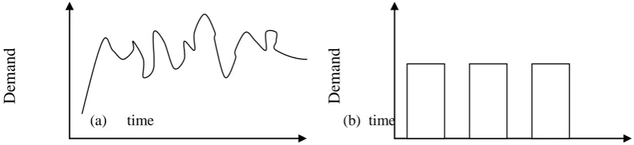
Therefore, the conclusion is drawn that the estimate of demand for a particular asset is a key factor in the policy of inventory determination and order formation. There are basically two demand models (Figure 1):

1. Independent (demand for one type of inventory does not depend on demand for another type of inventory) and

2. Dependent demand model (demand for one type of inventory depends on demand for another type of inventory).

Stocks in the independent demand system carry their name directly from the notion of independent demand, which implies a demand determined by the market, i.e. Demand formed outside the production process. In the first place, the price of products, consumer income and many other circumstances affect the demand. These are the most common stocks of finished products or stocks of spare parts designed to replace the defective parts of a product.

[image:3.595.65.522.367.472.2]

(a) time (b) time

Figure 1. Demand models: (a) -independent demand, (b) -dependent demand

Unlike independent demand, dependent demand depends on someone's demand for parts or components. Its importance is that production takes place in batches. An example of the car was adopted to explain these two demand. The very demand for cars is an independent size from the point of view of production management because it is determined by the market. However, demand for automobile wheels is dependent on size and is derived from demand for cars (it is done on the basis of the relationship that one car has four points). Therefore, demand for wheels depends on the demand for cars as the final product.

Different demand models are the basis for different approaches to inventory management. Independent demand is an inherent philosophy of complementarity, while dependent demand is oriented to the philosophy of need. The complementary philosophy means that supplies are immediately replenished after their reduction in order to ensure that goods are always ready for customers. In addition, the exit from the warehouse is also a signal for sending orders for additional quantities.

The philosophy of needs starts from the fact that the size of the orders should be based on the needs for a high level of material, which means that by reducing the stock, no additional quantity of raw materials is ordered. Additional quantities are ordered only if the request arises from the need for greater stock in the future.

The differences between dependent and independent demand have made significant progress in inventory management and production management. With independent demand for inventory management, various types of models have been developed that can be used to complement inventory, the most well-known model of an economical amount of orders. On the other hand, different demand models have been developed with the demand for inventory, the most important being the Material Requirements Planning (MRP) and the Manufacturing Resource Planning (MRP II).

In the continuation of the paper, these models are described in more detail, which are used both for the management of the stock of one chain participant as well as at the level of the entire logistics network. It is necessary to identify the most important factors that influence the policy of the stock. The most important factors are:

De

(4)

International Journal of Emerging Technology and Advanced Engineering

533

1. The first and most important is the demand, it can be known in advance or unreliable. In this latter case, foresight forecasting techniques (based, inter alia, on data on past demand) can be applied. Based on them, the voltages of different sizes of future demand can be estimated.

2. the time of replenishment of the stock. This time may be known at the time the order is sent or may contain a dose of unreliability.

3. number of different products stored in the warehouse.

4. The length of the period for which inventory policy is set.

5. costs, which include ordering costs and storage costs.

I. The cost of an order usually consists of the price of the product and the purchase.

II. the costs of storing the stock include: a. taxes and insurance.

b. maintenance costs.

c. loss of value of goods due to the market situation.

d. interest on assets invested in goods.

6. Require the level of service to the buyer. In cases of insecure demand, it is often impossible to ensure a 100% availability of goods, and an acceptable level of availability is required.

III. MODEL OF ECONOMICAL ORDER QUANTITIES Here are some of the inventory management models from Simchi-Levi's D .; Kaminsky, P .; Simchi-Levi, E.

The model of economical order quantities is a simple classical model that shows the relationship between purchase price (ordering) and warehousing.

There is a warehouse that has regular requests for delivery of only one product. The product is supplied by a manufacturer who is presumed to have unlimited capacity. The model includes the following assumptions:

1. The demand is constant and amounts to D pieces per day,

2. The order of the warehouse to the supplier is constant and amounts of Q products per order, 3. Fixed costs of realization of each order are K of

cash units,

4. The cost of storing the stock is h per day for one product,

5. Purchase time (the time has elapsed since ordering order to earlier commodities) is zero,

6. The initial inventory is zero, 7. Planning period is long (unlimited).

Optimal ordering is required, so that the total cost of the purchase order and the cost of storing the inventory are minimal and that there is no lack of merchandise at any time. This is an extremely simplified version of the real situation. However, the conclusions that arise from the analysis of this model help in the realization of an efficient stock policy of complex, realistic problems. Since the order is currently being implemented, it is easy to see that the optimal inventory policy for this model assumes a new order order, only when the inventory falls to zero. This reduces storage costs. In order to find the optimal order, consider the stock level in the time function (Figure 2).

Figure 2. The ratio of stock and time

Since the stock level changes from Q at the beginning of the cycle to 0 at its end, and the demand is constant and is D per unit of time, then:

Q = T  D

A simple account gives an optimal order size that is the smallest amount of these costs. By searching for extrusion of the cost function by quantity of purchase Q, an economic quantity of order is obtained:

S

uppli

es

Average level Stock Size

(5)

International Journal of Emerging Technology and Advanced Engineering

534

2

0

2

*2

h

Q

D

K

Q

h

Q

D

K

dQ

d



























h

D

K

Q

*



2 



This simple model points to two conclusions:

1. The optimal policy balances the ratio of the cost of keeping the stock and the fixed costs of order realization. The fixed costs reduced to the unit of time K * D / Q and the cost of keeping goods per day h * Q / 2.

With an increase in orders, the daily storage costs of h * Q / 2 are linearly increased, and the cost of the order divided by the time cycle K * D / Q declines. The economic size of the order is at the point where the lines of these costs are cut. This means that:

2 Q

h

Q

D

K



_



,

h

D

K

Q

*



2 



The average total cost per day, and therefore the total annual costs, are relatively insensitive to the size of the order Q.

In order to prove this claim, an order in the amount Q = b * Q *, where Q * is an economic order. For b = 1.2 order is 20% higher than economical.

2 Q

h

Q

D

K









* 2 * 2 * 2 2

2

2 b

Q

h

D

K

b

h

D

K

Q

b

Q

b

h

D

K

Q

h

D

K

Q

h

Q

D

K































b

Q

D

K

Q

b

D

K

b

D

K

Q

b

h

D

K

b

h

D

K

2 * * 2 * 2

1

2

2 _































For b = 1, the purchase quantity is Q = Q * and it is:

2

1

* 2 *









Q

D

K

b

Q

D

K

Then it follows that the ratio of total cost to the order Q = b  Q* ; (b  1), according to the cost of an economic order is equal:

b





2

1

2 .

The table 1. shows the influence of some values of variable b on the annual cost of the system.

(6)

International Journal of Emerging Technology and Advanced Engineering

535

Table 1.

The influence of the variable b on the annual cost of the system

b 0.5 0.8 0.9 1 1.1 1.2 1.5 2

Increase in cost

% 25 2.5 0.5 0 0.4 1.6 8 25

Table 1 shows that an increase in orders by 20% (b = 1.2) results in a cost increase of only 1.6%.

Planning of production and supplies in view of the unpredictability of demand

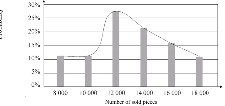
The previous model has shown the relationship between procurement costs and the cost of inventory of goods. The question of the unpredictability of demand was neglected. Many businesses plan production by relying on predicted demand, although they are aware of the possibility of wrong estimates. Due to newly emerging market conditions, demand estimate becomes more problematic, and the decision on production capacity is required based on a more detailed analysis of the likelihood of possible demand scenarios and the ratio of profits and costs that follow for a single production volume. For example, an enterprise that produces seasonal-type products is adopted, subject to frequent design changes. In order to organize production, approximately six months before the start of the sale, the company must plan production quantities for each of its products. Since there is no clear indication that the market will react to a new design, it is impossible to accurately predict the scope of future demand. By estimating higher demand, stocks will remain in the warehouses, while underestimated demand will lead to a shortage of goods and the loss of potential buyers and profits. The problem is accessed in such a way that the marketing sector is asked to make a predictable demand forecast based on sales data in past seasons, assessments of current market conditions and other relevant impacts and statistical methods. The likelihood of the size of the demand in any other case does not have to be assessed on the basis of a marketing estimate, but on the basis of some other relevant information.

This is usually the average demand and its standard deviation in previous periods. Based on such an assessment, it may be possible to obtain information that, for example, There is 11% probability that the demand will be 8,000 pieces, or 22% for 14,000 pieces. The prognosis can be requested for a certain range of quantities and shown graphically (Figure 3.3).

The question arises as to how to use this data for planning production volumes? In order to answer the question asked, the following information should be introduced for consideration:

a. What are the fixed costs of production (production start-up costs)?

b. What is the unit cost of production? c. What is the selling price of the product?

d. What is the discounted price of the product, if it is not sold within the due time?

All these data are needed to find the answer to the final question that reads: What is the volume of production for which the highest profit will be generated? To get the answer to this question, we will mention the following example. The following assumptions are set:

1. The costs of starting the production amount to 100,000 monetary units (NJ).

2. The cost of production of one product is 80 NJ. 3. The selling price of the product is 125 NJ.

4. The discounted price of the product not sold in the season is 20 NJ.

(7)

International Journal of Emerging Technology and Advanced Engineering

536

.

[image:7.595.82.472.140.324.2]

Number of sold pieces Figure 3. Potential demand

The following assumptions were adopted:

1. a decision was made on the production of 10 000 products,

2. total demand will be 12 000 products.

The realized profit can be easily calculated as sales revenue, minus the fixed, minus the variable production costs:

Profit = 125  10 000 – 100 000 - 80  10 000 = 350 000

In the event that 8000 products are sold for the same production in the final sales balance,and 2000 at the discount price, the profit is:

Profit = 125  8 000 +20  2 000 – 100 000 - 80  10 000 = 140 000

From Figure 3. it is noted that the probability of demand for 8000 pieces is 11%, and for 12 000 pieces 27%. This means that for production of 10 000 pieces with 27 percent probability, a profit of 350,000 NJ will be foreseen, and a profit of 140,000 NJ with 11% probability. Similarly, for the production of 10,000 pieces, the profit and probability of each possible sales scenario can be calculated. It is concluded that it is possible to find an average profit related to the production of 10 000 pieces of products, which derives from a collection of profits for all variants of placements in relation to the likelihood of their occurrence.

Clearly, the goal is to find the volume of production that gives the highest average expected profit. This production quantity is considered to be optimal.

The question arises, what is the relationship between the optimal production batch and the average estimated demand (in the case of 13 000 products), or is the optimal production equal, greater or less than the average predicted demand? In order to answer this question, the term marginal profit is introduced, that is, the marginal loss on the production of an additional product. For this case, if the produced additional product (thirteen thousand and the first one) succeeds in selling at the appropriate time, an additional profit equal to the proceeds from the sale of this product will be realized, minus the cost of its production, which for the given case is 45 NJ. If the product is not sold in time, but at a discount price, then it will yield a negative income or loss that will amount to 60 NJ for this case.

It follows that for this case, the loss due to the unsuccessful sale of the additional product is greater than the possible profit that would result in its sale. It is concluded that the optimal production volume is lower than the average predicted demand. In Figure 3.5. Is shown the average profit in the function of the production quantity, for this case (it is assumed that the monetary units are US $).

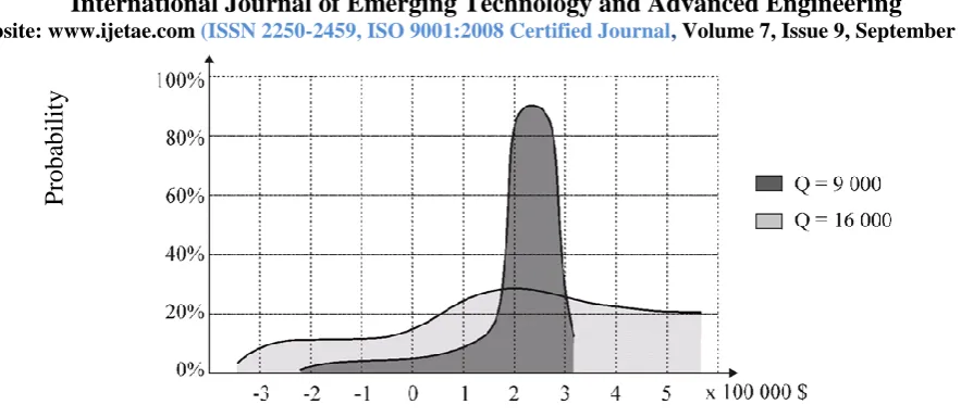
Logically, the question arises: if, for some reason, it is necessary to select production in the size of one of these series, which one to choose? To answer this question, it is necessary to study the risk associated with a particular decision. For this purpose, it is possible to construct a presentation of the relationship between the achievable profit and the probability of its occurrence for each of the production variants. Figure 4 Gives a principled view of this case.

P

roba

bil

it

(8)

International Journal of Emerging Technology and Advanced Engineering

[image:8.595.74.516.110.302.2]

537

Figure 4. Probability of profit

The need for constant stock

The value of knowing the anticipated demand in the previous case, which implied that the decision on the procurement of goods, or planning production capacity, is made only once in one business period. In most cases, these activities can be divided into several phases during this period (year). Unlike the ideal case in the analysis of the optimal order model, in a real situation, every participant in the distribution chain has the need to have certain supplies of goods at all times. The reasons for this are easily understood, and can be explained on the example of the distributor. He is forwarding his orders to the manufacturer. The manufacturer can not currently meet the set requirements (as presumed by the ideal model), but there is a certain amount of time for the implementation of each order. In addition, the distributor's estimate of the demand is not absolutely safe, it already contains some unreliability. From this it can be concluded that there are at least three reasons why the supplier must provide supplies during the period of order realization:

 To meet the forecast demand in the period when the ordered goods have not yet arrived from the manufacturer.

 Cover the uncertainty of demand assessment.

 Due to the optimal ratio of the cost of owning the inventory and the fixed costs of the realization of the new order.

The same situation is repeated by moving at different levels in the distribution chain. Thus, the manufacturer must provide his supplies of parts for installation and materials, his suppliers, etc. The reasons for keeping the stock are pretty clear. However, what is the optimal strategy for inventory management, that is, the planning of production capacity? The answer to this question includes two cases.

The first is when there are no fixed costs, which do not depend on a new order or production, but the total cost is equal to the product of the unit price and the required quantity of goods. The second case involves fixed costs, which are the same for any requirement that does not depend on its size. Here, the total cost is equal to the sum of the fixed costs and products of the unit price and quantity.

Case without fixed costs

It is assumed that:

1. The daily requirement is random variable, and follows the rule of normal distribution. Such demand is described by mean value and standard deviation.

2. No fixed order costs.

3. The storage price is expressed in cash per unit of product and time.

4. The company accurately indicates the level of product availability. It is likely that it will not be in the situation that it is currently left without goods. In order to describe the required inventory management model, the following data is required: AVG = Average value of daily demand

STD = Standard deviation of daily demand

L = The time of delivery of the goods, ie the realization of the order (from the supplier)

h = Unit price per unit of time (per day)

 = Degree of availability (means that the 1-).

Because the time of purchasing goods is not currently available, the total amount of products on their own warehouse and the products ordered and not yet received is called the "stock position".

The economical order quantity for the ideal case was equal to the equation:

P

roba

bil

it

(9)

International Journal of Emerging Technology and Advanced Engineering

538 h

AVG

K

Q

*



2 



h

AVG

K

h

D

K

Q

*



2 





2 



Since the fixed cost of realizing order K equals zero, it follows that Q * = 0.

For the considered case, there is no need to optimize the order with regard to the fixed costs, so the theoretical optimum inventory policy is, according to the "min-max" model, when s = S. In other words, whenever the stock position falls below the optimum level s = S, New order to this same level. This practically means that the goods should be ordered after each sale. Ideally, the order time was zero, and demand was well known. Our case assumes the time of order execution L, and the uncertainty of the estimation of demand. Because of this, the position of the stock to be ordered is not zero, as in the ideal case. This stock position with has two components. The first component represents stocks that cover the average demand expected during the acquisition period. It is equal to the average daily demand product and the time it takes to complete the order:

L  AVG

The second component represents a security stock. This is the amount of stock that is required to withstand the appropriate degree of probability to cover the deviation of the average demand at the same time L. The amount is given by the following expression:

L

STD

z



_,

Where z is the constant which requires a certain with, for the sake of the above and the S position, to which the stocks are supplemented:

S

L

STD

z

AVG

L

s











Case with included fixed costs

In this case, whenever the inventory is supplemented, additional costs for K are paid, which do not depend on the size of the series (eg, the cost of production preparation, freight cost, ...). (S, S) the model of stock supplementation can not be set by the same principle. The point from which the stores are renewed with and the level of renewal of S are different then. In analyzing the example of single-season production, it was concluded that this difference is a consequence of fixed costs of ordering or production. Here the stock status, indicative of the new order, is as in the previous case:

L

STD

z

AVG

L

s









The first component covers the average demand for the realization of the next order (time L), and the other with the given security covers demand deviation at the same time. The level complemented by S stock, the following logic is set up when analyzing the Harrison model. There is an optimal size of the order, depending on the fixed costs:

h

AVG

K

h

D

K

Q

*



2 





2 



When there is no deviation in demand, the quantity of Q = Q * should be ordered, each time the total level of complete the order. However, demand is volatile, so uncertainty should be covered by an additional amount, in the amount:

z



STD



L

, where the factor z applies as well as the required availability of the goods. Stock position S depends on fixed costs K:

If K = 0 , Q  0 we come to the previous case without fixed costs:

s

L

STD

z

AVG

L

S











With the growth in Fixed Costs K, Growth and Equipment also grow:

It should be noted that the ideal case assumed the current execution of the order, or L = 0.

In the real case, the procurement time L is different from zero. If the fixed costs are so small that Q * <L * AVG is valid, this means that the Q * order can not cover the average demand at the time of procurement, which is equal to L * AVG.

Veličina fiksnih troškova K , za koje ovo važi, proizlazi iz:

2

*

2 AVG

L

h

AVG

K

Q









2 2

2 AVG

L

h

AVG

K



_

_





2

h

L

K





In this case (Q < L  AVG) level S is further calculated as:

s

L

STD

z

AVG

L

S











_.

For

2

h

L

K





(10)

International Journal of Emerging Technology and Advanced Engineering

539

In this case, the fixed costs are so high that it is not payable to order the new goods continuously, so:

s

L

STD

z

Q

S









_.

In general it can be said that the level at which stocks are filled is the same:



Q

L

AVG



z

STD

L

S



max

,







_,

Where

max



Q

,

L



AVG



this means greater value than Q ili L  AVG .

Uncertin time of income

In many cases, the assumption about the known time that will pass from placing the order to its implementation is unreliable. Thus, the uncertainty of this time, assuming its average AVGL value and the standard deviation of STDL, should often be considered. In this case, the point s, to which the request for supplementary stock is referred is:

2 2

2

STDL

AVG

STD

AVGL

z

AVG

AVGL

s













Where AVGL  AVG represents the average demand at the time of procurement, and

2 2

2

STDL

AVG

STD

AVGL







_standard

deviation of demand over that time.

So the security stock is the same:

2 2

2

STDL

AVG

STD

AVGL

z







The level to which the stocks are supplemented is equal to the sum of the security stock and greater than the quantity Q and the average demand in the middle of the order realization:

Z is selected from the table 3.2. II. CONCLUSION

The best inventory is managed on a number of models. The most efficient stock management model was introduced at the beginning of the last century. Today there are no such models. This research is divided into traditional and modern stock management. Purchase Cost (EOQ) is based on traditional models. Modern models have been developed: Just Time (JIT), Material Requirements Planning (MRP) and Deployment and Market-driven Funds (DRP).

Particular attention is paid to Modeling and Controlling Inventory Design (DRP) based modeling and control as it is the smallest model in local scientific and professional literature. Market Distribution Planning and Control (DRP) is a plan for timely inventory planning at all levels of the distribution network. DRP models enable warehouse management across the entire mills, distribution centers, and hundreds of markets in the distribution network. This is their biggest advantage in MRP models that are applied separately to each plant. DRP designs provide an efficient production plan and development of a traffic plan as well as traffic co-ordination with a supplier. DRP models are delivered via a distribution system. Inventory was started at the end of the distribution network at retail level. The funds required from stock (retail) are generated after the adjustment to remove the bookkeeping and the negative effects of the size.

Today, big companies have a good inventory management strategy, so there are a number of templates that you can design and produce. In fact, every member of a distribution chain must normally have a feature or safety component at any time, so it is virtually impossible to set zero in the inventory. Nowadays large companies pay close attention to measuring the logistics chain's performance and logistics processes, so we can not speak of a unique stock model, but some models are partially or individually inventory. Used in conjunction with all interconnected and complementary means and controlled by each Member State Reduces the minimum number of shares; E. reducing costs. The global supply chain has many other problems. This is because the supply chain is huge, the management time is far too long and there are many things like currencies, policies and laws. It produces different currencies and forecasts in different countries, different tax laws, different trade protocols, as well as transparency and profitability.

REFERENCES

[1] Ammer, C.; Ammer, D.S.: Dictionary of Business and Economics, The Free Press, London, 1984.

[2] Bertolini M & Rizzi A. A simulation approach to manage finished goods inventory replenishment economically in a mixed push / pull environment. Volume 15.Number 4.2002:1-2.

[3] Biggart T B & Gargeya V B. Impact of JIT on inventory to sales ratios. Volume 102. Number 2002:1

[4] Blanchard David (2010), Supply Chain Management Best Practices, 2nd. Edition, John Wiley & Sons

[5] Bloomberg D J, Lemay S & Hanna J B.2002. Logistics. Prentice Hall. New Jersey.USA

[6] Bowersox D J, Closs D J & Cooper M B.2002. Supply chain- Logistics management. International Edition. M C Graw Hill. USA.

(11)

International Journal of Emerging Technology and Advanced Engineering

540

[8] Chandra C & Kumar S. Taxonomy of inventory policies for supply-chain effectiveness. Volume 29. Number 4. 2001:3.University of Pretoria

[9] Coyle, J., Bardi, E., Langley, J., The Management of Business Logistics, sixth edition, West Publishing Company, St. Paul, 1996 [10] Feller Andrew, Dan Shunk, & Tom Callarman (2006). BPTrends,

March 2006 - Value Chains Vs. Supply Chains

[11] Flores, B. E.; Whybark, D. C. Multiple criteria ABC analysis. International Journal of Operations and Production

Management. 6, 3(1986)

[12] Gourdin K N. 2001. Global logistics management. A competitive advantage for the new millennium. Blackwell Business. USA [13] Heizer, J. & Render, B. (2004): Operations Management, seventh

edition, Prentice Hall.

[14] Hines, T. 2004. Supply chain strategies: Customer driven and customer focused. Oxford: Elsevier

[15] Hugo W.M J, Badenhorst-Weiss J A & van Rooyen D C. 2002. Purchasing and supply management. 4th edition. Pretoria: J.L Van Schaik Publishers.

[16] Jacoby David (2009), Guide to Supply Chain Management: How Getting it Right Boosts Corporate Performance (The Economist Books), Bloomberg Press

[17] Krajewski L J & Ritzman L P. 1999. Operations management. Strategy and analysis. 5th edition. Addison-Wesley. USA. [18] Lambert, Douglas M.Supply Chain Management: Processes,

Partnerships, Performance, 3rd edition, 2008.

[19] Mentzer, John T., William DeWitt, James S. Keebler, Soonhoong Min, Nancy W. Nix, Carlo D. Smith, & Zach G. Zacharia (2001): Defining Supply Chain Management. Journal of Business Logistics, Vol. 22, No. 2

[20] Monczka R, Trent R & Handfield R., Purchasing and supply chain management.. South-Western / Thomson Learning. USA, 2 edition 2002.

[21] Ng, W. L. A simple classifier for multiple criteria ABC analysis. // European Journal of Operational Research. 177(2007)

[22] Ramanathan, R. ABC inventory classification with multiple- criteria using weighted linear optimization. // Computers and Operations Research. 33(2006)

[23] Rushton Alan; Croucher Phil; Baker Peter, The Handbook of Logistics and Distribution Management, Kogan Page, London, 2010

[24] Partovi, F. Y.; Burton, J. Using the analytic hierarchy process for ABC analysis. // International Journal of Production and Operations Management. 13, 9 (1993)

[25] Schonsleben P. 2000. Integral logistics management. Planning & Control of comprehensive. Business processes. The St-Lucie Press / APICS Series.

[26] Simchi-levi, D.; Kaminsky, P.; Simchi-levi, E.: Designing and Managing the Supply Chain, Mc Graw-Hill Higher Education, Boston, 2000

[27] Smaros J et al. The impact of increasing demand visibility on production and inventory control efficiency. Volume 33. Number 4. 2003:1

[28] Raman, A., DeHoratius, N., Ton, Z. (2001): Execution: The Missing Link in Retail Operations, California Management Review, 43 (3)

[29] Rusli Khairul Anuar, Azmawani Abd Rahman and Ho, J.A. Green Supply Chain Management in Developing Countries: A Study of Factors and Practices in Malaysia. Paper presented at the 11th International Annual Symposium on Sustainability Science and Management (UMTAS) 2012, Kuala Terengganu, 9–11 July 2012.

[30] Supply chain management (SCM). APICS Dictionary. Retrieved 19 June 2014

[31] Schroeder, R.G:: Upravljanje proizvodnjom, Mate, Zagreb, 1999. [32] Vollman, T.; Berry, W.; Whybark, M.: Manufacturing Planning

and Control System, Irvin, Boston, 1992.

[33] Wieland Andreas, Carl Marcus Wallenburg (2011):

Supply-Chain-Management in stürmischen Zeiten. Berlin.

[34] Wiendahl, H.-P.: Load-Oriented Manufacturing Control, Springer Verlag, Berlin, Heidelberg, New York, 1995.

[35] Wight, O.: Manufacturing Resource Planning, MRP II, Essex Junction, Oliver Wight LTD. 1984.