Revisiting variance gamma pricing : an application to S&P500 index options

Revisiting variance gamma pricing : an 

application to S&P500 index options

Mozumder, S and Sorwar, G

http://dx.doi.org/10.1142/s242478631550022x

Title Revisiting variance gamma pricing : an application to S&P500 index  options

Authors Mozumder, S and Sorwar, G

Type Article

URL This version is available at: http://usir.salford.ac.uk/34856/ Published Date 2015

USIR is a digital collection of the research output of the University of Salford. Where copyright  permits, full text material held in the repository is made freely available online and can be read,  downloaded and copied for non­commercial private study or research purposes. Please check the  manuscript for any further copyright restrictions.

Revisiting Variance Gamma Pricing: An Application to S&P500 Index Options

Sharif Mozumder1 Ghulam Sorwar2

Kevin Dowd3

May 18, 2015

1_{Corresponding author; Associate Professor of Mathematics, Department of Mathematics, University of} Dhaka, Dhaka, Bangladesh. Email: [email protected].

2 _{Professor of Finance, Salford Business School, Lady Hale Building, Salford M5 4WT, United Kingdom.} Email: [email protected]. Corresponding author.

Revisiting Variance Gamma Pricing: An Application to S&P500 Index Options

Abstract

We reformulate the Lévy-Kintchine formula to make it suitable for modelling the

stochastic time-changing effects of Lévy processes. Using Variance-Gamma (VG)

process as an example, it illustrates the dynamic properties of a Lévy process and revisits

the earlier work of Geman (2002). It also shows how the model can be calibrated to price

options under a Lévy VG process, and calibrates the model on recent S&P500 index

options data. It then compares the pricing performance of Fast Fourier Transform (FFT)

and Fractional Fourier Transform (FRFT) approaches to model calibration and

investigates the trade-off between calibration performance and required calculation time.

1. Introduction

In the seminal papers by Black and Scholes (BS) (1973) and Merton (1973) the

underlying distribution driving the option price is the lognormal distribution, which itself

reflects the underlying assumption that returns follow a Geometric Brownian Motion

(GBM). However, the use of GBM as the benchmark process for describing asset returns

in continuous time does not allow for some key features of stylized asset price behavior:

in particular, it fails to allow for (i) asset price jumps, (ii) conditional skewness in returns,

(iii) conditional excess kurtosis in returns, (iv) stochastic volatility or (v) any correlation

between returns and their volatilities. These well-established features of empirical return

process have encouraged researchers to develop alternative models in which GBM has

been replaced with more sophisticated processes, including GARCH processes, stochastic

volatility processes and Lévy processes, which are the focus of the present paper.

Lévy processes can deal with each of these deficiencies, and therefore have considerable

potential for option pricing: (i) Traditionally, jumps in asset prices have been modeled by

the compound Poisson process which allows for a finite number of jumps within a finite

interval. However, we often observe that asset prices display many small jumps on a fine

time scale, and this suggests that Lévy processes which allow infinite numbers of jumps

to occur within a finite time scale may be more suitable for modeling jumps. (ii/iii) Lévy

processes can easily accommodate both skewness and excess kurtosis in returns. (iv)

Lévy processes can accommodate stochastic volatility by applying stochastic time change:

this is the equivalent to stochastically altering the clocks on which the Lévy process is run.

time, a more active business day implies a faster clock. (v) To model the correlation

between returns and their volatilities, we let the innovations in the Lévy process be

correlated with the innovations in the random clock on which it is run. When this

correlation is negative, the clock tends to run faster when the Lévy process falls (Carr and

Wu (2002)). In summary, time-changed Lévy processes parsimoniously capture all five

main deficiencies of Brownian motion. Furthermore, Lévy processes lead to analytically

tractable models which simplifies parameter estimation and model calibration.

In this study we seek to make a number of contributions to the Lévy option pricing

literature. First, we reformulate the Lévy-Kintchine formula on which Lévy processes are

based: this allows us to explicitly clarify how additional shocks to the Brownian motion

dynamics can be regarded as the superpositions of compound Poisson and compensated

compound Poisson paths. Our reformulation is helpful for modeling the time-changing

effects, aids in both the simulation and parameter estimation of Lévy processes, and has

ready applications to Lévy option pricing. Second, we use this reformulation to visit the

earlier work of Geman (2002): we are able to demonstrate a misspecification in this work

and provide a correct solution to it. Third, using observed option prices based on the

S&P500, we calibrate the BS model and its time-changed Lévy version, the Variance

Gamma (VG) model. Fourth, we use two different Fourier techniques to value the options

and contrast their performance with each other. The two Fourier techniques considered

are the Fast Fourier Transform (FFT) and Fractional Fast Fourier Transform (FRFT)

suggested by Chourdakis (2005). In particular, we examine the trade-off between

This paper is organized as follows. Section 2 sets out the Lévy framework and provides a

reformulated version of the Lévy-Kintchine formula. Section 3 shows how this

reformulation can be used to derive the parameters of the VG model; this section also

revisits the earlier work of Geman (2002). Section 4 sets out the risk neutral specification

for the VG model which is used for pricing purposes. Section 5 outlines the FFT and

FRFT approaches to option valuation, and section 6 sets out and discusses the empirical

calibrations of the BS and VG model under FFT and FRFT, based on a weekly data set

for 2007. Section 7 concludes.

2. The Lévy Framework and Asset Pricing

We begin with the definition of a Lévy process and the Lévy-Kintchine formula for

infinitely divisible distributions.

Definition 2.1A cadlag stochastic process X={Xt;t≥0}, on (Ω,F,P) with values in  is called a Lévy process if it satisfies the following properties:

[L1] each X₀0 . .a s

[L2] Xt has independent and stationary increments, i.e.

(i) for every increasing sequence of times t₀ t₁t₂ ...t_n the random variables

1 0

1

0, t  t ,..., tn  tn

t X X X X

X does not depend on t.

(ii) _{t h t h},

D

t h

t X X X

X _   _{ }  i.e. the distribution of X_th X_tdoes not depend

on t.





, 0 lim

0     

 t h t  

h P X X

Condition [L3] implies that for a given (deterministic) time t the probability of having a

jump at t is zero, i.e. discontinuities (jumps) do not occur at deterministic times and so

must occur at random times.

2.1. The Lévy-Kintchine Formula

We now use the Lévy-Kintchine formula to derive distributional characteristics of a Lévy

process.

Theorem 2.1 FM₁

 

 is infinitely divisible if there exist scalars a,b and a

measure ν satisfying 

 

 

0 0and



_{ }



x 





 

dx 

0 \

2

1 such that for alls:



 

 _  





  _{ }

 



 

_

 e isx  x dx b

s ias

s is x

F 1,1 

2 2

1 2

1

exp (1)

Conversely any mapping of the above form is the characteristic function of an infinitely

divisible probability measure on . Thus the parameters "a", "b" and the measure “ν”

characterize the distribution of the underlying infinitely divisible random variable and

(a,b²,ν) is known as the characteristic triplet or Lévy triplet of the underlying infinitely

divisible random variable.

The derivation of equation (1) can be found in Sato (1999), Applebaum (2004) or Cont

and Tankov (2004). The last term in (1) can be written as:





 





 

  

 _

  



_

_{ }

_



 e isx dx x e dx

is x

x

is x  

1

1 1 exp 1

Following Applebaum (2004), we set



 

A 



F

 

A and equation (1) becomes:





 





 

  

 _

  



_

_{ }

_



 e isxF dx x e F dx isx

bj x

isx sj

1

1 1 exp 1

exp   (3)

where “sj” and “bj” stand for small jumps and big jumps respectively.

The last part of equation (3) is the characteristic function of “big” random jump sizes

|x|>1, controlled by a compound Poisson distribution with intensity:



 



 1 x

bj  F dx

 (4)

and the jump distribution:

 

 

 

 



  



 

 

1 1 1

1

x x

bj x J

dx F dx dx

dx F

  



(5)

where _bj_sj and the random variable, J describing the jumps of all sizes (with

intensity of jumps of all sizes 

 

 F

 

 ) has distribution F(x). Thus:







1







_{ }

1





1

1

1 

 





 

x J

dx F x x

F

 

Consequently, the last part in equation (3) is the characteristic function of the Compound

Poisson process CP



bj,F_J1

 

dx



.

For its part, the first part in equation (3) is intuitive and can be seen as a limit

corresponding to



_i0 as i , viz.:

exp _sji _eisx₁_isx _ix1







F dx

 

i



 

 



1 1



exp i Fi J isJ 1 i Fi J

sj sj

i

E  e is E  J

 

     

 _{ } 

 _{ }  _{ }





 (6)

(since J is F-distributed)

exp



_sji



_eisx ₁_isx_Fix1

 

_dx



i



     

exp _sjeisx 1isxF dx

 

x1



 



 as i  (7)

where  1  2 .... i ....

s j s j s j s j    _{ } 

 is the overall intensity of small jumps. The limit in

equation (7) is the characteristic function of a compensated (mean subtracted) square

integrable random variable (see Kyprianou (2006)). For a general n each n

sj



 and

 

dx F _J

n 1

 are given respectively by:



  1



 n n

sj x

n   

 (8)

 

        _      _n n n n n sj x x dx

F_{ } _ 

  1 1 1 (9)

The overall intensity of small jumps with magnitude less than one is then:

_sj  





₁< x 1



U



₂< x 1



U...U



_n<x 1



U...





1



n x    

 

1

x F dx









(10)

Now consider an arbitrary summand in equation (6):















E e

 

is E J



The first part in (11) corresponds to the characteristic function of a random variable

 



F dx



CP

J _J s j _J

N

j j i

i j

i 1 1

1   ~ ,  

 







  with sjn



 and _J1

i

F_ given by equation (8) and

equation (9) respectively (see Cont and Tankov (2000))). Here

 

i

sj

Poisson

N ~



 and hence we obtain



J



E

 

N E J E J

E N _J F _{s j} F J

j j i i J i j i 1 1 1

1  

       



  

  , implying that the second part in

equation (11) is the characteristic function of a constant equal to the mean of

 



F dx



CP _{sj J} i i

1

, _{  }



 . Hence equation (11) is the characteristic function of a compensated

(mean subtracted) compound Poisson random variable of small jumps (sj), which we

denote as J E J CP



F

 

dx



j i i i

j

i s j J

c J

F

J N

j j 1

1

1

1 ~ ,  

      



    

. Since this is true for each

summand, equation (6) is the characteristic function of the sum of a possibly infinite

number of compensated compound Poisson random variables:



, ₁

 





, ₁

 



...



, ₁

 



...

2 2 1

1    

  

 

 dx CP F dx CP F dx

F

CPc _{s j J} c _{s j J} c _{s j J}

i i       _{ }

 (12)

The compensation is required to obtain the convergence, as in equation (7), of numerous

small jumps described by possibly infinite number of compensated compound Poisson

random variables, to a compensated square integrable random variable whose

characteristic function is exactly the first part of equation (3).

Thus equation (1) characterizes the limiting distribution of the sum

of 

 





_

 







_i





s j _J

 





c

J

bj F dx CP F dx

CP b

N

a 2 _{1 1}

1 1_,

, ,

0   _ where the rates and

distributions of big and small jumps are as described above.

We now replace the noise process in the standard Black-Scholes dynamics with an

arbitrary Lévy process Xt:

_t

t

t _{dt dX}

S dS



ˆ (13)

where the usual volatility σ is set to 1 for simplicity. Integrating on [t1,t2], we obtain an

infinitely divisible random variable describing the random evolution of log returns on

[t1,t2]:









_{ } 2 2 1 1 2 1 2 1 2 1 ˆ ln ˆ t t t t D t t S

t t X X

S

t t X

  _                (14)

by [L2](ii) in Definition 2.1. According to the Lévy-Kintchine formula the distribution of

1 2 t

t X

X  is characterized by the characteristic function of an infinitely divisible random

variable given by:



 









_{ }

 



 

  _     _{   }     _  

_

   0

\ 1,1

2 2 1 2 1 2 1 exp 1

2 _{t t ias s b e isx x dx}

e

E is Xt t is x 

(15)

Thus following section 2.1, we can rewrite (14) as:

   





       





 





       





2 1 2

2 1 2 1 2 1 2 1 1

2 1 1

0

2

2 1 2 1 2 1 1

2 1 1

0

ˆ

ln N 0, ,

,

ˆ N 0, ,

,

lim

lim

i i i i i i D t bj J t c sj J i i D bj J c sj J i i S

t t a t t t t b CP t t F dx

S

CP t t F dx

t t t t b CP t t F dx

CP t t F dx

where ˆa . The rates _bj and i

sj



 as well as the distributions F_J1

 

dx and

 

1

i J

F_{  } dx of big and small jumps, respectively, are as described in section 2.1.

2.3. Changing Time through Subordinator Processes

Subordinators are stochastic processes which are used to introduce randomness in the

time axis. An intuitive interpretation of the purpose of such stochastic processes,

replacing calendar spacing of time with ‘business’ spacing of time, is discussed in Geman

(2002). The occurrence of events is then modeled using business time instead of calendar

time.

Definition 2.2 (Subordinator) Let {Xt;t≥0} be a Lévy process such that Xt has the Lévy triplet (a,b²,ν). Then Xt is an increasing process in t if and only if







 

_

1

 

 0

2

, 0 , 0 0

, b x dx

 and 1

 

0

0 



a



x dx

d  . Such an increasing process

is known as a subordinator.

In this case Xt can be expressed as the sum of both its linear drift and its jumps over times

0 to t:

_{ }





, 0

1 0 ,

0     









  

 xJ ds dx dt X t dt

X

s

X t s

s

t X

t (17)

and its characteristic function is expressed as:

E

 

eis Xt _exp



t



ids





eis x₁





 

dx





(18)

where



 



 

1

x x dx

a

Thus in the case of the subordinator drift being positive and there being no negative

jumps in the time process, the diffusion component needs to be zero, since otherwise

there will be a positive probability of a negative change in time over any interval.

Consequently, positive jumps are the only source of randomness and finite variation

ensures that small jumps are summable. This implies that the usual compensation of

small jumps in the Lévy-Kintchine formula (to ensure the integrability of the Lévy

measure) is not needed and the compensation part can be adjusted with the drift of the

process to give a new drift. (Further details can be found in Cont and Tankov (2004) and

Sato (199)).)

The following theorem shows that when a Lévy process modeling return dynamics is

subordinated by a subordinator (modeling time change) then the resultant process is still a

Lévy process. Moreover it shows how to obtain the characteristics of the resultant process.

Theorem 2.3 Let Tt be a subordinator with Lévy measure ~, drift d. Its distribution at time t,

t

T

P is characterized by the equation (18) and let

1

T

P



 . Further assume that Xt

is a -valued Lévy process with Lévy triplet (a,b²,ν). Its distribution t

X

P , at t>0 is

characterized by equation (1) and let

1

X

P



 . Then provided the processes Xt and Tt are

independent, the process defined as

 

 

 

0;

X t

Y_t  _Tt  (19)

is also a Lévy process. The distribution of Yt is given by:

The Lévy triplet



a_y,b_y2,_y



of Yt is given by:



 



 

 

 

1 0

~ .

x s

y da ds x dx

a   (21)

by2 d.b2 (22)

 

.

 

   

~ ,



\

 

0



0 



d B

_

 B ds B

B s

y   

 (23)

The proof of the above theorem can be found in Sato (1999). We now explore VG

process using theorem 2.3 to relate its dynamics to equation (16).

3. Revisiting Variance-Gamma as a Time-Changed Process

The Variance Gamma (VG) process introduced by Madan et al. (1998) involves

time-changing Brownian motion by an increasing gamma process. Gamma random variables

are infinitely divisible and so, according to the Lévy-Kintchine formula, a gamma process

can be obtained such that:

_

       

       

 _{   }

1 , general

in 1

, T t

s T

T_{t s t t} (24)

where 



,



has the density:

   

1 ; 0, 0, 0



  _{ }



  

x e x x

f x (25)

(see Cont and Tankov, [2004]).

We now note the following two lemmas:

Lemma 3.1 The generating triplet for the 



,



distribution is (0,0,υs), where the Lévy

measure υs is given by:

 

 e dx,x0

x

dx x

s  

It then follows that the gamma process Tt in equation (24) with  1 and  1 is a

subordinator with triplet (0,0,tυs).

Lemma 3.2 If Kp is a modified Bessel function of third kind, then:

 

  

    

    



e t dt x p

x x

K t p

x t p

p ; 0,

2 2

1 1

0 4

2

(27)

 

_



_{  }



_

  

 

  

     







 

 

n

i

i x

n x

i i n

i n e

x x

K

1 2

1

2 ! !

! 1

2

2 1



(28)

The derivation of the above Lemma can be found in Watson [1944].

Now consider the process X_t B_tt, where Bt is a standard Brownian motion with

volatility and drift parameters  0 and >0. The VG process is then defined as

the process Y subordinated to X by the Γ-subordinator T:

Y_t X_T B_t T_t

t  



: (29)

The gamma process is characterized as in equation (24) so that it ensures the mean rate t

and variance γt with the probability density:

 

 

 

 





 t x t

t x x e

f

t T

 



 1 1

(30)

With this parameterization the Laplace transform of the gamma subordinator is:

_E

 

_esTt 



₁_s



t ₍₃₁₎

Equation (29) shows that, conditional on a jump of size Tt = s in the time change, the

characteristic function of the VG process is then obtained by conditioning on the subordinator, viz.:    

_{ }

 

_{ }





2 2 1 2 0 0 2 2 1 2 | 1

Tt t t

Tt t

t Tt t

t t

is B T

Y

is B T

t T

is u s u B T

T

E e

E e T u f u du

e f u du

s is 

                     _ _    _  _       _  _





(using equation (31))

2 2 1 2 1 1 t is s        _{ } 

  (32)

Applying Theorem 2.3 then yields the Lévy triplet of the VG process. From equation (21):

avg = [drift subordinator][drift subordinate]

 

₁

 

1

0 . 1

s B

dx yP_{ } dy





 







= 0.[drift subordinate]

 

 

1

1

1

0 . 1

x

s B

e dx yP dy x         

_

_

(using Lemma 3.1)

 

 2

2 2 1 1 0 1 1 . 2 y s x s

e dx y e dy

x s           



_

_

  (33)

From equation (22):

b_vg  [drift subordinator][drift subordinate] =0 (34)

also using Lemma 3.1.

From equation (23):

_vg [drift subordinator].[drift subordinate]+

   

1 0

s B

P_{ } dx



ds

 



 2 2 2 0 1 0 2 x s s s

e e ds

s s          _  

_

[with 1/ and  1/ using Lemma 3.1]

 2 3 2 2 2 0 1 2 2 x s s s

dx e s e ds

s            _{ }

Since   1 2 2 2 2 2 2 2 2 2 2     _                   s x x s s x _s s e e e

e  

     _ 

we now use (35) to obtain:

 



  









    _{ }       0 1 2 2 0 2 2 2 2 2 3 2 2 3 2 2 2 exp 2 2 ds s s dx e ds e s e dx s x s vg x s s x                 (36)

To evaluate the integral in equation (36) we need to use equation (27). We then set



_22







   and s



s and rearrange the integrand in equation (36) to obtain:

 

3 2 2 2 2 2 3 2 1 2 2 2 1 2 2 0 2 2 0 1 2 2 2 1 exp 4 exp 4 2 1 2 2 x x x s s ds s

s s ds

s x K               _        _{    }   _{  }   _{  }_           _ _{ }           _{ }   _{  }    _{   }     _{  } _





(37)

 

 

2 1 2 2 2 1 2 2 2 1 2 2 2 2 1 2 2 2 2 2 1 2 2 2 2 1 2 2 2 2 2 2 2 1 2 2 exp 2 1 2 exp x x vg x x x x K e dx e dx x x dx x x x dx x                         _            _{ }   _{ }   _{ }   _{ }       _{ }   _{ }   _{ }   _{ }       _  _      _   _

  (38)

The last equality follows by plugging back the value of κ with β = 1/γ.

The drifted Brownian motion, without time change, describes the assets log return

through two parameters μ and b as in equation (16) (without compound Poisson parts). As

equation (29) shows, the VG is a Brownian motion with a change of calendar time to

business time made by a gamma process. The parameters aνg and bνg play the same role

for the VG process as parameters a and b in equation (16) for a general Lévy process.

However, bνg being zero, equation (16) shows that the dynamics of the log returns have

no diffusion but only jumps. Furthermore ννg completely describes the rate and

distribution of both small and big jumps, as explained in section 2.1.

The derivation of the Lévy measure in the previous section helps us recognize that with

the specification of the parameters in Geman (2002), the form of the Lévy measure

mentioned therein is not correct (although her numerical work was not affected by this

error). We now derive the expression of Lévy measure as used by Geman and report the

correct specification of the parameters.

Geman et al. (2001) show that the VG process may be expressed as the difference of two

independent gamma processes:

tn p t

t G G

Y   (39)

where p t

G and n t

G are interpreted as the price changes from positive and negative shocks

respectively. Given equation (39), equations (31) and (32) then suffice to demonstrate

that:





2 2

1 2

2

1 1 1

1 1 1

1

1

p n

p n p n

is s is is

is s

    

   

   

_  _ 

  _  _{ }  _



  

(40)

which is equivalent to:

pn  (41)

2

2

 

_{p n}  (42)

Geman [2002] specified the solutions of (41) and (42) as:

2 2 4

2 2 2

1

    



  

p (43)

She went on to argue that with these specifications the Lévy measure of the VG process

can be written as:

 

         0 if 0 if x dx C x dx C dx x e x e g Gx Mx 

 (45)

where

p

n M

G

C_1_, _1 _, _1 _.

However using the derived form of Lévy measure (see equation (38)), one can see that

solutions (43) and (44) do not yield the expression of the Lévy measure (45). Moreover

(43) and (44) do not even satisfy (41) and (42).

To show the correct approach, we now solve equation (41) and (42) separately for ηp and

ηn. For ηp we write equation (41) as p n  . Then from equation (42) we obtain:





  2 2 4 4 8 4 2 2 2 2 2 2 2 2 2                           n n n

Then again from equation (42) we obtain:

2 2 2

2

1

2

4 2 2

p                    (46)





  2 2 4 4 8 4 2 2 2 2 2 2 2 2 2                           p p p

Then once again from (42) we obtain:

_n  1 2

2

22

4 

2

2   2       (47)

Our solutions satisfy equation (40). Moreover using equation (38), we now prove that our

solutions produce the form of Lévy measure mentioned by Geman.

From equation (38) for x>0 we obtain:

 

0 , 2 2 4 2 exp 1 2 1 exp 1 2 2 2 2 2 2 2                                           x x e C dx x x dx x x dx Mx g                _ (48) where p M

C_1_, _1 _{with ηp given by equation (46).}

Similarly from equation (38), since for x<0;∣x∣=-x i.e. x=-∣x∣, we obtain:

where

n G

C _1_, _1 _{with ηn given by equation (47). Equation (48) and (49) together}

imply (45). QED.

4. Risk-Neutral Specifications

To price the option we use the risk-neutral characteristic function. To obtain the latter, we

start with the characteristic function of the VG model under the real measure, given by

equation (32), rewritten as:

 

            _{ }        2 2 2 1 1 ln

exp t is s

s

t

Y (50)

We can extract two parts from equation (50): the drift part μ = 0 and the non-drift part

 



  



 _ 2 2

2 1

1

ln is s

s t   _{. The drift part under the risk-neutral measure can now be}

obtained (see Shiryaev, [1999]) as:

 

 

st i r st

t i r i s rn             _{ }       _         2 2 1 1 ln 1 (51)

The risk-neutral characteristic function can then be obtained as:

 



   



            _{ }              _{ }                2 2 2 2 1 1 ln 2 1 1 ln 1 exp exp s is t st r i s s

s r n

r n Y_t

(52)

Similarly, the real measure characteristic function of the Black-Scholes Brownian motion



t t



N

B_t ~  , is:

 

s



is t s t



t B 2 2 2 1

exp   



and its risk-neutral equivalent is

 

   



 _

   

   

rn_B s i r st s t

t

2 2 2

2 1 2

1

exp   (54)

Our empirical study is conducted under the risk-neutral measure utilizing the risk-neutral

characteristic functions (52) and (54).

5. Pricing with FFT and FRFT

Now consider s_t ln

 

S_t and kln

 

K where K is the strike price of the option. As in

Carr and Madan (1999), the value of a European call with maturity T is expressed as a

function of k:

C

 

k e



es ek



q_T

 

s ds

k r T

T 





 

(55)

where q s_T( ) is the risk-neutral density of the log of the prices. To overcome the non-square integrability of CT(k), Carr and Madan (1999) introduced modified call prices:

c

 

k e CT

 

k , 0

k

T (56)

where α is known as the dampening factor. Following Carr and Madan (1999) an analytic

expression for the pricing formula (55) can be obtained as:

C

 

k e e iuk _T

 

u du

k

T  





 





0 (57)

 





_





_

u i

u

i u

e

u T

rT

T

1 2

1

2

2   

  

 

 





 (58)

and where Ф is the characteristic function of the model for which prices are computed.

Using a suitable numerical integration technique, e.g. the trapezoidal rule, the integral

appearing in equation (57) can be approximated as:



 

_T

 

_j

N

j k iu T

iuk

u e

du u

e j ~

1

0

0







 

  _

(59)

where

T

~ _{is exactly as ψT with weights attached by the integration rule, and η is grid}

spacing such that uj = ηj where the upper limit of integration is N.

For some integrable function f, the spirit of FFT lies in approximating the continuous

Fourier Transform by its discrete version:

 

_

 



  _ 

 1

0 0

2

N

j

j kj i iuk

u f e du u f

e N



(60)

The usual approach in the literature is to fine-tune equation (59) and (60) and then obtain

the option prices through equation (57). The usual technique is to consider only the useful

log-strikes near log-spots:

ln

 

0,..., 1

2   0  

 

 S N

N

k   (61)

where λ here is the grid length of equidistant log-strikes. For Lévy models assuming

1

0 

S and then assuming _b N₂ _{equation (61) ensures that log-strikes range between -b}



 

   

 

   

 



 

j T N

j

j i j i j u

j T N

j iu j

T N

j k iu

u e

e u

e u

e N

j N

j

j ~ ~ ~

1

0 1

0 1

0

2

2









   



    



  _{ }

(62)

With the following notation we obtain equation (62) in the form of equation (60) which is

suitable for applying FFT on the vector f with components f(ui):

 



 

 



j T j i

j e u

u

f  N2 ~

(63)

N



 2 (64)

Out of the three parameters η, λ and N, two can be chosen arbitrarily and the other should

satisfy equation (64), the so called FFT condition. For decent accuracy both η and λ have

to be small; equation (64) then forces N to be large. This implies a trade-off between

accuracy and the number of strikes (and hence computational time).

FRFT was first introduced by Bailey and Swartztrauber (1991) and was recently

incorporated into option pricing by Chourdakis (2005). It was developed to avoid the

restrictive condition (64) and so provide greater flexibility in the choice of all three

parameters: it allows us to choose smaller N, so substantially reducing substantial

computational time requirements; it also allows us to calibrate the grid spacing

parameters η and λ for greater accuracy. In effect, FRFT is a fast and easy way to

compute sums of the form:

j N

j

kj i

f e





 

1

0 2 

for a suitable value of the fractional parameter ε, where the special case N 1 

 yields the

usual FFT. Once one chooses the values of N, of upper integration limit a and of the

log-strike bound b, the grid spacing and fractional parameters can then be obtained as:

N a



 (66)

N b 2   (67)    2 1 _ 

N (68)

In our empirical study we use a = 64, b = 0.3 and N = 32. (A consistent way of choosing

FRFT parameters and related issues are discussed in Lee [2004].) To compute N-point

FRFT for a vector x, Bailey and Swartztrauber (1991) suggest defining 2N-point vectors

as:           m j m m j e x y j i j j 2 0 0 2_  (69)             m j m e m j e z m j i j i j 2 0 2 2 2     (70)

where ε is as given by equation (68). The FRFT is then computed as:

G_k

 

x, eik2D_k1



D_j

 

y D_j

 

z



(71)

where  stands for element wise multiplication, Dj(.) is the discrete Fourier transform

computed with the usual FFT procedure as in equation (60) and D⁻¹ is the inverse Fourier

Our closed form Black-Scholes prices, used in comparison, are calculated under the

risk-neutral measure using the following celebrated result due to Black and Scholes (1973):

 

   



 _

   

   

rn_B s i r st s t

t

2 2 2

2 1 2

1

exp   (72)

6. Empirical Analysis

We calibrate the models separately assuming FRFT and FFT as different models and do

so on weekly S&P500 traded options data over the sample period January 2007 to

November 2007. For out-of-sample assessment, we consider market prices of options

traded on the last week of December 2007. For calibrating the models with different

specifications we minimize the RMSE defined as:





2

1

model market

1







 n

i

i

i C

C n

RMSE (73)

[TABLE 1 APPROXIMATELY HERE]

Table 1 reports the calibration results. We see that the FRFT reduces calculation time by

97-98% relative to the FFT. This result is consistent with existing literature. We also note

that this increase in speed comes at a small cost to accuracy at least when compared to the

Black-Scholes model.

Figure 1 shows the VG fit and Figure 2 shows the Black-Scholes fit both for FRFT and

FFT, for in-sample prices. Figure 3 and Figure 4 show the corresponding fits for

[FIGURE 1 APPROXIMATELY HERE]

[FIGURE 2 APPROXIMATELY HERE]

[FIGURE 3 APPROXIMATELY HERE]

[FIGURE 4 APPROXIMATELY HERE]

6.1. Cross-Maturity and Cross-Strike Investigation

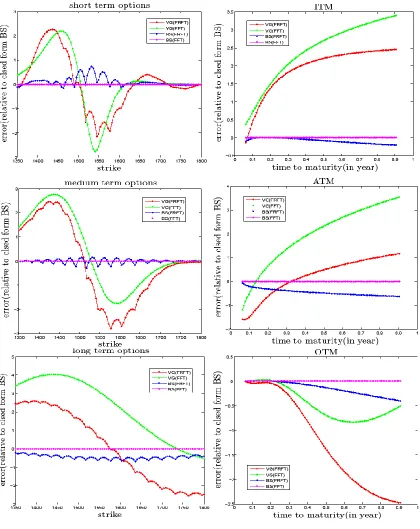
We now investigate the pricing errors for four model specifications BS(FRFT), BS(FFT),

VG (FRFT) and VG (FFT), across maturity and strike, relative to the closed-form

Black-Scholes prices. Our motivation is to examine the impact of the FRFT and FFT valuation

methods and the impact of the underlying models (BS vs. VG) on the option price.

To reveal cross-strike features of FRFT and FFT under the time changed and original

processes we express pricing errors as functions of strikes only, holding the maturity

constant. We consider three different maturities observed in the market: minimum, mean

and maximum corresponding to short, medium and long term options respectively:

ERRORmodel

 

K_i Pmodel



K_i ,t



PBS



K_i ,t



(74)

Similarly, to reveal cross-maturity features of FRFT and FFT we express pricing errors as

function of maturities only, holding the strike constant. Three different strikes are

considered: minimum, equal to asset and maximum of the observed strikes in the market;

ERRORmodel

 

t_i Pmodel

 

K,t_i PBS



K ,t_i



(75)

We plot cross-strike (left) and cross-maturity (right) errors, for different specifications, in

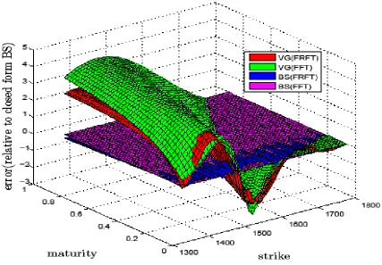
Figure 5 using illustrative market data for the last week of July 2007. Figure 6 plots error

surfaces across all ranges of strikes and maturities.

Three points stand out from these Figures. First, there is relatively little difference

between the FRFT and FFT estimates of the BS option prices. Second, FRFT and FFT

estimates of the VG option prices are often similar in pattern, but there are some notable

differences; moreover, the differences between FRFT and FFT estimates of VG option

prices seem to become more pronounced as we move down Figure 5 toward longer-term

options (on the left hand side) and OTM options (on the right). Third, there are (as we

would expect) pronounced differences between the BS and VG option prices. Put another

way, if the VG model is correct then the BS model will often give poor valuations: these

pricing errors are related (in complicated ways) to the options’ maturities and strikes or

moneyness.

[FIGURE 5 APPROXIMATELY HERE]

[FIGURE 6 APPROXIMATELY HERE]

7. Conclusion

In this study we have demonstrated how the standard Lévy–Kintchine formula can be

used to value options using an illustrative example of a Variance-Gamma process. Using

this derivation we have also been able to offer a correct solution to the mis-specification

in the Lévy measure for the VG model derived by Geman (2002). We also calibrated the

VG and BS models using weekly options data using both FFT and FRFT methods. We

found that the FRFT is much faster than the FFT approach, economizing on 97-98% of

the calculation time at the cost of small pricing errors; we also found that there are

important differences between BS and VG option values, implying that the inappropriate

use of the BS in a context where the true process was VG can lead to major pricing errors.

These findings have important implications for the calibration of options models and for

options risk management in general. This said, our work is limited in so far as we have

only considered the application of the Lévy–Kintchine formula to a relatively simple VG

process. Its application to more complex Lévy processes remains a topic for future study.

References

Applebaum D (2004). Lévy Processes and Stochastic Calculus. Cambridge University Press, Cambridge

Bailey D and Swartztrauber P (1991). The fractional Fourier transform and applications, SIAM Review, 33, 389-404.

Black F and Scholes M (1973). The pricing of options and corporate liabilities,Journal of Political Economy, 81, 637-659.

Carr P and Madan D (1999). Option valuation using the fast Fourier transform, Journal of Computational Finance, 2, 61-73.

Carr P and Wu L (2004). Time-changed Lévy processes and option pricing, Journal of Financial Economics, 71, 113-141.

Chourdakis K M (2005). Option Pricing using the fractional FFT, Journal of Computational Finance, 8, 1-18.

Cont R and Tankov P (2004). Financial Modelling With Jump Processes, Chapman & Hall/CRC Financial Mathematics Series.

Geman H, Madan D and Yor M (2001). Time changes for Lévy processes, Mathematical Finance, 11, 79-96.

Geman H (2002). Pure Jump Lévy processes for asset price modelling, Journal of Banking & Finance, 26, 1297-1316.

Kyprianou A (2006). Introductory Lectures on Fluctuations of Lévy Processes with Applications,Springer.

Lee R W (2004). Option pricing by transform methods: extensions, unification, and error control, Journal of Computational Finance, 7, 51-86.

Madan D Carra P and Chang E (1998). The variance Gamma Process and option pricing model, European Finance Review, 2, 79-105.

Merton R C (1973) Theory of rational option pricing, Bell Journal of Economics and Management Science, 4, 141-183.

Sato Ken-Iti (1999). Lévy Processes and Infinitely Divisible Distributions, Cambridge University Press Cambridge

Shiryaev A N (1999). Essentials of Stochastic Finance: Facts, Models, Theory, World Scientific.

[image:33.612.89.532.181.438.2]

Table 1: Calibration results under different specifications of Black-Scholes and Variance Gamma. We consider weekly traded options on S&P500 from January 2007 to November 2007. The estimates reported are the averages of dynamic weekly calibrations over this sample period. The standard error of each estimate appears in parentheses. The average (over 44 weeks) weekly calibration time is also reported.

Calibration Results

Specifications RMSE Average time (second) σ θ η

VG(FFT) 2.6931 20.97 0.1294 -0.1802 0.0786

VG(FRFT) 2.7234

3.1765

3.2447

3.1764

0.45

11.27

0.29

0.063

(0.0393)

0.1232

(0.0268)

-0.1837

(0.0221)

0.0839

BS(FFT)

(0.0505)

0.1320

(0.0313) (0.0276)

BS(FRFT)

BS(closed form)

(0.0360)

0.1308 (0.0362)

[image:34.612.95.517.166.337.2]

[image:35.612.94.518.127.311.2]

[image:36.612.91.516.182.368.2]

[image:37.612.92.520.127.311.2]

[image:38.612.95.515.182.711.2]

Figure 6: FRFT and FFT features under Variance Gamma and Black-Scholes models based on data for the last week of July 2007. The average spot was 1518.09

[image:39.612.104.531.132.429.2]