Flowfield dependent variation method for moving boundary problems

AIAA

JounNal

Vol. 53, No. 4, April 2015

Flowfield-Dependent

Variation

Method

for

Moving-Boundary

Problems

Mohd

Fadhli-University

Tun Hussein Onn

Malaysia,

86400 Batu Pahat,

Malaysia

Ashraf

A.

Omar+

University

of

Tripoli,

Sidy Almasry,

Al

Furnaj

Road,

Tripoli, Libya

and

Waqar

Asrat'

International Islamic

University

Malaysia,

50728

Kuala

Lumpur,

Malaysia

DOI: I 0.25 1411.J053353

A

novel numerical scherne using the combination

of

flowfield-dependent variation method and arbitrary

Lagrangian-Eulerian method is developed. This method is a mixed explicit-implicit nurnerical scherne, and its implicitness is dependent on the physical properties of the flowfield. The scheme is discretized using the finite-volume method to give flexibility in dealing with complicated geometries. The formulation itself yields a sparse matrix, which can be solved by using any iterative algorithrn. Several benchmark problems in two-dimensional inviscid and viscous flow have been selected to validate the method. Good agreement with available experimental and numerical data in

the literature has been obtained, thus showing its promising application in complex fluid-structure interaction problems.

4

b C;;

F

G

I,J

M

n Re

t U

um

f

O

?

d J

F.

6q 9

x

;

N

N

! r

!

'

Sa, Sb

s1, s2

sr, J4

Nomenclature

Jacobian of convection flux

Jacobian of diffusion flux

Jacobian of gradient diffusion flux

vector of convection flux

vector of diffusion flux

vertex index Mach number normal vector

Reynolds number

implicitness parameters

convection fl owfi eld-dependent variation parameters diffusion fl owfi eld-dependent variation parameters time

vector of conservative variables mesh velocity

spatial coordinate

control surface

control volume

I.

Introduction

[i

HE study of fluid phenomena is highly dependent on numerical

I

simulations because computational approaches are usually more economical. In fluid mechanics, such an approach is compu-tational fluid dynamics, and its development began with the advent

of

the computer

in

the 1950s. Continuous development

of

computa-tional power has enabled researchers

to

study

fluid flow

around

complete structures such as helicopters, airplanes, and spacecraft. However, algorithm efficiency of numerical solvers has become an issue as the size and the complexities

of

the problems increased. Moreover, muttidisciplinary problems such as moving-boundary or fluid-structure interaction problems become more relevant as the accuracy of the solution to the real-world application has becomes more demanding than ever before.

Recently, the so-called flowfield-dependent variation (FDV) meth-od has been developed [ 1] as an approach to solve complex fluid-flow

problems with a single numerical solver. Based on earlier works

of

Yoon and Chung [2] and Yoon et al. [3], the FDV method was devised by Chung I I ] to deal with a domain that contains all speed flows and various physical properties. The FDV method was formulated using the expansion of conservative variables in a special form of Taylor

series that included parameters that govern the implicitness of the

formulation. Furthermore, these parameters vary locally and made dependent on the physical properties of the flow instead ofpredeter-mined

like

other existing schemes and hence are named as FDV

parameters. In particular, these parameters are evaluated based on the local gradients of certain physical parameters such as Mach and Reynolds numbers in a computational domain. As a result, the FDV

method becomes a mixed

explicirimplicit

numerical scheme that

will

adjust accordingly for every computational point based on the

flow properties in that domain

Il-41.

Chung

[1]

applied finite-element method

to

approximate FDV formulation, but later Schunk et al. [5] addressed the FDV method as

a strategy toward unification

of

finite-element, finite-volume, and finite-difference methods. Spatial discretization is simply the option

to discretize between adjacent grid points or within an element but does not dictate the physics because all the physical phenomena are taken into account in FDVequations. Recently, Elfaghi et al. [6,7] has successfully combined the finite-difference form

of

FDV method

with higher-order compact method, which makes the method more

efficient in obtaining high-accuracy solutions. Moreover, the FDV

method has been expanded to high-energy astrophysics application

by

Richardson

et

al.

[8].

They found that the

FDV

method is Subscripts

i,

j,

k =

spatial dimension index Superscript

n

=

time level

Presented asPaper2O14-2689 at the 32nd AIAA Applied Aerodynamics Conference, Atlanta, GA, 16-20 June 2014; received 19 January 2014; revision received 14 June 2014; accepted for publication 28 August 2014; published online

I

December 2014. Copyright @ 2014 by the American Institute of Aeronautics and Astronautics, Inc. All rights reserved. Copies of this paper may be made for personal or internal use, on condition that the copier pay the $10.00 per-copy fee to the Copyright Clearance Centet Inc., 222 Rosewood Drive, Danvers, MA 01923; include the code 1533-385X/14 and $10.00 in correspondence with the CCC.

*Assistant _{Lecturet Department} of Aeronautical Engineering, P.O. Box

101 ; [email protected].

tProfessor, Department of Aeronautical Engineering, P.O. Box 81507; [email protected]. Senior Member AIAA.

lProfessot _{Department Mechanical Engineering, P.O. Box l0; waqar@} iium.edu.my.

FADHLI. OMAR. AND ASRAR t027

N

F

c

A

;

d

N

! o

,

numerically stable and comparable with Yee's total variation dimin-ishing (TVD) method [9] in terms of accuracy.

On the other hand, moving-boundary problems or fluid-structure

interaction problems are the cases where the structure interacts with its surrounding fluid through the movement of its boundaries or the shape and location of the original structue changes due to the effect of the fluid flow. Some examples are _{rotating Propellers,} wing flutter, parachute openings, flapping wings, accelerating aircraft or cars, re-ciprocating engines, vibration of suspension bridges, pulsating blood vessels, etc. Some movements of the boundary are relatively small,

but when they undergo large displacements, rotations, or deforma-tions, the effects offluid-structure interaction cannot be ignored. The need to solve such flow problems using dynamic mesh has attracted many researchers to develop various kinds

ofmoving-grid-interpola-tion techniques, and one ofthem is the arbitrary Lagrangian-Eulerian (ALE) method

_[0].

The ALE method was originally introduced in a

finite-difference formulation

[

1] and has been successfully

imple-mented in finite-volume (Xia and

Lin[12],

Guardone et al. [13] and Habchi et al.

_[lal)

and finite-element formulations (Feistauer et al. 115,16l and Sun et

al.

[l7]).

In

addition, many researchers have enforced the geometric conservation law (GCL) [18,19] due to the

influence

of

remeshing technique

in

the stability and accuracy

of

the ALE method. However, development of numerical schemes for moving-boundary cases

still

remain specifically

on

the physical properties of the goveming flows. For instance, the ALE application developed by Guardone et al. I I 3] and Feistauer et al. I I 6] is based on

the compressible flow model, whereas Xia and

Lin

[12], Sun et al. t171, and Habchi

et

al.

[14]

are based

on the

incompressible

flow model.

This paper proposes a novel technique based on a combination

of

the ALE and FDV methods as a way to overcome diffrculties when dealing with complex flow interactions due to the moving boundary. Our objective to extend the FDV method for multidisciplinary

appli-cations is motivated by the capability of the FDV method in dealing

with the transition and interaction of complex fluid flows. Although

some researchers have implemented the FDV method as an enor indi-cator for adaptive mesh refinement [20], to the authors' knowledge' to

date this method has not been fully incorporated into a fluid-structure

application that involves dynamic meshes.

Details of the FDV theory and the development of the

ALE-FDV

method for two-dimensional applications are written in Sec.

ll.

The

applicability

of

the

ALE-FDV

method

for

moving boundaries in

two-dimensional inviscid and viscous flow problems is demonstrated in Sec. III as well as the discussion about its accuracy and validity. We conclude the paper in Sec. IV. The ALE-FDV method is expected to provide a new technique

in

resolving the interaction

of

arbitrary

bodies in complex flowfields.

il.

Arbitrary

Lagrangian-Eulerian Form

of

Flowfield-Dependent

Variation Formulation

A.

Flowfield-DependentVariationMethod

Goveming equations

of

three-dimensional compressible

New-tonian fluid in conservative, dimensionless form (without the source term) can be written as

dU dF, N,

d,

+C+;: o

(1)

where the definition of vectors U , F , and G are given as

a:

Here,

p

and p are density and pressure (all flow properties and

quan-tities are dimensionless), respectively, and rz; is the velociry element

in

Cartesian coordinate.

E

and

t

are the total energy and intemal

energy per unit mass, respectively.

Re-

is the reference (e.g., free-stream) Reynolds number defined as

Re-

:

_P*V*L/lt*,

where

p

*,

V

*,

and

p*

are reference density, reference velocity, and

refer-ence dynamic viscosity, respectively; and

/-

is

the characteristic

length.

Pr

is the Prandtl number, and 7

is

1.4 for ideal gases. For

Newtonian fluids, viscous stresses z;; are proportional to the velocity

gradients:

I

dui

du

;\

_, dur,

-,,i:

_F\;*

_u")+

^-;;6u

(3)

where d,; is the Kronecker delta, p is the dynamic viscosity

coeffi-cient, and 2 is approximated as

)

:

_{-2 /3pbased} on Stokes's

hypoth-esis. Chung et

al. [1]

developed the

FDV

method

by

introduced parameters .rn and s6 into a special form ofTaylor series

ofconser-vative variables U and then applied the governing Eq. (1) into such a series. Consider the expansion

of

U

in

the special form of Taylor series up to the second-order time derivatives as

.

I

dll'

daun+r

_\

Auntt

_-

Orl

"

+t,

_dt

)

*ol(FL:*

r"

_"Y*')

+

o(Ar3)

(4)

' 2 \a1z '-D dr2 I -'

and second-order time derivatives of U as

&u dl. ...1

oFi

dGi\. dldFt

ac*\l

;l

:

-

_orl''i

+'')l-t;

-

₄

₎

*

""r\-'"

-'"

_/i

(5)

where AUn+l is defined as (Jn+t

_-

U',

and the Jacobians a;, D;, and c;; are defi ned a s dF i / dIJ, dG i / dU,

nd

0G i / @U

/ dx)'

respectively. Substinrting Eqs.

(l)

and (5) into Eq. (4), and assuming third-order

derivatives to be negligible, yields

. I

dF"'

dci

_[dAFl+r

dacl+r_]

_\

AU'-'-

o,l-;;-

_{d_,-}

_'"1

_a*,

*

_d,

₎₎

*ol(!,,,

_'

* b,t(dli-' *

{l'

')

2

_\dx"-'

'

-"\ dx;

dx1

|

()

|

d\Fi+t

aaGl+r

\

\

+srl(a,+r')l*++ll

(6)

' "dxi

'\

_dxj

_{dxj ll}

Parameters sn and s6 have a value between 0 and

I

and are called

implicitness parameters because the equation becomes fully explicit

if

both parameters are 0 or fully implicit if they are 1.

If

their values are between 0 and 1, they act as a weight factor between explicit and implicit equations. The principal idea

in

the FDV method is that

implicitneJs parameters are flowfield-dependent (i.e., calculated

auiomatically from physical changes in the flow instead

ofpredeter-mined manually to a single number irrespective of the variation of the

local flowfield). Therefore, within Eq. (6), parameters so and s6 are defined to be flowfield-dependent parameters and split into several convection and diffusion parameters s1-sa [1] as follows:

,"(lr+ac)

+s1AF*s.qAG

\/(7\

rr(ar'+

ac) +

s2AF

*

saAG

Parameters .T1 and s2 are named as first-order and second-order convection FDV parameters, whereas

si

alld J4 are named as

first-order and second-first-order diffusion FDV parameters, respectively' As shown

in

the following equation, convection and diffusion FDV

parameters are defined to be dependent on the gradient of the local Gi

le |

| Pui

I

I

ur'l

F,=

|

1,u,u1*

na,,

l.

LpEJ

L(pEIp)u,

J

:_rl :,

I

Re-l

'

I

lu1ri1

*

Up/Prl(dt/dx,\

)

FADHLI. OMAR. AND ASRAR

s2=1/2(7+s'l)

*

=

{''"1"'

Mach number and

local

Reynolds number, respectively, within adjacent computational nodes:

/ min(

r-.

₁₎

r.

>

a

I ^

/rn_;M*

sr: {

_'l

O

r,.<a

M^in*o.

,,:*:-

_'M

t

I

M^;n:O

rd)

a

r...a

Re-1nlo.

,r:J^6=^4"

_o

Rr^rn

Re-in:

o

sq:l/Z(r+

s\)

(8)

In Eq. (8), the constant o is chosen typically about 0.01, whereas 4 is

chosen appropriately between

0.05

and

0.2,

depending

on

the problem being solved [4,7]. For the sake of simplicity, ais set as 0.01 and 4 is chosen as 0.I for all problems investigated in this study. If the problem being solved involves high temperature gradients, such as in high-speed flows, the P6clet number can be used instead

of

the Reynolds number.

As a result, changing implicitness parameters

s,

and s6 in Eq. (6)

into FDV parameters through Eq. (7) yields

| /;rp,-,\

/aac,

_'\

|

aan+'

_-

-a/L,r,l?/

+':r|.?-/_l

-

I

T

/a.1P"-'

1

/aac;'

_\l

_\

*+

I

f,r+(',

+r')(?)

+

saft@i*

r,,(.=,.,

/.l,

-n,[gt*gql

*rLl

26,

+

b,)(o++Y)'l

*

olarr)

(e)

-AtLTii-1-

;tl r

2

L;trsr

T

",'\

d,,

T7t

)

)- "

Reananging the equation further by replacing unknown flux terms at time level n

+

1 with their associated Jacobians and assuming

third-order derivatives to be negligible yields the final form of the FDV

method:

A

a2

..

dou

AIJn+t

_ _i_tttO,d,U)tr+r _

_"_

(AlEi1LUl"

rr_Ar_=

dxi'

dx,dx

_i

''

dxi

(l0)

where

Di=spils3b;

A1

E;1

:

s{;1

_{-ito, }}

b)(s2a1+

sabl)

Q

=

Fi+c,-Llra,

+

b)*,Gt

+

G

j)

(11)

B.

Arbitrary Lagrangian-Eulerian Form of Flowfield'Dependent Variation Method

The fluid is described in an Eulerian manner in fluid mechanics because fluid particles are moving with respect to the fixed compu-tational mesh. In solid mechanics, however, the solid is described in a Lagrangian manner because each nodal point of the computational domain follows the movement of associated structures. The arbitrary

Lagrangian-Eulerian

(ALE)

technique combines Lagrangian and Eulerian descriptions ofa continuum (i.e., fluid and solid) in a single numerical scheme. As a result, ALE-type numerical schemes allow a

computational mesh

to

move arbitrarily as

well

as

following

adequately the movement of existing structues in the fluid' whereas the fluid is still seen in the Eulerian manner.

To apply the FDV method to solve moving-boundary problems,

we propose to develop the FDV method

in

an

ALE

formulation, which we name as the

ALE-FDV

method. In addition, because we

intend

to

make the proposed method applicable

in

solving flow

problems involving complicated geometries, we discretize

it

using the finite-volume method. To our knowledge, up to this point' the FDV method has only been formulated in the Eulerian manner. The

finite-volume

form

of

FDV

method can be obtained

by

volume integration of Eq. (10) over a conftol volume Q [41. Considering a

moving control volume at time instant t as Cl(t) and its boundaries as

f(t),

the integral form of FDV formulation is

f Altnll

fl

;

I

/

-Y-69: -

|

lp,r,ur

'r+j;tE,rAUl'tt +Q'l.ndl

J Lt

J

t

oxi

_)

o(0

f(r)

(t2)

Moreover, because the control volume is not fixed

in

space for a numerical method involving deforming mesh, the rate of change of a control volume mustbe taken into account. To determine scalar

quan-tities (i.e., density, pressure, and velocity components, etc.), inside

the control volume, ALE-type numerical scheme uses Reynolds's transport theorem [10] to connect the rate of change of the control volume

with

the changes

of

scalar quantities inside the control volume. Consider the boundary

of

the control volume

O(t)

move

with velocity

u.,

and q is a scalar quantity inside the control volume; Reynolds's transport theorem gives the time rate

of

change of the control volume as

N

o

;

N

o

3

)

o

*,

_o(r)

_Ito":

_c)(r)

I*da+

_r(4

lva,,'ndr

(r3)

Replacing rp with fluid density p, momentum

pr;,

and specific total Terey

nE,Eq. (13) can be rewritten in vector and semidiscrete form

Ll

_t

udo'l'-'

:

t^-y!de+

[I],u,n.ndr

r,4)

At

_l./

'r,r

- I

;{,,

at

!r,

The FDV method is applied by substituting the first term of the

right-hand side of Eq. (14) with the FDV formulation written in Eq. (12)' which yields

Ati

udo'l'-'

:

_-

flo,orr,

_'

+3rr,

i*Ir)n-,

At

_f,f

o,,r I

J,,L'

d,i

+

(Q

_-u'u))'ndr

(15)

Equation ( I 5) is linearized by applying the chain rule on the left-hand side term:

o[/,,,,r0n]

n*'

:

6s'*'[,/*,,

on]'.'

The right-hand side ofEq. (15) is linearized by lagging the

D

and E terrns one time step behind, which yields the ALE form of the FDV

method:

f t

'ln I

f f

d

LU"',1

_{I dol +tt}

_{llD,(LIJtn-t-Eij+\Lllta-t}

_l.zdr:

LJout

J

J

t'

'oxi

J r(r)

r

f f

1nl

-N

_{J _}

l(Q'^-Il"a,,l-ndl-IJ'al

.

_L,/oul

I dol

_I

(l'll

I-(1)

Equation (17)

is

applicable

for

three-dimensional

flow

problems, and any standard finite-volume technique can be used to discretize

the volume and surface integrals

in

it.

However

in

this paper, the application of the ALE-FDV method is focused on two-dimensional moving-boundary problems, and we adopted vertex-centered

finite-+u'a[/

,',ao]"*'

r(J-r)

..,-,

_o

ac&r)

?

N

;

s.

d

s

;

N

r

F

o

I(J+r)

{x)

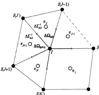
Fig.

I

Deffnition of cell I for vertex-centered finite volume.

volume method to discretize Eq. (17). Vertex-centered finite volume was chosen because the implementation of the wall-boundary condi-tion can be defined explicitly (e.g., the velocity of the flow on some pointof thewall is same as the wall velocity of thatparticularpointfor moving-boundary problems) without using some additional points, as in the case ofcell-centered finite volume, where usually additional cells called ghost cells are used to apply the wall-boundary condition.

Consider a vertex 1 surrounded by several triangular and quadrilat-eral elements €"/, as shown in Fig. 1. The cell (i.e., control volume)

of

vertex 1 is defined by joining centroid of its surrounding elements' Face Al117,l

or

Af7,7;2

is

formed either

by

connecting centroid element e7 or element ey11 with the median of line connecting vertex 1 and its neighbor vertex 1(J). On the other hand, the subvolume

of

cell

/,

AC)n7,, is formed by joining the median of line 1

-

I(J

-

l),

centroid elements e7, the median

ofline

1

_-

1(J), and vertex 1.

Based on Fig.

I, ALE-FDV

formulation can be discretized as

FADHLI, OMAR, AND ASRAR

b) t ₌ 0.57

Fig.

2

Motion of the deformable mesh.

In

Eqs. (18) and (19), interface variables can be approximated by

using the centroid value of adjacent cells. Because interfaces values are defined at the median ofline

/

_-

1(,/), as shown in Fig. l, interface

variables can be easily determined

by

the average between two

connecting cell centroid values. On the other hand, the gradients of

interface variables can be approximated by either the technique called least-square gradient reconstruction (LSGR) method [21] or by the Green-Gauss method [22] as follows:

(20)

where,

in

two-dimensional space,

V is

a

small area where the interface value O resides, and S is the boundary or perimeter of such an area.

In

this

study, we adopted the Green-Gauss method to approximate the gradient

of

interface

AU

[third term

in

Eq. (18)] because

it

is

much simpler than the LSGR method that requires

matrix manipulation. For example, in Fig. 1, the gradient of interface

AU at the median of line 1

_-

1(,D (i.e., AU7) is determined by taking

V as the combined area of two adjacent elements e7 and e711, and @

is

the

average value

of AU

at

each boundary dS, namely line

I

_-

I(J

_-

r),

I(J

_-l)

_-1(/),

I(J)

_-

r(J

_*

1), and

I(J +

I)

-

I.

Similarly, the interface gradient

of

the velocity as

well

as the

intemal energy

in

the viscous

flux

G;

are interpolated using the Green-Causs method. On the other hand, the inviscid

flux

F;

is approximated as the numerical

flux

by the high-order monotonic upstream-centered scheme for conservation laws (MUSCL) scheme for the unstructured grid [23], as shown in

_fu'

(21), instead of taking

an average

of

analytical

flux

between two cell centroids, which is

only first-order accurate: I

(F

_-

IJu,,) .

_n

:

:(F(Uil

₊

F(U

)

_-

(Un

+

U)a.)'

n

L

(21)

aul.'[iaon,,]'*'

*o,f

_["i

(oo)'.'

where known terms on the right-hand side are

N TN 1n*l

n,

:

_-ar

_I

l(Qn

-

rl^

u.l'

n AFl,,r,

_-

ui

LII

aor,r,

I

,1 Ll:t J

(1e)

In

Eq. (21),

A

is the convection Jacobian matrix evaluated based on Roe's average properties, and 1 is the identity matrix. lnterface gradients of fluxes

in

_Q

li.e.,

d/dxi

(F

_i

*

Gi) in

Eq' (11)l can be approximated by averaging the gradients of fluxes in cell 1 and its adjacent cell 1(,/), as shown in Fig. l, where gradients in each cells are determined by the Green-Gauss method using the

F;

and G; at the

cell interfaces. Besides conservation laws of mass, momentum' and energy, the geometric conservation law (GCL) [18] is required for

ALE+ype

numerical schemes.

To

make

the

formulation

GCL-compliant, the cell volumes in Eqs. ( I 8) and ( 19) are evaluated by its boundary velocity as follows:

n

^r

+

Eir(*or)'*'

"^.],,,,

l,l;

(*.),

:i1,"

,*

-|to(o^,r,,,)

-

r(,^

_")rcan-'L)

ofion,]".'

:

_^'[Ei(,.,

n)ory,,,f"*"'

(22)

Finally, the resulting equation wriften in compact form is

[image:4.596.52.255.49.243.2]

i030

Table

I

Velocities maximum error norm

L*

(a;)

Time

L^

(u,l

L-

(ut)

0.5r

1.338

-

15

1.948

-

ls

T

l;7'7E

-

15

1.448

_-

15

K _t LU',;+ r + r</1 r )

AUIIi

+

... ₊ K _r

_o

LU',;[,'

+

...

_+Kr,",

A U

_it

\

:

R, (23\

where K7 and Klgy denote the collective sum of contributions for

the main cell and its surrounding cells, respectively. As far as the unstructured mesh is concemed, combining Eq. (23) for all cells in the computational domain

will

result in a linear system of equations

with large sparse matrix, namely

[Kl:

Lrl[au'+r]:

LRI (24)

To solve the linear system of Eq. (24), we used an iterative method: the restart general minimal residual (restart GMRES) algorithm [24]. In addition, restart GMRES is combined with the left-block Gauss-Seidel preconditioner [25 ] to accelerate the convergence of solutions.

Although other preconditioners that converge faster exist, the

Gauss-Seidel preconditioner was chosen because it is relatively simple.

III.

Results

and

Discussions

A.

FreestreamPreservation

To verify whether the

ALE-FDV

method satisfied the GCL, we conducted a freestream preservation test on a mesh that deformed like

a wave, as depicted in Fig. 2. The mesh is a square domain with a size

of

I

x

I

unit squared, and as shown in Fig. 2a, the mesh has initially 5 12 uniform triangular elements. The motion of the mesh is defined as [261

x':*t:xilaxi

(2s)

with I

:

l,

2

for two-dimensional cases. The amplitude

A; is

set as 0.1; the reference length

L;

and time

I

are set as 1.0 and 20, respectively; constants c

_I

and c ₂ are 4n ; and constant cr is z. The test has been performed using a time interval

Al

:

0.01. Inviscid uniform flow (a 1

:

1.0, uz

:

0) was set as an initial and boundary condition.

The solution was advanced in time until r

:

7, where the mesh is at its maximum distortion, as depicted in Fig. 2c.

Results of maximum error norm

L-

of velocities u _; and a2 at time instant r

:0.5T

and

r:

Z

are reported

in

Table

l.

The present FADHLI. OMAR. AND ASRAR

Ax;(r)

:

^o,(+),'"(,,

fr),"("

fr),'"('?)

Fig.5

mesh. 0.1

-0.1 a

N J

t"

b:

;

N

N

E

r

F

4.2

6

o.s

-0.4

-0.5

-0.6

-0.7

exact

-Sua4

E

tna

Ie-05

l0

1000

Cornparison of density error between deformed and stationary

le-00

le-01

le-02

I F ar1

le-03

le-04

-1.5

-l 4.5 0 0.5 I

1.5

2

x

Fig.3

Comparison between exact solutions and numerical solutions of

pressurecoefficientalong.r2

_{= 0atJ =}

0.1.

100

\iN

"'ti

{il

b) Triangular mesh

Fig.4

Density contour at time

I

₌

0.1.

L@(quad-strD

+

L2

(quad-sta0

-l-L6

(tri-stat)

-+-L2

(tri+taO

--L-Lo(quad-move)

g-L2 (quad-move)

-€]-Lo

(tri-move)

+

\

8:::;;;gi.$

[image:5.596.307.524.315.522.2] [image:5.596.49.267.316.526.2]

FADHLI. OMAR. AND ASRAR t 031

(26)

results show that the

ALE-FDV

method has errors around 10-15, which is closed to machine zero for double-precision computation. Therefore, freestream preservation is achieved, and the

ALE-FDV

method is verified to be GCl-compliant.

B.

Propagating Isentropic Vortex

The accuracy ofthe proposed ALE-FDV method for a deformable mesh is verified by the following, propagating isentropic vortex in

two-dimensional inviscid flow. Initially, the flows are perturbed by an isentropic vortex centered at (0,0). The perturbed values ofvelocity,

density, and pressure are given l26,27lby

a) -1.84 deg (Pitching up)

c) 1.47 deg (Pitching up)

u^,f,

"*vlr/r(t

-#))

lt

-

rrr<r-

r)uh".

*n

(t-

#))"'-'

il

N J

F

c

I

;

N

! r

!

U,:

P,:

P,:

l/YPl

where

r

is

the radial distance

of

any point

in

the computational domain from the vortex center at time ,, and U.u* is the maximum velocity at distance

r

:

b.The radial distance r is defined as

.&

_t*

f,

|

_\iltr

,e

t

d) 0.02 deg (Pitching down)

FADHLI. OMAR. AND ASRAR

-

Uur)2

a

(x,

-

Votl2

r=

(27)

The exact solutions are then given by

(28)

tindon [28]

r

Venkatakrishnan and Mavriplis [30] O present

--2-l0l

Angle of attaclg deg Fig.

7

Comparison of lift

coefficient-01020304050

Angle ofattack, deg

Fig.8

Comparison

oflift

coelficent c1 and drag coefficient c7.

Table

2

Summary of unstructured meshes

Name

Nodes

Smallest element size

Coarse

12,9W

Medium

18,570

Fine

24.170

0.00048 0.00036 0.00025

l'r,l:l

y'

l.l:,::::l

tpJ

L0J

L p, I

o

9a

I 0.5

0.25

0

4.25

i.e., the vortex

will

retain its shape while convecting in the domain

with freestream velocity (U6, Vs) through time. The initial condition is given by Uo

:0.5,

y0

:

0.0, U-u"

:

O.SUy, and b

:0.2.

The computational domain is set as 4 x 4 unit squared, centered at (0' 0).

Two kinds

of

mesh are employed

in

this case, namely uniform quadrilateral

and uniform

triangular mesh,

to

demonstrate the applicability

of

the proposed method for unstructured mesh. Both

kinds of mesh are deformed in time by the motion defined in Eq. (25). In this case, the amplitude A; is set as 0.2; the reference length L; and dme

f

are set as 4.0 and 0. l, respectively; constants c

_I

and c2 are

2t;

and the constant c, is

r.In

addition, similar to [26], a very small time interval is chosen

(At

:

5

x

l0-5)

to eliminate the effect

of

time

integration

eror

on the accuracY.

The accuracy of the proposed method is analyzed at time instant

t

₌

0.1 because the mesh has the largest deformation at this time

regardless

of

the type

of

the mesh. Numerical results

of

presswe

coefficient

c,

for both meshes are in good agreement with the exact solution, as shown in Fig. 3. On the otherhand, as shown in Fig.4, the

vortex as depicted by the density contour for the triangular mesh Gig. ab) qualitatively preserves its shape better than the vortex in a quadrilateral mesh (Fig. 4a). However, both meshes do not preserve the shape of the vortex exactly as predicted by the exact solution (i'e., a circular shape) due

to

the dissipation effor

of

the second-order

MUSCL scheme used

in

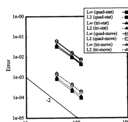
the proposed method. Furthermore' the numerical error ofthe density distribution in terms ofaverage squared error norrn L2 and maximum error norm

L-

for three different grid

resolutions with the number of nodes

N

:

1600, 64OO' and 14,400 are plotted in Fig. 5. As a comparison, the errors for a stationary mesh are plotted in the same figure. Overall, slope ofthe errors for each case is close to

_-2,

implying that the method is second-order accurate in

space.

In

particular, the enors produced

by

the quadrilateral and triangular meshes are the same, but the errors due to the motion of the mesh are slightly higher than the stationary mesh.

C.

Oscillating NACA 0012 Airfoil

This case was first investigated experimentally by Landon [28] and since then has been used

by

many researchers as a benchmark

problem

to

validate numerical solutions

of

moving bodies inside

inviscid compressible flows. ln this case a NACA 0012 airfoil which

oscillates harmonically about its quarter chord in a flow with free

stream Mach number

M

:0.75

is

considered'

The

oscillating motion is defined by the angle-of-attack function:

vorticity 100

to

I

-100 a

d

;

P d

{

I

;

N

= N

€

,

4.5 L -J

Vorllcfty

lfn

t

]

:

=0

t

_-lm

{}

b) Schneiders et al. [31, Fig.

9

Comparison of vorticity profile at 44 deg angle of attack.

o

Visbal and Shang [33]

----

Lomtev etal. [34]

---

Schneiders et al. [31]

-

present

[image:7.595.36.279.59.553.2]

FADHLI. OMAR. AND ASRAR 1033

a(t)

:

6.616

*

2.51 sin(urt) (2e)

where the angular velocity is given by ur

:

2kU _{* /} c, and the reduced frequency is k

:

0.0814. The numerical simulation was conducted

by using an unstructured mesh with 6700 cells. To properly capture the shock, the MUSCL scheme for the unstructured mesh combined

with minmod _{limiters [23]} has been used to approximate the inviscid flux. Figure 6 shows the instantaneous pressue contour around the airfoil at several angles

of

attack. The strength of the shock wave decreased, and its location shifted from the lower to the upper surface as the airfoil pitches up, qualitatively similar to the results shown by

Murman et al. [29].

As shown in Fig. 7, the hysteresis of the lift coeffrcient obtained by

the present method is in good agreement with the numerical solutions reportedby Venkatakrishnan and Mavriplis [30] and Schneiders etal.

[31] butlack agreement with the experimental results of Landon [28j. The discrepancy between numerical and experimental data is perhaps due to the viscous effect of the flow in the experiment. Mohaghegh and Jafarian _[32] reported that the interaction ofthe boundary layer and the shock wave produced by the airfoil has reduced the strength

of

the shock compared

with

the inviscid simulation, resulting in

a)t=3.5

differences between experimental data

and inviscid

numerical solutions.

D.

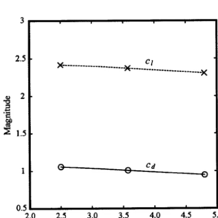
Rapirlly Pitching NACA 0015 Airfoil

In this section, we consider a laminar viscous flow past a NACA 0015 airfoit that is pitched rapidly from 0 deg angle of attack at a constant pitch rate:

'a7

:

,olt-

*n(-.uf11

about the axis located at the quarter-chord. The final pitch rate is set as rll0

:

0.6, and the time taken by the airfoil to reach 997o of ar6 is given

by f0

:

1.0. The freestream Mach number and Reynolds number are

M

:

0.2 and Re

:

10,000, respectively. The numerical simulation was conducted using an unstructured mesh with 28,134 grid points.

This case was first studied by Visbal and Shang [33] and later was used for validation of numerical solutions by Lomtev et al. [34] and Schneiders et al. [ 3 I l. Figure 8 shows the comparison of drag and

lift

coefficients obtained by the present method with others. The uends

of

(30)

N J

o

E

A

=

;

N

F

N

q

t

c) r = 15.0

[image:8.596.128.445.291.728.2]

i034 FADHLI. OMAR. AND ASRAR

,t::11-:i

[image:9.596.123.445.48.492.2]

\l\.).,':

Fig.11

ar

₌

3.0 Qeftfigures: present' rightfigures: Sen etal. [35]).

:

;

@

G'

c

A

;

N

r

'

b)l=3.0

c)t=5.0

1ift and drag coefficient from the present results match quite well with those available in the literature.

The vorticity profile at 44 deg angle

of

attack obtained

by

the proposed method is shown in Fig. 9a. As a comparison, Fig. 9b also shows the sarnevorticity results obtainedby Schneiders etal. [31 ]. Both figures show a similar pattem of vortex strucnues such as the leading-edge vortex and traiting-edge vortex detached from the airfoil and several shear-layer vortices existing on the upper surface of the airfoil'

E.

Rotating Cylinder

In

this problem, a laminar viscous flow with Re

:

1000 past a circular cylinder that rotates impulsively from rest is considered. Two angular speeds are used:

ro:

1.0 and

a:3.0.

The unstructured mesh with 18,570 cells was used for both cases. In addition, for the

purpose

of

the grid-independence study,

two

other meshes with different number

of

cells were generated from the original mesh. Information on all meshes is summarized in Table 2.

[image:9.596.138.438.613.739.2]

a) Coarse mesh

FADHLI. OMAR. AND ASRAR

b) Fine mesh Fig.

13

Florvfield at

I

=

8.0 for case ar

=

1.0.

2.5

ot2

'o

o0 6t

E

r.s

N

;

;

po

5

9

H

;

N

N

F

!

t

o

0.5

x---'-'--'-"""*"x""-':-l---*.x

applications, motivated

by

an interest

to

extend

its

capability to

complex fluid-structure interaction, and the formulation is

discre-tized using vertex-centered finite-volume method. Two cases

of

prescribed boundary motion in inviscid flow and another two cases in

viscous flow have been chosen as benchmark problems to validate the

ALE-FDV method. The results obtained are in good agreement with

other numerical/experimental methods, thus confirming its

applica-bility in solving moving-boundary problems.

References

[l

Chung,

T.

J., "Transitions and Interactions

of

Inviscid/Viscous, Compressible/Incompressible and Laminar/Turbulent Flows," lnterna-tional Journal for Numerical Methods in Fluids, Vol' 31' No. 1, 1999' pp.223-246.

doi: I 0. I 002/(ISSM I 097-0363

[2] Yoon, K. T., and Chung, T. J., "Three-Dimensional Mixed Explicit-Implicit Generalized Galerkin Spectral Element Methods for High-Speed Turbulent Compressible Flowsl' Computer Methods in Applied Mechanics and Engineering, Vol. I 35, No. 3, 1996, pp- 343-361

-doi: I 0. 10 I 6/0045-7825(96)01 066-3

[3] Yoon, K. T., Moon, S. Y, Garcia, S. A', Heard, G. W., and Chung' T. J.' "Flowfi eld-Dependent Mixed Explicit-lmplicit (FDMEI) Methods for High and Low Speed and Compressible and Incompressible Flows"' Computer Methods in Applied Mechanics and Engineering, Vol. 151' No. 1, 1998, pp.75-lM.

doi:1 0.1 0 I 6/50045-7825(97)00 I 1 4-X

[4] Chung, T. J., "Computational Fluid Dynamics ]' Cambridge Univ. Press, New York, 20O2, Chaps. 6, 7.

[5] Schunk, G., Canabal, F., Heard, G., and Chung, T. J.' "Unified CFD Methods Via Flowfield-Dependent Variation Theory," 30th Fluid Dynamics Conference, AIAA Paper 1999-3715, June-July 1999.

[6] Elfaghi, A. M., Asrar, W., and Omar, A' A., "Comparison of High-Order Accurate Schemes for Solving the Nonlinear Viscous Burgers Equa-tionl' Australian Journal of Basic and Applied Sciences,Yol.3, No' 3'

2009, pp. 253G2543.

[7] Elfaghi, A. M., Asrar, W., and Omar, A. A., "Higher Order

Compact-Flowfield Dependent Variation (HOC-FDV) Solution

of

One-Dimensional Problems," Engineeing Applications of Computational Fluid Mechanics, Vol. 4, No. 3, 2010, pp.

43U40.

doi: I 0.1080/19942060.2010.1 10 15330

[8] Richardson, G. A., Cassibry, J. T', Chung, T. J.' and Wu' S. T., "Finite Element Form of FDV for Widely Varying Flowfields," Journal of Computational Pftysics, Vol.229, No' 1,2010' pp. 145-16'7. doi: 1 0. 10 1 6/j jcp.2009.09.O23

[9] Yee, H. C., 'A Class of High-Resolution Explicit and Implicit Shock-Capturing Methods," NASA TM-101088, 1989.

[10] Donea, J., Huerta, A., Ponthot, J. P., and Rodriguez-Fenan'

A'''Arbi-trary Lagrangian-Eulerian Methods," Encyclopedia of Computational Mechanics, edi@d by Stein, E., Borst, R. D', and Hughes, T. J. R., Vol. I _'

John Wiley & Sons, New York,2004, pp' 1-25, Chap. 14.

tl 1l Hirt, C. W., Amsden, A. A., and Cook, J. L., 'An Arbitrary Lagrangian-Eulerian Computing Method for All Flow Speeds," _{"/oumal of Compu'} tational Physics, Vol. 14, No. 3, 1974, pp- 22'7-253.

doi:10.101 6/0021-999 1(74)9005 I -5

ll2l

Xia, G., and Lin, C. L.,'An Unstructured Finite Volume Approach for Structural Dynamics in Response to Fluid Motionsl' Computers and Structures, Vol. 86, No.7,2008, pp. 684-701'

doi: I 0. 1016ij.compstruc.2007.07.008 2.0

2.3 3.0 3.5 4.0 4.5

5.0

Element size

(x

104)

Fig.

14

Average lift and drag coellicient of each mesh for case ar

=

1.0'

Comparisons of the flowfield obtained using the medium-sized

cells with the results

of

Sen et al.

[35]

are shown

in

Fig.

10 for

a

:

1.0 and Fig. 71 for

ro:

3.0. Overall, both results agree quali-tatively. However, one can see some minor differences, such as at

t

:

8.0

in

Fig. 10, where the utmost right vortex is weaker' and at

t

:

1.5 in Fig. 11, where the location

of

a vortex near the cylinder surface is unmatched and the formation ofa secondary vortex does not

exist when compared

to

the results

of

Sen

et al.

1351. Neverthe-less, similar flowfield sffuctures can be observed by comparing the curent results (t

:3.5, co:

1.0 and

t

:

5.0,

a:3.0)

and the experimental results of Badr et al. [36], as shown in Fig. 12.

Next, we compare the results of the case of ar

:

1.0 with the results obtained using the coarse mesh and the fine mesh.

As

shown in

Fig.

13, the coarse mesh and fine mesh gave a similar pattem

of

flowfield,

with

the results

of

the medium-sized mesh shown in Fig. 10b, indicating that all meshes gave consistent results. Figure 14 shows plot ofthe averaged

lift

coefficient c1 and the drag coefficient c2 vorSUS the smallest element size ofeach mesh. The average c/ and

c/

were determined based on the time period of r

:

5.5 to

t

:

15.0. The plot shows that good linear grid convergence with small differ-ences of c1 and c7 from all meshes is obtained. Therefore, we can conclude that the effect of the mesh on the results is small, and the solutions obtained by the medium mesh shown in Figs. l0 and l

l

are grid-independent.

IV.

Conclusions

The

capability

of

the ALE-FDV

method

in

solving

[image:10.596.127.443.49.198.2] [image:10.596.47.266.215.434.2]

I 036

[13] Guardone, A., Isola, D., and Quaranta, G., 'Arbitrary Lagrangian Eulerian Formulation for Two-Dimensional Flows Using Dynamic Meshes with Edge Swapping," Journal of Computational Physics, Vol. 230, No. 20,201 I, pp.7706-7722.

doi: 1 0. 10 16/j jcp.20l 1.06.026

ll4l

Habchi, C., Russeil, S., Bougeard, D., Harion, J. L., kmenand, T,

Ghanem, A., Valle, D. D., and Peerhossaini, H., "Partitioned Solver for Strongly Coupled Fluid-Structure Interaction," Computers & Fluicls, Vol. 71, Jan. 2013, pp. 306-319.

doi: 10. I 016/j.compfluid.20l 2. 1 1.004

[5]

Feistauer, M., Hasnedlov6-Prokopovii, J., Horddek, J., Kosik, A., and Kudera, V., "DGFEM for Dynamical Systems Describing Interaction of Compressible Fluid and Structures," Joumal of Computational arul Applied Mathematics, Vol. 254,Dec. 2013, pp. 17-30.

doi: I 0. 1 016/j.cam.20i 3.03.028

[16] Feistauer, M., Kudera, V., and Prokopov6, J., "Discontinuous Galerkin Solution of Compressible Flow in Time-Dependent Domainsi' Mathe-matics and Computers in Simulation, Vol. 80, No. 8, 2010, pp. 1612-1623.

doi: 1 0. 10 16/j.matcom.2009.01.020

I

l7]

Sun, X., Zhang, J. 2., and Ren, X. L., "Characteristic-Based Split (CBS)

Finite Element Method for Incompressible Viscous Flow with Moving Boundaries," Engineering Applications

of

Computational Fluid Mechanics, Vol. 6, No. 3,2012,pp.461474.

[i8]

Thomas, P. D., and Lombard, C. K., "Geometric Conservation Law and Its Application to Flow Computations on Moving Gridsi' AIAA Joumal, Vol. 17, No. 10, 1979, pp. 1030-1037.

doi:l0.2514/3.61273

t19l Guillard, H., and Farhat, C., "On the Significance of the Geometric Conservation Law for Flow Computations on Moving Meshes"' Com-puter Methods in Applied Mechanics and Engineering, Vol. 1 90' No. I I ' 2000, pp. r46't-1482.

doi:1 0. I 016/50045-7825(00)001 73-0

t20l Heard, G. W., "Flowfield-Dependent Variation (FDV) Method for Compressible, Incompressible, Viscous, and Inviscid Flow Interactions with FDV Adaptive Mesh Refinements and Parallel Processing," Ph.D. Dissertation, Univ. of Alabama, Huntsville, AL,2OO7 .

[2ll

Versteeg, H. K., and Malalasekera, W., An Introduction to Computa' tional Ftuid Dynamics: The Finite Volume Method, Pearson Education, Harlow, England, U.K., 2007, pp. 321-323.

[22] Diskin, 8., Thomas, J. L., Nielsen, E. J., Nishikawa, H., and White' J. A.'

"Comparison of Node-Centered and Cell-Centered Unstructured Finite-Volume Discretizations: Viscous Fhtxes," AIAA Journal, Vol' 48, No. 7' 2010, pp. 132G1338.

doi:'tO.251411.4494O

[23] Darwish, M. S., and Moukalled, F., *TVD Schemes for Unstructured Gids)' Intemational Journal of Heat and MassTranslea Vol. 46' No. 4' 2003, pp. 599-6 1 1 .

doi:1 0. 10 1 6/5001 7-93 l0(02)00330-7

[24] Saad, Y., and Schultz,

M.

H., "CMRES:

A

Generalized Minimal Residual Algorithm for Solving Nonsymmetric Linear Systems," SIAM Joumal on Scientific and Statistical Computing, Vol. 7, No' 3' 1986' pp. 856-869.

doi:10.1 I 3710907058

[25] Persson, P O., and Peraire, J., "Newton-GMRES Preconditioning for Discontinuous Galerkin Discretizations of the Navier-Stokes Equa-tions," SIAM Journal on Scientific Computing, Vol. 30, No' 6' 2008' pp.2709-2733.

doi: 10. I I 371070692108

t26l Yu, M. L., Wang, Z. J., and Hu, H., 'A High-Order Spectral Difference Method

for

Unstructured Dynamic

Gidsl'

Computers

&

Fluids, Vol. 48, No. l, 201 I, pp. 84-91.

doi: I 0. 1016/j.compfluid.20l 1.03.015

t27l Hu, R Q., Li, X. D., and Lin, D. K.,'Absorbing Boundary Conditions for Nonlinear Euler and Navier-Stokes Equations Based on the Perfectly Matched Layer Techniquel' Joumal

of

Computational Physics, Yol.227 , No. 9, 2008, pp. 43984424.

doi: 10. 10 l6ljjcp.2008.01.010

[28] Landon, R. H., "Compendium of Unsteady Aerodynamic Measure-ments," AGARD Rept. 702, Neuilly sur Seine, France, 1982.

[29] Murman, S.

M.,

Aftosmis,

M.

J., and Berger,

M.

J., "lmplicit

Approaches for Moving Boundmies in a 3-D Cartesian Method," 41st Aerospace Sciences Meeting and Exhibil, AIAA Paper 2003-1119' Jan. 2003.

[30] Venkatakrishnan,

V,

and Mavriplis, D. J., "lmplicit Method for the Computation of Unsteady Flows on Unstructured Gidsi' Joumal of Computational Physics, Vol. I 27, No. 2, 1996, pp. 380-397. doi: 10. I 006/jcph .'t996.0182

[31] Schneiders, L., Hartmann, D., Meinke, M., and Schriider,

W,

'An Accurate Moving Boundary Formulation in Cut-Cell Methods," Joar-nal of ComputatioJoar-nal Physics, Vol. 235, Feb. 2013' pp. 78G809. doi:10. l0 16/jjcp.20 12.09.038

[32] Mohaghegh, M. R., and Jafarian, M. M., "Unsteady Transonic Aerody-namic Analysis for Oscillatory Airfoils Using Time Spectral Method"' Intemational Joumal of Mechanical and Materials Engineering,Yol.

l,

No. 4. 2010. pp. 264-27 l.

l33l Visbal, M. R., and Shang, J. S., "Investigation of the Flow Structure Around a Rapidly Pitching Airfoil," AIAA Joumal,Yol. 27' No. 8' 1989' pp.104ut-1051.

doi:10.2514/3-1O219

[34] Lomtev, I., Kirby, R. M., and Karniadakis, G. E.'

'A

Discontinuous Galerkin ALE Method for Compressible Viscous Flows in Moving Domains," Journal of Computational Physics,Yol. 155' No'

l'

1999' pp. 128-159.

doi: 10. 1 006/jcph. I 999.633 I

[35] Sen, S., Kalita, J. C., and Gupta, M. M.,

'A

Robust Implicit Compact Scheme for Two-Dimensional Unsteady Flows with a Biharmonic Stream Function Formulation," Computers

&

Fluids' Vol. 84' Sept' 2013, pp. 141-163.

doi: 10. l0 I 6/j.compfluid.20l 3.05.016

t36l Badr, H. M., Coutanceau, M., Dennis, S. C. R., and Menard, C''

"Unsteady Flow Pasta Rotating Circular Cylinder at Reynolds Numbers 103 and 10a," Joumal of Fluid Mechanics,Yol.220' No' 1' 1990'

pp.459484.

doi : 1 0. 1 0 I 7/500221 120900033 42

Z.J.Wang

Associate Editor

FADHLI. OMAR. AND ASRAR

'r

d

;

;

ii

;

;

N

N

! r

€