Journal of Chemical and Pharmaceutical Research, 2014, 6(3):113-121
Research Article
CODEN(USA) : JCPRC5
ISSN : 0975-7384
The research of how to identify the computer network fault by improving
neural network
Hongbo Shao
1*, Lianjie Dong
1and Jianhui Wu
21College of Science, Agricultural University of Hebei, Baoding, China
2Hebei Province Key Laboratory of Occupational Health and Safety for Coal Industry, Division of Epidemiology
and Health Statistics, Hebei United University, Tang Shan, China
_____________________________________________________________________________________________
ABSTRACT
Computer network is one of the most important equipment in the whole world, with the gradual and rapid development of its scale, how to manage and maintain the computer network is becoming more and more complicated. The network fault diagnosis has become people’s focus. With the development of artificial intelligence, by introducing neural network technology into the area of network fault diagnosis, neural network can bring out its advantages in the fault diagnosis. This article would employ SOM neural network and BP neural network, the samples would be clustered by using SOM neural network, and the results of the cluster would be put back into the original samples, which would also be set with certain weights, through the weights’ consistent updating, the convergence speed of BP neural network can be improved. Through using LM algorithm to improve BP neural network and using computer network diagnosis as practical samples to simulate and analyze computer, the validity of this method has been proved, and at the same time building a system of computer network diagnosis can be very meaningful for theoretical study and practical use.
Keywords: Computer network diagnosis; neural network; Self-Organizing Feature Map neural network; Back-Propagation neural network; Levenberg-Marquardt algorithm
_____________________________________________________________________________________________
INTRODUCTION
Research background and current status
status identification.
After years’ development, the technology of fault diagnosis has been through three phases: Due to simple equipment, first phase mostly relied on main experts or maintenance staffs’ sensory organs, personal experience and simple instrument and worked out well [2]. The development of sensor technology, dynamic testing technology and signal analysis technology made the fault diagnosis technology go into the second phase, and all of the technologies have been widely used in the maintenance projects and reliability projects. In the early 80s, because equipment become more and more complicated, intelligent and integrated, traditional fault diagnosis technology cannot be adopted, with the development of computer technology, artificial intelligence and especially the experts system, fault diagnosis went into the third phase——the intelligence stage. Intelligent fault diagnosis technology includes fuzzy technology, Grey Theory (GT), Pattern Recognition (PR), Fault Tree Analysis (FTA), Diagnostic Expert System (DES), and so on. The previous four technologies only used logical reasoning knowledge in certain level and partly solved some problems in the process of diagnosis, such as fuzzy information, incomplete information, fault category and fault location; but DES can combine all other technologies and form hybrid intelligent fault diagnosis system by using itself as a flat. Neural network, which owns strong ability to adapt and to learn, has been widely used in many different areas, and been proved that it can solve many problems that traditional method cannot [5]. The particular nonlinear information processing adaptability of neural network has overcome the shortages of traditional artificial intelligence on instincts, such as pattern, speech recognition, and unstructured information processing, which explains the reason it has been successfully used in neural expert system, PR, intelligent control, combinatorial optimization, anticipation, and other areas. The combination of neural network and other traditional ways would make artificial intelligence and information processing technology develop continually [6]. Currently, PR’s main methods for fault diagnosis include:
1) Statistical classification method. This method exploits the distribution characteristics of different patterns, which directly uses probability density function, posterior probability, or indirectly uses above theories to recognize patterns. Statistical classification method should be divided based on criterion, which includes minimum error probability criterion and the minimum loss of decision rules.
2) Clustering classification method. In order to avoid the difficulty of estimating probability density, under certain conditions, the sample set can be divided into several subsets based on the similarity of samples’ space, in which criterion function that shows the quality of clusters is the largest one.
3) Fuzzy pattern recognition. This method can solve the problems of pattern recognition by using the theory and the way of fuzzy mathematic, which can be very helpful for the circumstances that the targets of classification recognition and the required recognition results have fuzziness. Currently, the ways of fuzzy pattern recognition are many, and the simplest and the most commonly used way is the principle of maximum degree of membership.
In our country, many experts are doing studies on the related areas, and they had made some achievement. Lin Jin and Hongcai Zhang, who targeted on the complex nonlinear mapping relationship between faults and symptoms, proposed a new diagnosis system structure model. This model employs fuzzy neural network in order to get the diagnosis matrix from the previous statistical diagnosis examples, by using fuzzy mapping to deduct and through the deductive conclusion of dynamic weight synthesis, the problem of rules’ orthogonality can be solved, which make diagnosis results have meanings, at the same time the problem of rules collection and uneasy changing in use can also be solved [7]. Yongsheng Shi, Yunxue Song conquered the disadvantage of independently employed BP algorithm, they improved it by using GA algorithm and built the diagnosis model based on the GA algorithm and BP neural network. Zhengwu Wang and Ruiping Zhang had made some thorough studies on the practicability, the basic principle, the diagnostic process analysis and the parameter optimization process of how to diagnose neural network faults, and had got some idealistic diagnosis results. Jingang Feng, Hang Li proposed one way that suits the remote diagnosis of neural network and the model that is based on this way, they made the intelligentize of remote diagnosis to be real, and they proved the practicability of this model by experiments. Yong Qi proposed the network diagnosis system based on the BP neural network. There are also many questions have been left in the area of studying and designing on the BP neural network fault diagnosis system, and doing the simulation testing through real examples [8].
Based on the current application results of neural network in fault diagnosis, this article employs SOM neural network combined with BP neural network in order to improve the neural network algorithm and make practical and simulated work on computer network fault, which expects that through the studies of computer network fault and employing the characteristics of neural network for supplying evidence to computer network diagnosis, the purpose of computer network optimization can be achieved [9].
SOM NEURAL NETWORK CLUSTERING AND THE UPDATE OF TRAINING SAMPLES
is formed by fully connected neuron array. The advantage of SOM network is that it can be used on one-dimensional or two dimensional processing arrays, which can also be used in multi-dimensional processing array, because it can form the Feature Topology Distribution of input signals that can make SOM network have the ability of picking out the mode characteristics of input signals. SOM network model is formed by the following four parts:
1)Processing array. It is used for receiving event input and forming the discriminant function of these signals. 2)Comparing selection mechanisms. It is used for comparing the discriminant function, and choosing one processing unit that has the maximum output value function.
3)Local interconnect effect. It is used on the chosen processing units that are encouraged at the same time and the nearest processing units.
4)Self-adaptive process. It is used for modifying the parameters of encouraged processing units and increasing their input value of certain input of the discriminant function that is matched.
Assuming the network input is XRn, the output neuron is i and the connection weight of input unit is n
i W R , then the output neuron i’s output oi is: oi W Xi . The network’s practical matched output unit k, the certainty of this neuron is gained through the competition system of winner-take-all, and its output is: k max
ii
o o .
The algorithm process of SOM network studying is:
1)Initialization. The connection weights that are from N input neurons to output neuron are given smaller weights. For example, the set Sj of adjacent neurons who containsjoutput neurons, and Sj
0 means the adjacent neuronset when the neuronjmeans the time ist= 0, Sj
0 means the gathering of adjacent neurons that show time ist. The area S tj
is becoming smaller with the time increasing.2)Providing the new input modelX.
3)Calculating the distancedj , which is the distance between input samples and each output neuronj:
2 1N
j j i ij
i
d X W x t w t
(1)The purpose is to calculate the neuronjthat has the smallest distance, which is to define a neuronkin order to be sure that anyjcan have dk min
dj .4)Give a circular neighborhood S tk
.5)Modifying the weight of output neuronj’s adjacent neurons.
1
ij ij i ij
w t w t t x t w t (2)
Here, is the gain, and it would lower until zero with the time changes, which should be:
t 1 t 或
0.2 110000
t t
6) Calculating the output ok:
min
k j j
o f X W (3)
Here, is 0-1 function or other nonlinear functions.
7)Providing the new studying samples and repeating the previous studying process.
Self-organizing feature map model can make the self-organization function to be real, which is SOM clustering. The purpose of self-organization is to make neural network narrow down to one state through changing the weight coefficient between input and output. Every time the study is enforced, SOM neural network would make a self-organization adapting process to the input model. The result is to enhance the current model’s mapping form and weaken previous model’s mapping form.
Using pq asRcolumn vector, which presents theqth couple’s input signal among training sample, and there areQ
couples totally:
p tq,q
, 1, 2,q Q,
1 11, 12, , 1 , T R
p a a a
2 21, 22, , 2 , T R
p a a a
1, 2, , ,
In which, tq is column vector of M
S elements, it presents the training signal of theqth couple training sample. SOM neural network can automatically cluster the training samples [10].
Assuming the output of neural network after SOM neural network clustering is rq, q1, 2,Q . It is a type of
fault that each matching signal in fault diagnosis, so when Q couples of training samples cluster, SOM neural network clustering output can actually present the certain classification property of training samples.
The study of this article employs SOM neural network clustering output can present the certain classification property of training samples, which can match each sample’s matching cluster output add into the original training samples, update the original training samples, forming the new training samples pq,
1, 2,
q Q,
1 11, 12, , 1 ,1 T R
p a a a r
2 21, 22, , 2 , 2 T R
p a a a r
1, 2, , ,
T Q Q Q QR Q p a a a r
Building BP neural network model based on targeting on the new training samples
p tq, q
,q1, 2,Q . SinceSOM neural network has presented certain training samples’ matching fault type, if a aq1, q1, , aqR,rq in training
sample pq ,q1, 2,Q plus proper weight 1, 2, R, R1,
1 2
R
R11
,can efficientlyimprove BP neural network’s performance, increase convergence rate, the training frequency and time could be deduced and the accuracy of simulation calculation can be improved.
Since SOM neural network clustering output rq can present training samples’ certain classification property, we
can chooseR1as a proper larger weight, and 1, 2,R as proper smaller weight. In the new training samples of
p tq, q
, a aq1, q1, , aqR can be seen as original training samples, and a aq1, q1, , aqR,rq can be seen as the datathat has equal weights. Assuming 12 R , and R 1 R11 . Since 12 R a , so 1 1
R a
, the new training sample pq would be brought into weights in order to get the second updating
training samples pq q1, 2,Q, as following:
1 11, 12, , 1 , 1 1
T R
p a a a a a a a r
2 21, 22, , 2 , 1 2
T R
p a a a a a a a r
1, 2, , , 1
T
Q Q Q QR Q
p a a a a a a a r
In the following weights’ updating would be enforced, BP neural network would be built based on the updating training samples, and the weights would be set differently in multiple training. With the smaller weight a, the
larger the matching weight in SOM neural network clustering output rq would be, and the less the training
frequency and time of BP neural network would be, but because SOM clustering has certain error, so when the results of clustering rq have matched with the weights that are too large, then the property of the original samples
cannot be fully reflected, and the error could be larger too, so after many experiments the new way of weight an
can be given:
Step 1: Assuming the original weight is a a01, and the smallest training frequency is N and the smallest training time isT.
Step 3: Assuming
1 , 1, 2
2
n n a
a n (4)
Step 4: Building BP neural network and train it, to the advanced given error of neural network 0, if the actual training frequency N and the training time T are smaller than the advanced given training frequencyNand the training timeT, then the weight should be a01, and the training ends. Otherwise, it should move back to the step
3 for continuing updates until the requirement is fulfilled [12].
BUILDING BP NEURAL NETWORK MODEL
In the process of collecting training samples’ data with proper weights by using SOM network, the building and training of BP neural network is also happening. ToQin
p tq, q
,q1, 2,Q, building BP neural network, and itsnetwork level are M. Assuming aq is the column vector of
M
S elements, it presents the network output signal of
the qth couple of training samples. The point of network input is R + 1, and the point of the m level is
m
S ,m1, 2,M , so the point of output level should be SM and R+ 1 should be noted as S0, therefore, the
network structure should be S0S1S2 SM.
BP neural network algorithm is very sensitive with network structure, when the more complicated the neural network structure is, the more capable it is for solving nonlinear problems, but the training time is also longer. If the neural network structure is too simple, the network training would be hard to converge and the convergence time would be too long. The topological structure of the neural network is formed by the levels of the network, the number of neurons in each level and the connection between neurons. In the structure of BP network, the number of input neuron and output neuron is decided by the problem itself. So the key point of designing the BP network structure is to define the number of cryptic levels and the neurons in cryptic levels.
The selection of cryptic levels is based on the complexity of problems. According to the researching studies, the increasing number of cryptic levels can make the ability of network in solving complicated and nonlinear problems to be better, but if the number of cryptic levels is too many, then the time of network studying would be extended. To
BP network, based on Kolmogrov theorem a three-level BP network can complete any reflection fromndimension
tomdimension, so just one cryptic level fulfills the requirement. If the number of cryptic levels is changed from one to two, the accuracy would not be affected too much, but the network structure would be more complicated and the training time would be extended extremely [11].
The selection of cryptic levels’ number is a very complicated problem, which has direct connection with the requirement of problems and the number of input and output neurons, so it would need to be confirmed based on the designer’s experience and multiple experiments, therefore, it does not exist one ideal analysis formula to express. Too many cryptic levels’ neurons would lead to that the studying time is too long and the error would not be certain to be the smallest, which would also lead to bad fault tolerance and weak generalization, so there should be one existing number of cryptic levels’ neurons that is the best. There are many methods to confirm the number of cryptic levels’ neurons, this article uses the (5) method to confirm:
1
n n m a (5)
In which,mis the number of output neurons andnis the number of input neurons,ais the constant between
1,10 .LM ALGORITHM
In order to increase the convergence speed of BP neural network that has been built in the previous, this article use LM algorithm to improve BP algorithm, assuming xk is the vector that is formed by thekthstep updating weight and threshold value, the vector after updating is , then:
1 k k
x x x (5)
The error criterion is used as objective function:
2
1
1 N
T i
i
E x e x e x e x
N
In which, e x
e x e x1
, 2 , , eN
x
T is the error vector. LM algorithm is:
1
1 T
k k k k k k k
x x x H x I J x e x
(7)
In which,JisE’s Jacobi matrix:
1 1 1
1 2
2 2 2
1 2
1 1 1
n
n
N N N
e x e x e x
x x x
e x e x e x
J x x x x
e x e x e x
x x x
(8)
HisE’s approximation matrix of Hesse matrix, which is:
T
k k k
H x J x J x (9)
k
is a parameter that has been used inside the LM algorithm and is more than zero, which is used for controlling LM algorithm’s updating,Iis neuron matrix.
Based on the previous formula, the concrete steps of enforcing LM algorithm are as following:
Step 1: set up the training error permissible value , , coefficient 0, , and original weight and threshold value
0
x , assumingk= 0, 0;
Step 2: computer network output and error criterion E x
k ;Step 3: calculating Jacobi matrixJ(x); Step 4: calculating x;
Step 5: if E x
k
, then it should stop; otherwise, calculating xk1 as weight and threshold value vector, and theerror index E x
k1
;Step 6: if E x
k1
E x
k , then setting them as k k 1, , updating weight and threshold value vectorand then returning back to Step 2; otherwise, do not update weight and threshold value vector, and setting them as
1 k k
x x , , then return back to Step 4.
IMPROVING THE APPLICATION OF NEURAL NETWORK IN COMPUTER NETWORK FAULT DIAGNOSIS
In order to prove the validity of this article’s algorithm in the simulation studies on computer network fault diagnosis, it should start with the SOM neural network clustering to the data of the training samples, then set up the weight of the cluster’s data and add it into the samples’ data, modify the weight through continual training. Then through the new samples’ data that has been modified with the best weight, the BP neural network can be built. LM algorithm is employed for training and simulating the BP neural network. The process of training and simulating can be achieved through MATLAB7.0 flat.
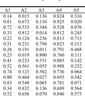
Table 1. Input sample
A1 A2 A3 A4 A5 0.14 0.015 0.136 0.824 0.316 0.81 0.673 0.134 0.925 0.020 0.72 0.533 0.344 0.528 0.076 0.33 0.812 0.014 0.812 0.245 0.22 0.124 0.236 0.813 0.713 0.51 0.231 0.794 0.823 0.313 0.26 0.191 0.011 0.791 0.468 0.23 0.019 0.800 0.760 0.111 0.41 0.233 0.531 0.885 0.142 0.52 0.561 0.055 0.988 0.252 0.74 0.123 0.562 0.736 0.064 0.80 0.464 0.027 0.693 0.542 0.83 0.548 0.065 0.781 0.071 0.34 0.832 0.136 0.689 0.564 0.52 0.656 0.070 0.846 0.573
Since SOM neural network is self-study without teachers, the network would cluster automatically. The elements of network input vector is five, and the scale is between [0, 1]. In order to achieve the best clustering effect, after many times of neural network training, the competing level of the network is designed as a 4×3 structure. Because the number of training frequency can affect the network clustering ability, here the set of training frequency is 100 times. By using the training function of MATLAB’s neural network toolbox to train the SOM neural network, with the increasing of the training steps, the mapping of neurons gradually become reasonable. After the network training finished, the weight should be set too. Afterwards, every time one weight is input, the network would cluster it automatically. The results of clustering are shown as Table 2:
Table 2.Output of clusters
sample 1 2 3 4 5 6 7 8 9 10 result 7 6 6 8 7 1 7 4 4 8 sample 11 12 13 14 15
result 2 3 6 5 5
Next modifying weight through training, the error should be set in advanced as 102, and the original weight is
0 1
a , to the training samples of Table 1, after 2 times modifying the new training samples can be gained. Because of the new training input samples’ weight is 5+1=6, then the input point of building BP neural network should be 6, the output point should be 4. Since each index is different from another, the distance between each vector’s number of levels is quite large in the original samples, in order to calculate easily and avoid part of neurons reaching their saturation state, the processing of samples’ input would be normalized. The network extension complement structure should be the one with single cryptic level, after many times experiments, the cryptic level’s neurons should be 12. The hyperbolic tangent of its transfer function should be:
22 1
1 x
f x
e
(10)
[image:7.595.207.406.646.690.2]In which, the smallest training frequency isN= 120, the smallest training time isT= 0.01, after updating the weight, the weight is aN , the actual training frequency is N, the change of the actual training time T can be seen in Table 3. When the weight is aN 0.0625, the training time is T 0.01, the training is over.
Table 3. Changes of weight, minimum of training times and minimum of training number
N
a 0 0.5 0.25 0.125 0.0625 0.03125
N 672 413 220 135 61 40
T 8.1 6.5 5.4 2.0 0.009 0.008
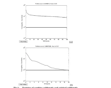
(a)
(b)
Fig 1: Training of combine arithmetic and original arithmetic
We can see from the Fig 1, when the training frequency is 100 in the original neural network, the error still has large distance with the error 102, and in the combine neural network can achieve the convergence after 20 times of
training.
After the simulation testing on the neural network that has been finished the training, the data of the testing samples is shown as the following Table 4:
Table 4. Emulate sample
[image:8.595.152.528.66.365.2]A1 A2 A3 A4 A5 0.24 0.556 0.043 0.785 0.422 0.53 0.022 0.234 0.672 0.034 0.91 0.134 0.172 0.964 0.087 0.36 0.082 0.061 0.561 0.328 0.54 0.253 0.072 0.987 0.899 0.72 0.634 0.763 0.943 0.266 0.13 0.196 0.566 0.674 0.305 0.22 0.314 0.345 0.655 0.275 0.41 0.020 0.781 0.861 0.306 0.54 0.654 0.095 0.975 0.124 0.93 0.782 0.034 0.658 0.032 0.37 0.034 0.342 0.605 0.067
Table 5. Result of emulation, corresponding fault and absolute error
[image:8.595.213.401.68.359.2] [image:8.595.178.436.635.759.2]The results, actual faults and errors of simulating the samples data of neural network in Table 4 that has been improved by using SOM method and LM method are shown as the following Table 5:
Based on the previous training and simulation results of neural network, we can see that the neural network that has been improved by using SOM and LM can converge speedily in the process of fault recognition, deduce its training frequency substantially, determine the fault type correctly, and the absolute error never reached 0.1, its accuracy is quite high.
CONCLUSION
This article studied on the computer network fault diagnosis, and imitating and simulating the computer network diagnosis by using SOM and LM. Based on the SOM neural network is a self-organized network with no teachers for competitive studying, the diagnosis of computer network fault does not require the particular recognition of the training samples’ actual fault types, and it has quite good clustering ability. SOM neural network and BP neural network can be united effectively by using the way of adding weights and improving BP neural network with the employment of LM algorithm. Through the practical examination, it proves that this method is accurate, efficient, which has very high theoretical meanings and application value.
REFERENCES
[1] Barlow B, Evans D,The Computer Journal,1997, vol. 6, no. 22, pp. 267-269.
[2] Chen T C, Han D J, Au F T K, et al,Neural Network Proceeding of the Internation Joint,2003, vol. 3, no. 4, pp. 1873~1878.
[3] Hangan M T, Menhaj M B,IEEE Transaction,1994.
[4] Hongjun liu, Huan liu,IEEE Trans on Knowledge and Data Eng,1996, vol. 34, no. 4, pp. 11-13.
[5] Jinggang Feng, Chengsheng Pan, Hang Li, Journal of shenyang industry institute, 2002, vol. 11, no. 4, pp.
234-236.
[6] Leary D P, Whiet R E,SIAMJ Alg Dis Meth,1985, vol. 6, no. 3, pp. 630-640.
[7] Lim\n Jin, Hongcai Zhan,Journal of northwestern polytechnical university,2004, vol. 22, no. 5, pp. 657-661. [8] M Riedmiler, H Braun, “A direct adaptive method for faster back propagation leaning: The RPROP algorithm,”
Proceedings of the IEEE International Conference on NeuralNetworks(ICNN),1993. [9] Sprecht D F,Neural Networks,1993, vol. 6, no. 4, pp. 1033-1034.
[10] T.Kohonen, “The “neural” phonetic type wirier,” Computer,1998, vol. 21, no. 3, pp. 11-22.; Xining Cui,
Quanyi Lv,Applied Mathematics and c computation,2006.
[11] Yongsheng Shi, Yunxue Song,Computer engineering,2004, vol. 30, no. 14, pp.125-127.