Multiobjective sensitivity analysis and optimization of distributed hydrologic model MOBIDIC

www.hydrol-earth-syst-sci.net/18/4101/2014/ doi:10.5194/hess-18-4101-2014

© Author(s) 2014. CC Attribution 3.0 License.

Multiobjective sensitivity analysis and optimization of distributed

hydrologic model MOBIDIC

J. Yang1, F. Castelli2, and Y. Chen1

1_{State Key Laboratory of Desert and Oasis Ecology, Xinjiang Institute of Ecology and Geography,} Chinese Academy of Sciences, Xinjiang, 830011, China

2_{Department of Civil and Environmental Engineering, University of Florence, Italy} Correspondence to: J. Yang ([email protected])

Received: 28 February 2014 – Published in Hydrol. Earth Syst. Sci. Discuss.: 26 March 2014 Revised: 27 August 2014 – Accepted: 8 September 2014 – Published: 15 October 2014

Abstract. Calibration of distributed hydrologic models usu-ally involves how to deal with the large number of dis-tributed parameters and optimization problems with mul-tiple but often conflicting objectives that arise in a natu-ral fashion. This study presents a multiobjective sensitiv-ity and optimization approach to handle these problems for the MOBIDIC (MOdello di Bilancio Idrologico DIstribuito e Continuo) distributed hydrologic model, which combines two sensitivity analysis techniques (the Morris method and the state-dependent parameter (SDP) method) with multi-objective optimization (MOO) approach ε-NSGAII (Non-dominated Sorting Genetic Algorithm-II). This approach was implemented to calibrate MOBIDIC with its application to the Davidson watershed, North Carolina, with three objec-tive functions, i.e., the standardized root mean square error (SRMSE) of logarithmic transformed discharge, the water balance index, and the mean absolute error of the logarithmic transformed flow duration curve, and its results were com-pared with those of a single objective optimization (SOO) with the traditional Nelder–Mead simplex algorithm used in MOBIDIC by taking the objective function as the Euclidean norm of these three objectives. Results show that (1) the two sensitivity analysis techniques are effective and efficient for determining the sensitive processes and insensitive parame-ters: surface runoff and evaporation are very sensitive pro-cesses to all three objective functions, while groundwater re-cession and soil hydraulic conductivity are not sensitive and were excluded in the optimization. (2) Both MOO and SOO lead to acceptable simulations; e.g., for MOO, the average Nash–Sutcliffe value is 0.75 in the calibration period and 0.70 in the validation period. (3) Evaporation and surface

runoff show similar importance for watershed water balance, while the contribution of baseflow can be ignored. (4) Com-pared to SOO, which was dependent on the initial starting location, MOO provides more insight into parameter sensi-tivity and the conflicting characteristics of these objective functions. Multiobjective sensitivity analysis and optimiza-tion provide an alternative way for future MOBIDIC model-ing.

1 Introduction

In the literature, to deal with the large number of dis-tributed model parameters, this is often done by aggregat-ing distributed parameters (e.g., Yang et al., 2007) or by screening out the unimportant parameters through a sensi-tivity analysis (e.g., Muleta and Nicklow, 2005; Yang, 2011). Sensitivity analysis can be used not only to screen out the most insensitive parameters, but also to study the system be-haviors identified by parameters and their interactions, qual-itatively or quantqual-itatively. However, most applications in en-vironmental modeling are based on a one-at-a-time (OAT) lo-cal sensitivity analysis, which is “predicated on assumptions of model linearity which appear unjustified in the cases re-viewed” (Saltelli and Annoni, 2010), or simple linear regres-sions, where a lot of uncertainties are not fairly accounted for. The use of global sensitivity analysis techniques is very cru-cial in distributed modeling. Only recently, global sensitivity analysis techniques and multiobjective sensitivity analysis started to appear in hydrologic modeling, and van Werkhoven et al. (2009) demonstrates how the calibration result responds to reduced parameter sets with different objectives and differ-ent metrics of parameter exclusion.

Although most hydrologic applications are based on the single objective calibration, model calibration with multiple and often conflicting objectives arises in a natural fashion in hydrologic modeling. This is not only due to the increasing availability of multivariable (e.g., flow, groundwater level, etc.) or multisite measurements, but also due to the intrin-sic different system responses (e.g., peaks and baseflow in the flow series). Instead of finding a single optimal solution in the single objective optimization (SOO), the task in the multiobjective optimization (MOO) is to identify a set of op-timal trade-off solutions (called a Pareto set) between con-flicting objectives. Although there are criticisms of MOO, such as that only one parameter set can be used for deci-sion making, recent studies (e.g., Kollat and Reed, 2007) have started to provide the answers. In hydrology, the tra-ditional method to solve multiobjective problems is to form a single objective, e.g., by giving different weights to these multiple objectives or by applying some transfer function. Over the past decade, several MOO algorithm approaches have been applied to the conceptual rainfall–runoff models (e.g., Yapo et al., 1998; Gupta et al., 1998, Madsen, 2000, Boyle et al., 2000; Vrugt et al., 2003; Liu and Sun, 2010), and are now increasingly applied to distributed hydrologic mod-els (e.g., Madsen, 2003; Bekele and Nicklow, 2007; Shafii and Smedt, 2009; MacLean et al., 2010). There are also some papers (Tang et al., 2006; Wöhling et al., 2008) to study their strengths comparatively with their application in hydrology. A good review of MOO applications in hydrological model-ing is given by Efstratiadis and Koutsoyiannis (2010). It is worth noting that the multiobjective calibration is different from statistical uncertainty analysis, which is based on the concept (or similar concept) of equifinality (see the discus-sions in Gupta et al., 1998, and Boyle et al., 2000).

Inf

Ad

Pc

Qg

Qd

R P

Wc

(Wcmax) _Wg

(Wgmax)

Et

(R+Qd)up

Groundwater storage H

River system Ws

α

CH

Ks

β γ

κ

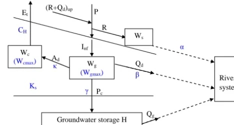
Figure 1. A schematic representation of MOBIDIC. Boxes denote

different water storages (gravitational storageWg, capillary storage Wc, groundwater storageH, surface storageWs, and the river sys-tem), solid arrows fluxes (evaporationEt, precipitationP, infiltra-tionInf, adsorptionAd, percolationPc, surface runoffR, interflow Qd, groundwater dischargeQg, and surface runoff and interflow from upper cells (R+Qd)up), dashed arrows different routings, and blue characters major model parameters.

This paper applies two sensitive analysis techniques (the Morris method and the state-dependent parameter (SDP) method) and ε-NSGAII (Non-dominated Sorting Genetic Algorithm-II) in the multiobjective sensitive analysis and calibration framework. This was implemented to calibrate the MOBIDIC (MOdello di Bilancio Idrologico DIstribuito e Continuo) distributed hydrological model with its application to the Davidson watershed, North Carolina. The purpose is to study the parameter sensitivity of the MOBIDIC hydrologic model and to explore the capability of MOO in calibrating the MOBIDIC model compared to the traditional SOO used in MOBIDIC applications.

This paper is structured as follows: Sect. 2 gives a de-scription of the MOBIDIC model; Sect. 3 introduces the approach in the multiobjective sensitivity analysis and op-timization; Sect. 4 gives a brief introduction of the study site, the model setup, objective selection, and the sensitivity and calibration procedures; in Sect. 5, the results are presented and discussed; and finally, the main results are summarized and conclusions are drawn in Sect. 6.

2 MOBIDIC hydrologic model

For each cell, water in the soil is simulated by dWg

dt =Inf−Sper−Qd−Sas

dWc

dt =Sas−Et,

(1)

where Wg (L) and Wc (L) are the water contents in the soil gravitational storage and capillary storage, respectively, andInf (LT−1),Sper(LT−1),Qd(LT−1),Et (LT−1) andSas (LT−1) are infiltration, percolation, interflow, evaporation, and adsorption from gravitational to capillary storage, which are modeled through the following equations:

Sper=γ·Wg Qd=β·Wg

Sas=κ·(1−Wc/Wc max), (2)

Inf=       

P+(Qd+Qh+Rd)up h

1−exp −Ks

P+(Qd+Qh+Rd)up

i

ifWg< Wgmax

0 otherwise

whereγ,βandκare the percolation coefficient (T−1), the in-terflow coefficient (T−1), and the soil adsorption coefficient (LT−1), respectively,P the precipitation (LT−1),QhandRd the Horton runoff and the Dunne runoff,Ksthe soil hydraulic conductivity (LT−1), andWgmax(L) andWcmax(L) the grav-itational and capillary storage capacities.

Once the surface runoff (Qh and Rd) and baseflow are calculated, three different methods can be used for river routing, i.e., the lag method, the linear reservoir method, and the Muskingum–Cunge method (Cunge, 1969). The Muskingum–Cunge method was used in this study.

MOBIDIC uses either a linear reservoir or the Dupuit ap-proximation to simulate the groundwater balance, which re-lates the groundwater change to the percolation, water loss in aquifers and baseflow. In this case study, the linear reservoir method was used.

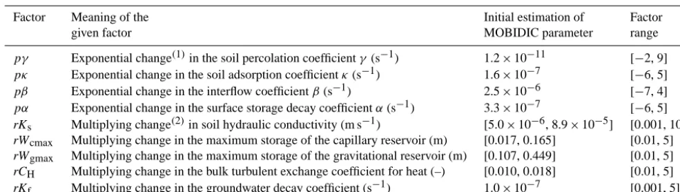
Although there are many distributed parameters in MO-BIDIC, these distributed parameters are normally calibrated through the “aggregate” factors (e.g., the multiplier for hy-draulic conductivity) based on their initial estimations, and hereafter we use the term “factor” (instead of “model pa-rameter”) when we conduct the sensitivity analysis and opti-mization, to avoid confusion with the term “model parame-ter” used in the model description. A factor can be a model parameter or a group of distributed model parameters with the same parameter name, and in this paper, it is a change to be applied to a group of model parameters. In MOBIDIC, nine factors (i.e., nine groups of parameters) normally need to be calibrated. These factors, their explanations, and their corresponding model parameters are listed in Table 1.

3 Methodology

The procedure applied here consists of two-step analyses, i.e., a multiobjective sensitivity analysis generally charac-terizing the basic hydrologic processes and singling out the most insensitive factors, and a multiobjective calibration aiming at trade-offs between different objective functions. 3.1 Sensitivity analysis techniques

Sensitivity analysis assesses how variations in model output can be apportioned, qualitatively or quantitatively, to differ-ent sources of variations, and how the given model depends upon the information fed into it (Saltelli et al., 2008). In the literature, a lot of sensitivity analysis methods are introduced and applied; e.g., Yang (2011) applied and compared five different sensitivity analysis methods. Here, we adopted an approach that combines two global sensitivity analysis tech-niques, i.e., the Morris method (Morris, 1991) and the SDP method (Ratto et al., 2007).

3.1.1 Morris method

The Morris method is based on a replicated and randomized one-factor-at-a-time design (Morris, 1991). For each factor

Xi, the Morris method uses two statistics,µi andσi, which

measure the degree of factor sensitivity and the degree of nonlinearity or factor interaction, respectively. The higherµi

is, the more important the factorXi is to the model output,

and the higherσi is, the more nonlinear the factorXi is to

the model output or more interactions with other factors (for details, refer to Morris, 1991, and Campolongo et al., 2007). The Morris method takesm∗(n+1) model runs to estimate these two sensitivity indices for each ofnfactors with sample sizem. The advantage is that it is efficient and effective for screening out insensitive factors. Normally mtakes values around 50, and according to Saltelli et al. (2008), the sensi-tivity measure (µi)is a good proxy for the total effect (i.e.,

STi in Eq. 4 below), which is a robust measure in sensitivity

analysis.

3.1.2 State-dependent parameter (SDP) method SDP (Ratto et al., 2007) is based on the ANOVA (ANal-ysis Of VAriance) functional decomposition, which appor-tions the model output uncertainty (100 %, as 1 in Eq. 3) to factors and different levels of their interactions:

1=X

i

Si+

X

i

X

j >i

Sij+. . .+S12..n (3)

whereSi is the main effect of factorXi representing the

av-erage output variance reduction that can be achieved when

Xi is fixed, andSij is the first-order interaction betweenXi

andXj, and so on. In ANOVA-based sensitivity analysis, the

total effect (STi) is frequently used, which stands for the

Table 1. Initial selected factors, initial estimation of the corresponding MOBIDIC parameter, and factor ranges.

Factor Meaning of the Initial estimation of Factor

given factor MOBIDIC parameter range

pγ Exponential change(1)in the soil percolation coefficientγ(s−1) 1.2×10−11 [−2, 9] pκ Exponential change in the soil adsorption coefficientκ(s−1) 1.6×10−7 [−6, 5] pβ Exponential change in the interflow coefficientβ(s−1) 2.5×10−6 [−7, 4] pα Exponential change in the surface storage decay coefficientα(s−1) 3.3×10−7 [−6, 5]

rKs Multiplying change(2)in soil hydraulic conductivity (m s−1) [5.0×10−6, 8.9×10−5] [0.001, 100]

rWcmax Multiplying change in the maximum storage of the capillary reservoir (m) [0.017, 0.165] [0.01, 5]

rWgmax Multiplying change in the maximum storage of the gravitational reservoir (m) [0.107, 0.449] [0.01, 5]

rCH Multiplying change in the bulk turbulent exchange coefficient for heat (–) [0.010, 0.018] [0.01, 5]

rKf Multiplying change in the groundwater decay coefficient (s−1) 1.0×10−7 [0.001, 5]

(1)_{Exponential change pX means the corresponding MOBIDIC parameterXwill be changed according toX=X}

0×exp(pX−1), whereX0is the initial estimation ofX. (2)_{Multiplying change rX means the corresponding MOBIDIC parameterXwill be changed according toX=X}

0×rX.

unknown.

STi =Si+

X

j6=i

Sij+. . .+S12...n (4)

The SDP method uses the emulation technique to approxi-mate lower-order sensitivity indices in Eq. (3) (e.g.,Si and

Sij in this study) by ignoring the higher-order sensitivity

in-dices, and we define SDi=Si+P j

Sij (referred to as the

“quasi total effect” later) as a surrogate for the total effect. The advantage is that it can precisely estimate lower-order sensitivity indices at a lower computational cost (normally 500 model runs, which is independent of the number of fac-tors). The disadvantage is that it cannot estimate higher-order sensitivity indices.

In practice, especially for over-parameterized cases, the Morris method is first suggested to screen out insensitive factors, and then the SDP method is applied to quantify the contributions of the sensitive factors and their interactions. In this study, as model parameters are aggregated into nine factors (as listed in Table 1), these two methods are applied individually. Then, the sensitivity of each factor and its sys-tem behaviour will be discussed, qualitatively by the Morris method, and quantitatively by the SDP method, and then the most insensitive factors will be screened out and excluded in the calibration.

In the context of multiobjective analysis, the sensitivity analysis applied includes (1) examination of the sensitivity of each factor to different objective functions, qualitatively or quantitatively, (2) singling out of the most sensitive fac-tors and study of the physical behaviors of the system, and (3) exclusion of the most insensitive factors, thereby simpli-fying the process of calibration. It is worth noting that the sensitivity analysis approach applied here is not a fully mul-tiobjective sensitivity analysis approach such as proposed by Rosolem et al. (2012, 2013), which applies sensitivity analy-sis to all objectives in an integrated way, and which is objec-tive. However, compared to the fully multiobjctive

sensitiv-ity analysis approach (as proposed in Rosolem et al., 2012), which easily requires over 10 000 model runs, our approach is very computationally efficient, as both the Morris method and the SDP method only need several hundred model runs, which is highly appreciable for physically based and dis-tributed hydrologic models.

3.2 Multiobjective calibration andε-NSGAII

In the literature of hydrologic modeling, most applications are single objective based, which aims at a single optimal solution. However, for example in flow calibration, there is always a case that for two solutions, one solution simulates the peaks better and simulates the baseflow poorly, while the other solution simulates the peaks poorly and simulates the baseflow better. These two solutions, called Pareto solutions, are incommensurable; i.e., better fitting of the peaks will lead to worse fitting of the baseflow, and vice versa. This belongs to the domain of MOO, aiming at finding a set of optimal solutions (Pareto solutions), instead of one single solution.

Generally, a MOO problem can be formulated as follows: min F (X)=(f1(X), f2(X), . . . , fi(X), . . . , fk(X))

s.t. G(X)=(g1(X), g2(X), . . . , gi(X), . . . , gl(X)),

(5) whereX is ann-dimensional vector and, in this study, rep-resents the model factors to be calibrated,fi(X)is theith

objective function, andgi(X)is theith constraint function.

In the literature, there are many algorithms available to obtain the Pareto solutions, e.g., NSGAII (Deb et al, 2002), SPEA2 (Strength Pareto Evolutionary Algorithm 2; Zitzler et al., 2001), MOSCEM-UA (Multiobjective Shuffled Complex Evolution Metropolis; Vrugt et al., 2003), and ε-NSGAII (Kollat and Reed, 2006), etc. In this study, we adopt ε -NSGAII, which is efficiency, reliability, and ease of use. Its strengths have been comparatively studied in Kollat and Reed (2006) and Tang et al. (2006).

The main characteristics ofε-NSGAII include the (i) selec-tion, crossover, and mutation processes as with other genetic algorithms by mimicking the process of natural evolution, (ii) an efficient non-domination sorting scheme, (iii) an elitist selection method that greatly aids in capturing Pareto fronts, (iv) εdominance archiving, (v) adaptive population sizing, and (vi) automatic termination to minimize the need for ex-tensive parameter calibration. For more details, refer to Kol-lat and Reed (2006). In this study, two changes were made to the original ε-NSGAII: (1) the initial population is gen-erated with the Sobol quasi-random sampling technique to improve the coverage of parameter space; and (2) the code is parallelized and interfaced with MOBIDIC to improve the computational speed.

As a comparison, a single objective function is defined as the 2-norm of the multiple objectivesF (X), which measures how close they are to the original point (theoretical optimum O):

sof= kF (X)k₂= v u u t

k

X

i=1

fi(X)2, (6)

and SOO was done with the classic Nelder–Mead algorithm (Nelder and Mead, 1965), which is already coded into the MOBIDIC package.

To analyze the Pareto solution and also to compare it with the solution from SOO, except for traditional methods, the “level diagram” proposed by Blasco et al. (2008) was also used. Compared to traditional methods, it can visualize high-dimensional Pareto fronts, and synchronizes the objective and factor diagrams. The procedure includes two steps. In the first step, the vector of objectives (kdimension) for each Pareto point is mapped to a real number (one dimension) ac-cording to the proximity to the theoretical optimum measured with a specific norm of objectives; and in the second step, these norm values are plotted against the corresponding val-ues of each objective or factor. 1-norm, 2-norm and∞-norm are suggested. For comparison with SOO, 2-norm was used.

4 Davidson watershed and objective selection 4.1 Davidson watershed

The Davidson watershed, located in the southwestern moun-tain area of North Carolina, drains an area of 105 km2above the Davidson River station near Brevard (see Fig. 2). The el-evation ranges from 645 to 1820 m above sea level. Based on the North American Land Data Assimilation System (NLDAS) climate data, the average annual precipitation is 1900 mm, and varies from 1400 mm to 2500 mm, and daily temperature changes from−19 to 26◦C. The average daily flow is about 3.68 m3s−1.

Data used in the MOBIDIC model include (i) a digi-tal elevation model (DEM), (ii) soil data, (iii) land cover

Figure 2. The location of the Davidson watershed, North Carolina,

with a DEM map, the river system (lines), and the watershed outlet (the triangle point).

data, (iv) climate data (precipitation, minimum and maxi-mum temperature, solar radiation, humidity and wind speed) and (v) flow data; a DEM of 9 m, land cover, SSURGO soil data, one station (the Davidson River near Brevard) of flow data from the US Geological Survey, and hourly NL-DAS climate data from the National Aeronautics and Space Administration (NASA). NLDAS integrates a large quantity of observation-based and model reanalysis data to drive of-fline (not coupled to the atmosphere) land-surface models (LSMs), and runs at 1/8 degree grid spacing over central North America, enabled by the Land Information System (LIS) (Kumar et al., 2006; Peters-Lidard et al., 2007).

A DEM is used to delineate the watershed and to estimate the topographic parameters and the river system, land cover for evaporation parameters, and soil data for soil parameters. Climate data are used to drive MOBIDIC, and flow data are used to calibrate the model and to assess model performance. The climate and flow data used in this study are from 1 Jan-uary 1996 to 30 September 2006. As NLDAS only has hourly temperature daily instead of the hourly minimum and max-imum temperatures needed by MOBIDIC, we compiled the hourly climate data to daily data and ran the model at a daily step. After MOBIDIC setup, the initial parameter values are listed in the third column of Table 1.

4.2 Objective function selection

After setting up MOBIDIC in the Davidson watershed, three objective functions were used in the multiobjective sensitiv-ity analysis and optimization:

1. Standardized root mean square error (SRMSE) between the logarithms of simulated and observed outflows:

SRMSE= q

1

N

PN

i=1(log Qobsi

₋

log Qsim_i

)2

q 1

N−1

PN

i=1(log Qobsi

−log¯Q)2

(7)

2. Water balance index (WBI), calculated as the mean ab-solute error between the simulated and observed flow accumulation curves:

WBI= 1 N

XN

i=1|Q

obs Ci −Q

sim

Ci | (8)

3. Mean absolute error between the logarithms of simu-lated and observed flow duration curves:

MARD= 1

100 XN

i=1|log

Qobs_Pi −logQsim_Pi | (9)

In Eqs. (7), (8) and (9),Qobs_i andQsim_i are observed and sim-ulated flow series at time stepi,N the data length, logQthe average of logarithmic transformed observed flows,Qobs_Ci and

Qsim_Ci theith observed and simulated accumulated flows, and

Qobs_Pi andQsim_Pi theith percentiles of observed and simulated flow duration curves.

SRMSE (Eq. 7), WBI (Eq. 8) and MARD (Eq. 9) are mea-sures of the closeness between simulated and observed flow series, water balance, and the closeness between simulated and observed flow frequencies, respectively. The smaller these measures are, the better the simulation is, and the min-ima are (0, 0, 0), meaning a perfect match between the simu-lation and the observation. It is worth noting that we use the logarithms of the flows instead of flows to avoid overfitting flow peaks (Boyle et al., 2000; Shafii and De Smedt, 2009), as flood forecasting is not our main focus, and for SRMSE, we have NS approximately equal to 1 SRMSE2whenN is large (e.g., > 100), where NS is the Nash–Sutcliffe coeffi-cient (Nash and Sutcliffe, 1970), which is widely used in hy-drologic modeling.

Accordingly, the single objective function here is the Eu-clidean norm (2-norm) of SRMSE, WBI and MARD:

sof=pSRMSE2+WBI2+MARD2 (10)

5 Result and discussion

5.1 Multiobjective sensitivity analysis

The Morris method and the SDP method were applied indi-vidually to the initially selected factors (in Table 1).

1 2 3 4 5 6

234567

SRMSE

μ

σ

0.0 0.2 0.4 0.6

0.2

0.3

0.4

0.5

0.6

WBI

μ

σ

0.5 1.5 2.5 3.5

1234

MARD

μ

σ

pγ pκ pβ pα

rKs

rWcmax

rWgmax

rCH

rKf

Figure 3. Multiobjective sensitivity analysis result based on the

Morris method (µis the sensitivity measure, andσ demonstrates the degree of nonlinearity or factor interaction).

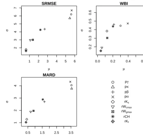
For the Morris method, its convergences for three objec-tive functions, monitored using the method proposed in Yang (2011), were achieved with around 700∼800 model simula-tions. Figure 3 gives the sensitivity results for objective func-tions SRMSE, WBI, and MARD, respectively. In each plot, the horizontal axis (µ) denotes the degree of factor sensi-tivity, and the vertical axis (σ )denotes the degree of factor nonlinearity or interaction with other factors.

For SRMSE, the most sensitive factors are group (pα,pγ, andpκ), followed bypβ and rCH, while other factors (es-pecially rKs and rKf)are not so sensitive. This applies to the degree of the factor nonlinearity or interaction. Factors in the same group have a similar effect on the studied objec-tive function. The sensitivities ofpα,pγ, andpκ indicate the importance of their corresponding processes (i.e., surface runoff, percolation, and adsorption, which is related to evap-otranspiration) for SRMSE, while interflow (pβ)is less im-portant, and other processes/characteristics (e.g., groundwa-ter flow and rKf)are not important.

For WBI, the dominating parameter is pκ, followed by

pα, pγ, pβ and rCH, while other factors (especially rKf and rWcmax)are not so sensitive. WBI measures the water balance between observed and simulated flow series, and it is reasonable that pκ, which controls the water supply for evaporation, is most sensitive, while other factors (pα,pγ,

pβ and rCH) are sensitive mainly through interaction with this factor, as indicated by the highσ of these factors.

pγ pκ pβ pα rKs rWcmax rWgmax rCH rKf

Si (R2_:58.7%)

Di (R2_:83.3%) SRMSE

sensitivity inde

x

0.00

0.10

0.20

0.30

pγ pκ pβ pα rKs rWcmax rWgmax rCH rKf

Si (R2_:38.4%)

Di (R2_:57.6%) WBI

sensitivity inde

x

0.0

0.1

0.2

0.3

0.4

pγ pκ pβ pα rKs rWcmax rWgmax rCH rKf

Si (R2:58.1%)

Di (R2:83.8%) MARD

sensitivity inde

x

0.00

0.10

0.20

0.30

Figure 4. Multiobjective sensitivity analysis result based on the

SDP method.

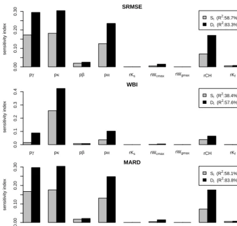
Figure 4 gives the sensitivity results based on the SDP method for SRMSE, WBI, and MARD, from top to bottom. In each plot, the grey and black bars areSi andSDi for each

factor.

For SRMSE, as indicated byR2in the legend, the main ef-fects (Si)contribute up to 58.7 % of the SRMSE uncertainty,

and quasi total effects (SDi)account for 83 % of the SRMSE

uncertainty, which is quite high, while another 17 % due to higher interactions are not explained. Based on SDi (black

bar), the most sensitive factors arepγ andpκ, followed by

pα and rCH, and thenpβ and rWcmax, while other factors are not sensitive. This result quantitatively corroborates the result obtained from the Morris method. The main effects (Si)ofpγ,pκ andpα are high (i.e., 0.17, 0.18 and 0.14),

which suggests that these factors should be determined first in model calibration, as they lead to the largest reduction in SRMSE uncertainty. For each factor, the difference between the black bar and the grey bar shows the first-order interac-tion with other factors. This interacinterac-tion is very strong inpγ,

pκ,pαand rCH, and is very weak in other factors.

For WBI, as indicated byR2in the legend, the total main effects (Si)contribute up to 38.4 % of the WBI uncertainty,

quasi total effects (SDi)only account for 57.6 % of the WBI

uncertainty, and around 40 % due to higher interactions are not explained and can not be ignored. However, by compar-ing the result with that from the Morris method (top-right corner in Fig. 3), we still can get some valuable results: the dominating sensitive factor is pκ, with SDi equal to 0.43

(which is the same as the Morris method), followed bypγ,

pα and rCH, while other factors are not sensitive; the main effect ofpκis as high as 0.27, and it should be fixed in order

Figure 5. The normalized factor sets associated with MOO (grey

lines) and the solution with SOO (dark line).

to get the maximum reduction in WBI uncertainty; the first interaction is high inpκ,pγ andpα, and is not obvious in other factors.

Similar to the Morris model results for SRMSE and MARD, the result of MARD is nearly the same as SRMSE. The similar result for SRMSE and MARD shows a similar characteristic relationship between the factors and the objec-tive function. This is explainable: a good simulation mea-sured by SRMSE will more likely result in a good measure of MARD, and vice versa.

As aforementioned, in the context of multiobjective sen-sitivity analysis, sensen-sitivity analysis excludes factors that are insensitive to all the objective functions considered. Based on the analysis above, the four most insensitive factors are rKs, rKf, rWcmaxand rWgmax. However, as shown in Fig. 4, rWcmax is more sensitive than the other three factors, and for the objective function WBI, as higher-order interactions are strongly based on SDP (i.e., explaining around 40 % of model uncertainty), evaporation is the most sensitive process to water balance (as indicated bypκ and rCH), and rWcmax is the only factor related to evaporation storage (Wc); there-fore, we only exclude rKf, rKsand rWgmaxfor calibration. 5.2 Multiobjective optimization

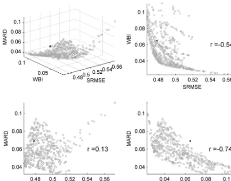
Figure 6. The Pareto solutions in the three-dimensional space (top

left), and the projections in the two-dimensional subspace (other plots), with MOO, and the black dot is the solution with SOO.

Figure 5 shows optimized non-dominant sets normalized within [0, 1], and the black line is for the factor set with SOO. It is encouraging that, except for rWcmax, factor ranges decreased a lot. This corroborates the conclusion in the sensi-tivity analysis:pγ,pκ,pβ,pα, and rCHare the most sensi-tive and identifiable factors in these three objecsensi-tive functions, while rWcmaxis less sensitive and less identifiable. Several scattered values ofpγ and dispersed rWgmaxshow that opti-mized factor sets are scattered in the response surface rather than concentrated in a continuous region, and the factor set with SOO is within the range of non-dominant sets.

Figure 6 shows Pareto solutions scattered in the three-dimensional space (top left), and projections in two-dimensional subspaces with the corresponding correlation coefficients (r)in the calibration period, with the black dot in each plot denoting the solution for SOO. Correlation coef-ficients are high and negative for SRMSE and WBI (−0.54), and for WBI and MARD (−0.74), and this indicates strong trade-off interactions along the Pareto surface; i.e., a bet-ter (lower) WBI will eventually result in a worse (higher) SRMSE, and vice versa. The correlation coefficient is low (0.13) between SRMSE and MARD, and is even lower when these two objectives approach their minimum regions (i.e., SRMSE < 0.53 and MARD < 0.09). This might indicate a poor choice of the objective function, as also shown by sim-ilar sensitivity results for these two objective functions in Sect. 5.1. Table 2 lists the statistics of these three objectives associated with Pareto sets and the result of SOO. For Pareto sets, in the calibration period, the average SRMSE is 0.49, ranging from 0.47 to 0.57, which corresponds to the average NS of 0.78, ranging from 0.67 to 0.78; the average WBI is 0.05, ranging from 0.02 to 0.11, and the average MEAD is 0.08, ranging from 0.03 to 0.11. In the validation period, the

average SRMSE is 0.54, ranging from 0.51 to 0.62, which corresponds to an average NS of 0.70, ranging from 0.61 to 0.74; the average WBI is 0.05, ranging from 0.04 to 0.09, and the average MEAD is 0.10, ranging from 0.08 to 0.13. For SOO, SRMSE, WBI and MEAD are 0.48, 0.06 and 0.07 for the calibration period, and 0.57, 0.06 and 0.10 for the validation, and accordingly the NS values are 0.77 and 0.67, respectively. According to Moriasi et al. (2007), which sug-gests NS > 0.75 and WBI < 10 % as excellent modeling of river discharge, all Pareto solutions with MOO and the so-lution with SOO are close to “excellent” for both the calibra-tion and validacalibra-tion periods.

To visualize Pareto sets better and to compare them with the result of SOO, the level diagrams are plotted in Fig. 7 by applying a Euclidean norm (2-norm) to evaluate the distance of each Pareto point to the ideal origin (0,0,0) (the ideal val-ues for all three normalized objectives are 0). In Fig. 7, the top three plots are for the three objectives, the rest are for optimized factors, and the black dot in each plot is the solu-tion for SOO. In the level diagrams, each objective and each factor of a point (corresponding to a Pareto solution) is repre-sented by the same 2-norm value for all the plots. Compared with MOO, obviously, SOO was trapped in the local optima, as seen in the top-left plot. Another SOO was done with its starting point close to the optimum of MOO, and now the optimum of SOO is very close to that of MOO, which means that optimization with the Nelder–Mead algorithm was de-pendent on the starting point. The 2-norm has a close linear relationship with SRMSE due to values of SRMSE being 5 to 10 times those of the other two objective functions, and it does not have such a relationship with the other two objec-tives. The scattering of objectives and factors makes it dif-ficult in decision making to select a single solution, because there is no clear trade-off solution (Blasco et al., 2008). How-ever, compared with SOO, the Pareto solutions from MOO can make decision making easy, as it can be converted with expert opinion or some utility function.

Table 2. Statistics of three objective functions associated with multiobjective optimization and single objective optimization.

Multiobjective optimization Single objective optimization

Calibration Validation Calibration Validation

Mean Min Max Mean Min Max

SRMSE 0.49 0.47 0.57 0.54 0.51 0.62 0.48 0.57 WBI 0.05 0.02 0.11 0.05 0.04 0.09 0.07 0.06 MARD 0.08 0.03 0.11 0.10 0.08 0.13 0.07 0.10

Figure 7. Two-norm level diagram representation of the Pareto sets with MOO, and the solution with SOO (black dot).

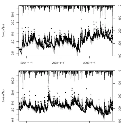
scale when computing objectives SRMSE and MARD. With SOO, the deviation from the observation is larger. Similar conclusions can be drawn from the time series simulations in Fig. 9, i.e., the wide ranges of low-flow periods, and under-estimation of flow peaks. Other than this, all simulations can generally mimic the observations.

Figure 8. Flow duration curve for observations (dotted line), and

simulated with MOO (grey) and SOO (solid line).

Figure 9. Observed flows (dotted) and simulated flows with MOO

(grey) and SOO (black line) for the calibration period (top) and val-idation period (bottom).

the solution with SOO, except for its ranges of soil satura-tion and groundwater (groundwater is very close to 0 mm). For fluxes with MOO, evaporation and surface runoff have more temporal variation than baseflow, and their magnitudes are larger than baseflow. This applies to fluxes with SOO, and its baseflow is close to 0. This can be confirmed by the De Finetti diagram in Fig. 11: with MOO, the average contri-butions of evaporation, surface runoff, and baseflow are 49.3, 46.1, and 4.8 %, respectively, while the contribution of base-flow is very insignificant, and the contribution of basebase-flow is almost 0 with SOO.

Figure 10. Time series of watershed average storages (soil water

storage expressed as soil saturation, and groundwater depth), and fluxes (evaporation, surface runoff, and baseflow) with MOO (grey) and SOO (black line). For SOO, the groundwater storage and base-flow are close to 0 and hardly seen.

Evaporation Baseflow

Surface runoff

0.2

0.8

0.2

0.4 _0.6

0.4

0.6

0.4

0.6

0.8

0.2

0.8

Figure 11. De Finetti diagram (ternary plot) of evaporation, surface

runoff, and baseflow with MOO (grey) and SOO (black star).

6 Conclusions

This study presents a multiobjective sensitivity and optimiza-tion approach to calibrating the MOBIDIC distributed hy-drologic model with its application in the Davidson water-shed for three objective functions (i.e., SRMSE, WBI and MARD). Results show that

1. The two sensitivity analysis techniques are effective and efficient in determining the sensitive processes and in-sensitive parameters: surface runoff and evaporation are very sensitive processes to all three objective functions, while groundwater recession and soil hydraulic conduc-tivity are not sensitive and were excluded from the opti-mization.

2. For SRMSE and MARD, all the factors have almost the same sensitivities, and a low correlation exists between these two objectives in the non-dominance of the Pareto set. This might indicate a poor choice of the objective function.

3. Both MOO and SOO achieved acceptable results for both the calibration period and the validation period in terms of objective functions and a visual match be-tween simulated and observed flows and flow duration curves. For example, with MOO, the average NS values are 0.75, ranging from 0.67 to 0.78 in the calibration period, and 0.70, ranging from 0.61 to 0.74 in the vali-dation period.

4. In the case study, evaporation and surface runoff show similar importance to the watershed water balance, while the contribution of baseflow can be ignored. 5. Comparing MOO with ε-NSGAII, the application of

SOO with the Neld–Mead algorithm was dependent on an initial starting point. Furthermore, the Pareto solu-tion provides a better understanding of these conflicting objectives and the relations between objectives and pa-rameters, and a better way for decision making.

Acknowledgements. The research was supported by the Thousand

Youth Talents plan (Xinjiang project) and the National Basic Research Program of China (973 Program: 2010CB951003). The data used in this study were acquired as part of the mission of NASA’s Earth Science Division and archived and distributed by the Goddard Earth Sciences (GES) Data and Information Services Center (DISC). The authors would like to thank Rafael Rosolem and the other two anonymous reviewers for valuable comments that substantially improved the manuscript.

Edited by: D. Solomatine

References

Bekele, E. G. and Nicklow, J. W.: Multi-objective automatic calibra-tion of SWAT using NSGA-II, J. Hydrol., 341, 165–176, 2007 Beven, K. and Binley, A.: The future of distributed models – model

calibration and uncertainty prediction, Hydrol. Process., 6, 279– 298, 1992.

Blasco, X., Herrero, J. M., Sanchis, J., and Martínez, M.: A new graphical visualization of n-dimensional Pareto front for decision-making in multiobjective optimization, Inform. Sci-ences, 178, 3908–3924, 2008

Boyle, D., Gupta, H., and Sorooshian, S.: Toward improved cali-bration of hydrologic models: combining the strengths of man-ual and automatic methods, Water Resour. Res., 36, 3663–3674, 2000.

Campo, L., Caparrini, F., and Castelli, F.: Use of multi-platform, multi-temporal remote-sensing data for calibration of a dis-tributed hydrological model: an application in the Arno basin, Italy, Hydrol. Process., 20, 2693–2712, 2006

Campolongo, F., Cariboni, J., and Saltelli, A.: An effective screen-ing design for sensitivity analysis of large models, Environ. Mod-ell. Softw., 22, 1509–1518, 2007.

Castelli, F., Menduni, G., Caparrini, F., and Mazzanti, B.: A dis-tributed package for sustainable water managment: a case study in the Arno basin, in: The Role of Hydrology in Water Resoures Management (Proceedings of a symposium held on the island of Capri, Italy, October 2008), IAHS Publ. 327, 2009.

Cunge, J. A.: On the subject of a flood propagation method (Musk-ingum method), J. Hydraul. Res., 7, 205–230, 1969.

Deb, K., Pratap, A., Agarwal, S., and Meyarivan, T.: A fast and eli-tist multiobjective genetic algorithm: NSGA-II, IEEE T. Evolut. Comput., 6, 182–97, 2002.

Efstratiadis, A. and Koutsoyiannis, D.: One decade of multi-objective calibration approaches in hydrological modelling: a re-view, Hydrol. Sci. J., 55, 58–78, 2010

Gupta, H., Sorooshian, S., and Yapo, P.: Toward improved cali-bration of hydrologic models: multiple and noncommensurable measures of information, Water Resour. Res., 34, 751–763, 1998. Kollat, J. B. and Reed, P. M.: Comparing state-of-the-art evolution-ary multiobjective algorithms for long-term groundwater moni-toring design, Adv. Water Resour., 29, 792–807, 2006.

Kollat, J. B. and Reed, P.: A framework for visually interactive decision-making and design using evolutionary multi-objective optimization (VIDEO), Environ. Model. Softw., 22, 1691–1704, 2007.

Kumar, S. V., Peters-Lidard, C. D., Tian, Y., Houser, P. R., Geiger, J., Olden, S., Lighty, L., Eastman, J. L., Doty, B., Dirmeyer, P., Adams, J., Mitchell, K., Wood, E. F., and Sheffield, J.: Land information system – an interoperable frame-work for high resolution land surface modeling, Environ. Modell. Softw., 21, 1402–1415, 2006.

Liu, Y. and Sun, F.: Sensitivity analysis and automatic calibration of a rainfall–runoff model using multiobjectives, Ecol. Inform., 5, 304–310, 2010.

Madsen, H.: Automatic calibration of a conceptual rainfall–runoff model using multiple objectives, J. Hydrol., 235, 276–88, 2000. Madsen, H.: Parameter estimation in distributed hydrological

catch-ment modelling using automatic calibration with multiple objec-tives, Adv. Water Resour., 26, 205–216, 2003.

Moriasi, D., Arnold, J., Van Liew, M., Bingner, R., Harmel, R., and Veith, T.: Model evaluation guidelines for systematic quantifica-tion of accuracy in watershed simulaquantifica-tions, T. ASABE, 50, 885– 900, 2007.

Morris, M. D.: Factorial sampling plans for preliminary computa-tional experiments, Technometrics, 33, 161–174, 1991. Muleta, M. K. and Nicklow, J. W.: Sensitivity and uncertainty

analy-sis coupled with automatic calibration for a distributed watershed model, J. Hydrol., 306, 127–145, 2005.

Nash, J. E. and Sutcliffe, J. V.: River flow forecasting through con-ceptual models part I – A discussion of principles, J. Hydrol., 10, 282–290, 1970.

Nelder, J. A. and Mead, R.: A simplex method for function mini-mization, Comput. J., 7, 308–313, 1965.

Peters-Lidard, C. D., Houser, P. R., Tian, Y., Kumar, S. V., Geiger, J., Olden, S., Lighty, L., Doty, B., Dirmeyer, P., Adams, J., Mitchell, K., Wood, E. F., and Sheffield, J.: High-performance Earth system modeling with NASA/GSFC’s Land Information System, Innov. Sys., and Soft. Eng., 3, 157–165, 2007.

Ratto, M., Pagano, A., and Young, P.: State dependent parameter meta-modelling and sensitivity analysis, Comput. Phys. Com-mun., 177, 863–876, 2007.

Refsgaard, J. C. and Storm, B.: MIKE SHE, in: Computer Models in Watershed Hydrology, edited by Singh, V. J., Water Resour. Publications, Rome, Italy, 809–846, 1995.

Rosolem, R., Gupta, H. V., Shuttleworth, W. J., Zeng, X., and Gonçalves, L. G. G.: A fully multiple-criteria implementation of the Sobol’ method for parameter sensitivity analysis, J. Geophys. Res. Atmos., 117, D07103, doi:10.1029/2011JD016355, 2012. Rosolem, R., Gupta, H. V., Shuttleworth, W. J., Gonçalves, L. G.

G., and Zeng, X.: Towards a comprehensive approach to parame-ter estimation in land surface parameparame-terization schemes, Hydrol. Process., 27, 2075–2097, 2013.

Saltelli, A. and Annoni, P.: How to avoid a perfunctory sensitivity analysis, Environ. Modell. Softw., 25, 1508–1517, 2010. Saltelli, A., Ratto, M., Andres, T., Campolongo, F., Cariboni, J.,

Gatelli, D., Saisana, M., and Tarantola, S.: Global Sensitivity Analysis, The Primer, Wiley and Sons, Chichester, UK, 2008. Shafii, M. and De Smedt, F.: Multi-objective calibration of a

dis-tributed hydrological model (WetSpa) using a genetic algorithm, Hydrol. Earth Syst. Sci., 13, 2137–2149, doi:10.5194/hess-13-2137-2009, 2009.

Tang, Y., Reed, P., and Wagener, T.: How effective and effi-cient are multiobjective evolutionary algorithms at hydrologic model calibration?, Hydrol. Earth Syst. Sci., 10, 289–307, doi:10.5194/hess-10-289-2006, 2006.

Van Werkhoven, K., Wagener, T., Reed, P., and Tang, Y.: Sensitivity-guided reduction of parametric dimensionality for multi-objective calibration of watershed models, Adv. Water Re-sour., 32, 1154–1169, 2009.

Vrugt, J., Gupta, H. V., Bastidas, L. A., Bouten, W., and Sorooshian, S.: Effective and efficient algorithm for multiobjective opti-mization of hydrologic models, Water Resour. Res., 39, 1214, doi:1210.1029/2002WR001746, 2003.

Wöhling, T., Barkle, G. F., and Vrugt, J. A.: Comparison of three multiobjective optimization algorithms for inverse modeling of vadose zone hydraulic properties, Soil Sci. Soc. Am. J., 72, 305– 319, 2008

Yang, J., Reichert, P., Abbaspour, K. C., and Yang, H.: Hydrolog-ical modelling of the Chaohe Basin in China: statistHydrolog-ical model formulation and Bayesian inference, J. Hydrol., 340, 167–182, 2007.

Yang, J.: Convergence and uncertainty analyses in Monte-Carlo based sensitivity analysis, Environ. Model. Softw., 26, 444–457, 2011.