The Budyko and complementary relationships in an idealized model of large scale land–atmosphere coupling

www.hydrol-earth-syst-sci.net/19/2119/2015/ doi:10.5194/hess-19-2119-2015

© Author(s) 2015. CC Attribution 3.0 License.

The Budyko and complementary relationships in an idealized model

of large-scale land–atmosphere coupling

B. R. Lintner1, P. Gentine2, K. L. Findell3, and G. D. Salvucci4

1_{Department of Environmental Sciences, Rutgers, The State University of New Jersey, New Brunswick, NJ, USA} 2_{Department of Earth and Environmental Engineering and Earth Institute, Columbia University, New York, NY, USA} 3_{Geophysical Fluid Dynamics Laboratory, Princeton, NJ, USA}

4_{Department of Earth and Environment, Boston University, Boston, MA, USA} Correspondence to: B. R. Lintner ([email protected])

Received: 15 May 2014 – Published in Hydrol. Earth Syst. Sci. Discuss.: 7 August 2014 Revised: 18 February 2015 – Accepted: 23 February 2015 – Published: 4 May 2015

Abstract. Two well-known relationships in hydrology and hydrometeorology, the Budyko and complementary relation-ships, are examined within an idealized prototype represent-ing the physics of large-scale land–atmosphere couplrepresent-ing de-veloped in prior work. These relationships are shown to hold on long (climatologic) timescales because of the tight cou-pling that exists between precipitation, atmospheric radia-tion, moisture convergence and advection. The slope of the CR is shown to be dependent on the Clausius–Clapeyron relationship between saturation-specific humidity and tem-perature, with important implications for the continental hy-drologic cycle in a warming climate; e.g., one consequence of this dependence is that the CR may be expected to be-come more asymmetric with warming, as higher values of the slope imply a larger change in potential evaporation for a given change in evapotranspiration. In addition, the trans-parent physics of the prototype permits diagnosis of the sen-sitivity of the Budyko and complementary relationships to various atmospheric and land surface processes. Here, the impacts of anthropogenic influences, including large-scale ir-rigation and global warming, are assessed.

1 Introduction

Observations of the annual terrestrial surface water balance demonstrate a tight and relatively simple functional depen-dence of evapotranspiration on the atmospheric water sup-ply (precipitation) and demand (potential evaporation) at the surface (Budyko, 1961; Porporato et al., 2004; Roderick and

Farquahr, 2011; Williams et al., 2012; Zanardo et al., 2012). Such observations have stimulated development of simplified analytical formulations of the annual water balance (Budyko, 1961; Lettau, 1969; Eagleson, 1978a, b, c; Fu, 1981; Milly, 1994; Porporato et al., 2004; Harman et al., 2011; Siva-palan et al., 2011). Budyko (1961, 1974) developed ar-guably the most well-known approach for characterizing catchment-scale hydrologic balances on long (decadal and greater) timescales. By hypothesizing limitations on land sur-face evapotranspiration imposed by the availability of water and energy, Budyko introduced a relationship of the form

E P =B

_E

p

P

, (1)

whereE,P, andEpare evapotranspiration, potential evapo-transpiration, and precipitation, respectively. The ratioEp/P is commonly known as the dryness or aridity index (φ), and hereafter we denote the ratio E/P as B(φ), i.e., the Budyko curve. Empirical forms ofB(φ)have been obtained by fitting to observedE,P, andEp withE typically esti-mated as the residual of precipitation and basin-scale stream-flow (Budyko, 1961, 1974).B (φ) appears to be rather sta-ble across different regions and hydroclimatic environments (Potter et al., 2005; Yang et al., 2007; Gentine et al., 2012).

sim-plified models of the surface and groundwater moisture re-sponse to precipitation forced by Ep to investigate the ro-bustness of the Budyko curve in different catchments. Milly (1994) and Porporato et al. (2004), in particular, investigated the response of the annual water balance to changes in the characteristics of potential evaporation and precipitation in-tensity and frequency, yielding new insights into the sensi-tivity of the annual water balance to changes in surface en-ergy and water forcing, all other factors, e.g., vegetation char-acteristics, soil, and topography, remaining constant. How-ever, apart from a few studies investigating the catchment co-evolution and adaptation of vegetation to the water and energy forcing (Troch et al., 2009; Sivapalan et al., 2011; Gentine et al., 2012), a direct explanation of the stability and widespread applicability of the Budyko relationship across a range of conditions remains elusive.

In the Budyko framework, as in most hydrologic mod-els, Ep is prescribed as a forcing, which is thought to be independent of the surface. Nonetheless, E and Ep have been hypothesized to be inversely related to one another (Bouchet, 1963; Morton, 1983; Brutsaert and Stricker, 1979; Hobbins et al., 2001) on daily to annual timescales. In fact, the coupling between E and Ep provides the basis for a foundational relationship in hydrometeorology: the comple-mentary relationship, first introduced by Bouchet (1963) and Morton (1983). Mathematically, the complementary relation-ship (CR) can be expressed as

Ep+bE=(1+b)Ewet. (2)

In Eq. (2),Epis potential evaporation andEwetis the energy-limited, wet surface equilibrium evapotranspiration. Bouchet (1963) assumed a value of 1 for the scale factorb, while Pet-tijohn and Salvucci (2009), hereafter PS09, report values in the range 3–6 based on numerical simulations of an evapo-ration pan in a drying environment. SinceEpcannot directly be measured, pan evaporation has often been used in lieu of potential evaporation using a pan correction factor (Bosman, 1987; Roderick and Farquahr, 2004; van Heerwaarden et al., 2010). Kahler and Brutsaert (2006) assumed that use of pan measurements in Eq. (2) may account forb >1 because a pan transmits heat, resulting in warmer water inside the pan relative to a larger free water body (e.g., lake) under similar ambient conditions.

Although several studies (Zhang et al., 2004; Ramirez et al., 2005; Szilagyi and Jozsa, 2009) have discussed possible links between the CR and the Budyko curve, to date a the-oretical framework encompassing either or both of these re-lationships is still absent. Milly (1994) underscores the lack of physical understanding for why the Budyko curve devi-ates from its water- and energy-limited asymptotes, while Ramirez et al. (2005) suggest that, apart from heuristic ar-guments or under restrictive conditions, no general proof of the CR is available. Moreover, questions remain about the applicability and validity of the Budyko and complemen-tary relationships across different spatial and temporal scales.

Here, we note that observational data confirm the CR holds on daily to annual timescales (Bouchet, 1963; Kahler and Brutsaert, 2006) and across local to regional spatial scales (Granger, 1989; Szilagyi, 2001; Crago and Crowley, 2005; PS09; van Heerwaarden et al., 2010), which is usually under-stood in terms of the diurnal-scale interactions of the bound-ary layer with the surface, although questions have been raised about some of the assumptions inherent in these ap-proaches. Indeed, as PS09 note, some explanations for the CR have relied on contradictory assumptions. For exam-ple, the derivation of Szilagyi (2001) assumes that asE de-creases, the surface temperature of the evaporation pan re-mains constant while the overlying near surface-specific hu-midity decreases, increasing the vapor deficit and thus the evaporation rate over the pan. By contrast, in Granger (1989), surface temperature is assumed to increase while specific hu-midity remains constant, thus also increasing the huhu-midity gradient and pan evaporation rate. L’homme and Guilioni (2006) have questioned the physical validity and applicabil-ity of these assumptions.

In the present study, we make use of a semi-analytic, ideal-ized prototype of large-scale land–atmosphere coupling de-veloped in prior work (Lintner et al., 2013) to derive the Budyko and complementary relationships. Our approach dif-fers from prior analyses in that (i) it is implicitly large-scale and relevant on climatic timescales, and (ii) convergence, ad-vection, precipitation and atmospheric radiation are treated implicitly rather than as exogenous forcing. The latter ren-ders the atmospheric and surface moisture interactive and tightly coupled vertically but also horizontally – through the (nonlocal) effects of moisture advection and convergence. Several studies have pointed out that such tight coupling be-tween radiation, larger-scale circulation and the local surface energy budget is key to understanding locally observed land– atmosphere interactions (Betts et al., 1996, 2003, 2014; Betts and Viterbo, 2005; Betts, 2007). The analytic simplicity of the idealized prototype facilitates straightforward diagnosis of factors influencing the large-scale coupling, as highlighted in Lintner et al. (2013).

A key motivation for this study is consideration of how the continental hydrologic cycle, and more precisely how the be-havior reflected in the Budyko curve and CR, may respond to anthropogenic influences. Indeed, the projected response of the terrestrial hydrologic cycle to various climate change mechanisms in models remains subject to large uncertainties (Sherwood and Fu, 2014). Emergent behaviors such as the Budyko and complementary relationships may provide use-ful constraints on such uncertainties. For example, Brutsaert and Parlange (1998) have suggested that the CR may explain the apparent paradox between observed downward trends in pan evapotranspiration over the late twentieth century, and anticipated increases in evaporation resulting from a more intense hydrologic cycle in a warming atmosphere.

(Sect. 2), we analyze the generalized Budyko and comple-mentary relationships within our prototype (Sect. 3) and con-sider the physical parameters and processes impacting these relationships (Sect. 4). Here, we are interested in examin-ing the behavior across a range of hydroclimatic states; in what follows, we use the term “prototype transect” to refer to this range. This may be viewed as representing either a spatial sampling of states across a climatological gradient in soil moisture at a fixed point in time or a temporal sampling (as under the seasonal evolution) at a fixed point in space. In Sect. 5, we examine how anthropogenic influences such as global warming and large-scale irrigation affect these re-lationships.

2 Overview of the idealized land–atmosphere coupling prototype

In prior work (Lintner et al., 2013), we developed a semi-analytic prototype for land–atmosphere coupling. This pro-totype describes the coupling at spatial scales for which both local (evapotranspiration) and nonlocal processes (horizon-tal moisture advection and convergence) may be important to the water cycle budget. We consider steady-state conditions, corresponding to the climatological state of the hydrologic cycle. Although the steady-state assumption clearly limits the applicability of our model in the presence of important time-dependent processes operating in the climate system, we again note that the CR has been observed to hold across a range of timescales. Similarly, Budyko curves have been estimated from yearly mean observations (Budyko, 1974; Gentine et al., 2012).

The atmospheric component of this prototype is based on vertically integrated tropospheric temperature and moisture equations from the Quasi-equilibrium Tropical Circulation Model (QTCM; Neelin and Zeng, 2000; Zeng et al., 2000), an intermediate level complexity model for the tropical at-mosphere:

−Ms∇_H·v+P+Rnet+H=0, (3) Mq∇_H·v−P+E−vq· ∇Hq=0, (4) where∇_His the horizontal gradient operator;Rnetis the net column (top of the atmosphere minus surface) radiative heat-ing; Ms and Mq are the dry static stability and moisture strat-ification and∇_H·v is signed positive for low-level conver-gence; andvqis the vertically averaged horizontal wind vec-tor weighted by the moisture vertical structure assumed in QTCM1. (Note that baseline values for parameters such as Ms and Mq are given in Lintner et al., 2013, and references therein. Table 1 summarizes the parameter values most rele-vant to the present study.) The termP in Eqs. (3) and (4) rep-resents the net convective (condensational) heating and dry-ing, respectively; the negative sign in Eq. (4) indicates that precipitation is a net sink of vertically averaged tropospheric

moisture. For the temperature Eq. (3), we have neglected hor-izontal temperature gradients following the weak tempera-ture gradient assumption (Sobel and Bretherton, 2000; Sobel et al., 2001). Note that all terms appearing in Eqs. (3) and (4) are implicitly scaled to units of mm day−1by absorbing con-stants such as (specific) heat capacity, latent heat of fusion, and column mass per unit area1p/g, where1pis the tropo-spheric pressure depth.

A steady balanced surface energy flux constraint, in which the annual-mean ground surface heat flux is neglected, reads

Rsurf−E−H=0, (5)

where the net surface radiative heating,Rsurf, is signed posi-tive downward.

In Lintner et al. (2013), we consider tropospheric temper-ature (T) as prescribed and solve the system of Eqs. (3)–(5) forq,∇_H·v, and surface temperatureTsfor prescribed large-scale advection. A closed-form, self-consistent solution can be obtained by invoking the steady-state soil moisture bud-get:

P−E−Qrunoff=0, (6)

whereQrunoffis the net runoff. For analytic simplicity, we as-sume a simple bucket model, with an evaporative efficiency,

β= E

Ep, for which we assume a simple linear relationship β=w(Porporato et al., 2001, 2004), wherewis the dimen-sionless soil moisture (actual soil moisture normalized by a holding capacity).Qrunoff is represented as the precipita-tion rate times a power law of soil moisture,Qrunoff=P wη (Kirchner, 2009). The baseline power law scaling exponent isη=4, the value used in Lintner et al. (2013). The suitabil-ity of invoking a single moisture storage variable to repre-sent both basin-scale evaporative efficiency and runoff has recently been demonstrated at nine watersheds containing Ameriflux eddy covariance measurements of evaporation and gauged streamflow (Tuttle and Salvucci, 2012).

For analytic simplicity, we consider linearized radiative and surface turbulent fluxes of the form

H=H0+εH(Tss−a1sT )

E=β[Ep0+εH(γ Ts−b1sq) (7)

Rx=Rx0+ε_TR_sxTs+εR_TxT+εRqxq+cxP

Quantities with subscript “0” denote the values about which the fluxes are linearized, with coefficientsεrepresenting the linear sensitivity of fluxes toT,q, andTs. The scale factors

a1sandb1srelate vertically averaged temperature and mois-ture to near-surface values appropriate for computation of surface bulk turbulent fluxes. The coefficientγ=dq∗

Table 1. Parameter definitions and values in the baseline land–atmosphere coupling prototype.

Parameter Definition Value

a1s Weighting factor for surface temperature 0.30

α Priestley–Taylor coefficient 1.26

b1s Weighting factor for surface moisture 1.15

b Complementary relationship scale factor –

csurf Surface cloud longwave forcing coefficient 0.18

γ Dimensionless slope of Clausius–Clapeyron relationship 3.5

εH Linearized surface turbulent flux scaling coefficient 42 mm day−1K−1

η Runoff power law scaling exponent 4

τc Convective adjustment timescale 2 h

andx=surf), and the coefficientscxare cloud-radiative forc-ing sensitivities, with cloud-radiative fluxes assumed to be linearly proportional to the precipitation rate. Precipitation (convective heating in Eq. 3 or convective drying in Eq. 4) is formulated in terms of a Betts and Miller (1986) type relax-ation scheme:

P =maxεc(q−qc(T )) ,0. (8)

Here,qc(T )is a temperature-dependent moisture threshold andεcis the convective adjustment rate coefficient (inversely related to the timescale for convective adjustmentτc).

3 Overview of the baseline relationships 3.1 Complementary relationship

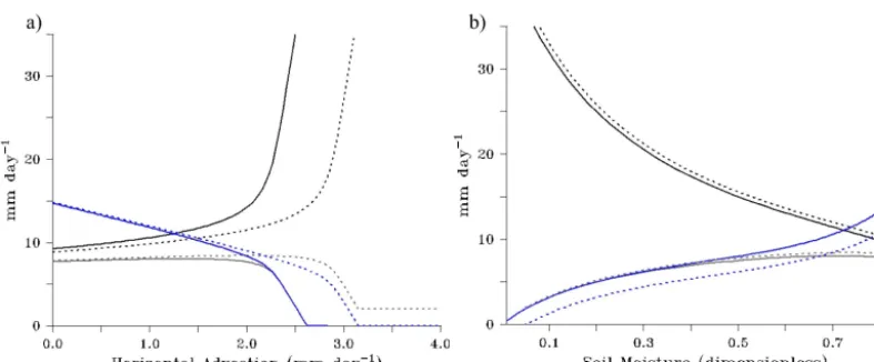
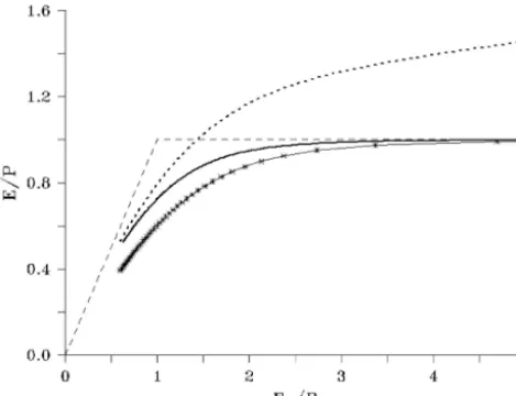
Figure 1a illustrates the functional relationships between soil moisture andE,P, andEpof the prototype. The general re-sponse ofE andEp with increasing soil moisture, namely Ep decreasing and E (generally) increasing, is consistent with the CR (Eq. 2). Eprelates towthrough the deficit be-tween ambient and saturation-specific humidity at the sur-face (Lintner et al., 2013): the deficit decreases with increas-ing soil moisture since q increases and Ts decreases. Fig-ure 2 depicts the results of the prototype against EandEp observations from the Little Washita River basin near Chick-asha, Oklahoma (see Kahler and Brutsaert, 2006, for a full description of the data set). Here,Epwas obtained directly from pan evaporation measurements with a correction factor and Ewas measured using the Bowen ratio (EBBR) tech-nique. E and Ep are presented in dimensionless units by dividing by the Priestly and Taylor (1972) evaporation, i.e.,

Ewet=α₁+γγRsurf, whereαis a correction factor with an es-timated value of∼1.26. The CR from the prototype shows a qualitative, and arguably even quantitative, correspondence to both observational data sets. Of course, we should point out that the prototype was not explicitly tuned to represent the hydroclimate of these locations, and as such, any quan-titative correspondence may be coincidental. Moreover, the

scatter inherent in the observations would permit a range of plausible complementary relationships.

A slight decrease inEis observed forw&0.7 (see the gray curve in Fig. 1a). To our knowledge, such a decrease has not been previously investigated, even though it appears in in situ measurements (Kahler and Brutsaert, 2006; PS09), as evi-dent in Fig. 2. The decrease in bothEandEparises from the monotonic decrease inEp

_∂E

p ∂w <0

at large soil moisture, as pointed out by Lintner et al. (2013). Indeed, in the proto-type, increasing soil moisture is a consequence of increasing precipitation, with the latter progressively balanced by higher moisture convergence (cf. Fig. 3 of Lintner et al., 2013). In-creasing moisture convergence is associated with inIn-creasing (low-level) humidity, which reduces the surface vapor pres-sure deficit, thereby reducingEp. Overall, the moisture bal-ance at large soil moisture values implies a greater role for nonlocal processes. On the other hand, at very low soil mois-ture values, meanP is mostly balanced by E, resulting in a tight link among E, Ep, and w. This explains the suc-cess of local coupled land-boundary layer models (Bouchet, 1963; van Heerwaarden et al., 2010) in representing the drier regime of the CR.

In prior studies of the CR, a quantityEwetwas introduced to denote the point of convergence ofEandEpunder unlim-ited soil moisture (saturated surface) conditions, i.e., at high soil moisture values (see Eq. 2). Conventionally,Ewetis as-sumed to represent equilibriumE from a saturated surface when advection is minimal and is usually computed empir-ically following Priestly and Taylor (1972). While the pro-totypeEp does indeed converge towardEas soil moisture increases, there is in fact no unique value ofEwetbecause of the declineEat high soil moisture.

Figure 1. Complementary relationship in the baseline configuration. (a) Potential evapotranspiration (Ep; black), evapotranspiration (E;

gray), and precipitation (P; blue) as functions of soil moisture (w). (b)Epvs.E(black) and the 1:1 line (gray). Also shown is the best fit

linear regression of theEptoErelationship (squares).

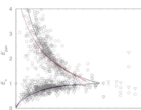
Figure 2. Baseline complementary relationship compared to Kahler

and Brutsaert’s observational data from the Little Washita River basin in Oklahoma, USA (cf. Fig. 5 in Kahler and Brutsaert, 2006). Symbols shown correspond to two different normalizations of the observations and gray lines to best fits through these points. The values along the abscissa,EMI, correspond to the ratio of actual to

pan evaporation in Kahler and Brutsaert (2006) and are identical to soil moisture in the prototype. PrototypeEpandE(red and purple

curves, respective) have been normalized with respect to the value ofEwetcorresponding to the maximum value ofEalong the

tran-sect.

This value ofbis quantitatively consistent with the estimates of Kahler and Brutsaert (2006), Szilagyi (2007), and PS09, and, unlike the original treatment of Bouchet (with b=1), implies a strongly asymmetric CR. The implied value ofbis close toγ, the dimensionless slope of the saturation-specific humidity curve, which is 3.5 in the baseline configuration; in fact, as we show in the parameter sensitivity analyses in Sect. 4.1,bvaries predominantly withγ, which is consistent with the theoretical arguments presented in Granger (1989).

We can, in fact, derive an analytic expression for the CR for our land–atmosphere coupling prototype. We begin by subtracting γ H from Ep and invoke the zero surface flux constraint to yield

Ep−γ H=Ep+γ E−γ Rs. (9)

Then, using the bulk formulae expressions forEpandH, the left-hand side of Eq. (9) can be expanded as

Ep−γ H=H(a1sγ T −b1sq) . (10)

Since precipitation rateP =c(q−qc(T )),q can be elimi-nated in favor ofP, which upon rearranging the terms gives

Ep+γ E=γ Rs− b1sH

c

P+f (T ). (11)

In Eq. (11),f (T )=H(1+γ )−1a1sγ T−b1sqc(T )is just a function of the (prescribed) tropospheric temperature, and is thus constant over the prototype transect.

Comparing Eq. (11) with Eq. (2), we find

b=γ (12)

and

Ewet=(1+γ )−1

γ Rs+f (T )− b1sH

c P

. (13)

As discussed above, in prior work,Ewet was defined using the relationship of Priestley and Taylor (1972). The term

(1+γ )−1γ Rsin Eq. (13) corresponds to the Priestley–Taylor formulation but with a coefficient of 1 in lieu ofα. It is worth noting that Kahler and Brutsaert’s in situ observations im-ply a Priestley–Taylor coefficient in the range of 0.89–1.13, which is in line with the value of 1 for the coefficient of

Ewetsuggested by Eq. (13). The remaining terms inEwetare not explicitly represented in the Priestley–Taylor relationship

through variation of the Priestley–Taylor coefficient. How-ever, we note that the dependence of Eq. (13) on precipitation implies a negative feedback of P on the Ewet, since higher tropospheric moisture is associated with higher precipitation, thereby decreasing vapor pressure deficit at the surface and suppressingEwet. This is consistent with the decrease inE at high soil moisture evident in Fig. 1a.

It is obvious thatEwetas defined by Eq. (13) is not constant across the prototype transect, as it depends on surface radia-tive heating and precipitation. (In a more general model, vari-ations in tropospheric temperature across the transect would also impact the value ofEwet.) Again, we point out that the Priestley–Taylor relationship only shows an explicit depen-dence on radiation (and the Clausius–Clapeyron slope). In addition to the negative feedback of precipitation on Ewet through the vapor deficit,Rsurfitself also decreases asP in-creases, owing to the negative cloud-radiative forcing asso-ciated with deep convective clouds (see Lintner et al., 2013). Related to the non-constancy ofEwet, we also note that the value of b differs slightly from the value inferred from di-rectly fitting to the linear portion of theEp vs.E curve in Fig. 1b.

3.2 Budyko curve

Within our prototype, the steady-state soil moisture Eq. (6) can be recast as

B (φ)=1−Qrunoff/P. (14)

For the simple case of a land surface bucket model with a runoff power law scaling exponent ofη=2, and noting that soil moisture can be expressed as w=β (w)= E

Ep = B(φ)

φ , Eq. (14) reduces to a quadratic equation in B (φ), with an analytic solution in terms ofφexpressed as

B (φ)=φ 2

2

s

1+ 4

φ2−1

!

. (15)

Figure 3 illustrates the Budyko curves for the baseline con-figuration of the prototype (η=4) and the analytic solution forη=2, with Budyko’s well-known empirical formulation

B (φ)=

q

φtanh φ−1

1−e−φ

for comparison. Also de-picted are the energy- and water-limited asymptotes. For the baseline configuration, B (φ) at intermediate values of the aridity index lies above the empirical Budyko fit, while the

η=2 curve lies below. Variation in the shape ofB (φ)with increasing values of ηis consistent with decreasing runoff for a given value of precipitation, which in turn necessitates shifting the surface water balance to favorEoverQrunoff. We point out that Eq. (15) possesses limiting behavior consistent with empirically derived estimates in prior studies (Budyko, 1961; Fu, 1981): thus, B (φ)→0 as φ→0 with a linear asymptote B(φ)∼φ, whileB (φ)→1 asφ→ ∞ with an asymptote B (φ)∼1−φ−1. The limiting behavior of B(φ)

Figure 3. Prototype Budyko curves for the baseline prototype,

i.e.,η=4, in the formulation of runoff (thick black), for Eq. (15) forη=2 (gray), and Budyko’s empirical formula (squares). The dashed lines are the energy- and water-limited asymptotes.

asφ→0 further implies thatE→Ep, which in turn neces-sitatesEp→0 in this limit. In other words, the decline inE at high soil moisture noted in Sect. 3.1 is also consistent with the Budyko curve.

4 Parameter and process sensitivity 4.1 Parameter sensitivity

tocsurfandτcas a guide for anticipating how uncertainty in analogs to these parameters contained in more complex cli-mate models may be expected to influence the CR evident in these models.

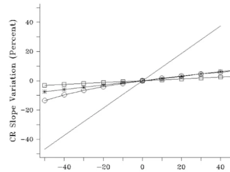
Figure 4 illustrates the percentage variation of the CR slope relative to its baseline value (∼3.8) as functions of per-centage variations in each of the four sensitivity parameters. Each of the latter is varied uniformly over a range of±50 % of the baseline values indicated in Table 1. It is immediately clear that the slope of the CR varies in a 1:1 manner with

γ. On the other hand, for the remaining three parameters, the percentage change in the CR slope is typically an order of magnitude smaller. We point out the nonlinearity associated with changing the surface drag coefficient, as decreasing sur-face drag produces a proportionately larger reduction in the slope of the CR compared to increasing surface drag by the same amount.

Since γ is just the slope of the Clausius–Clapeyron re-lationship, it has a quasi-exponential dependence on tem-perature and thus may be expected to vary sharply across the range of observed terrestrial temperature conditions. One consequence of this dependence is that the CR may be ex-pected to become more asymmetric with warming, as higher values of the slope imply a larger change in Ep for a given change in E. In turn, this may have implications for the strength of the coupling between the land surface and at-mosphere in a warming climate. For example, recent work by Dirmeyer et al. (2012, 2013, 2014) points to increases in metrics of land–atmosphere coupling strength in a warming climate. In Sect. 5, we further explore the response of our prototype to a global warming scenario.

In contrast to the complementary relationship, the Budyko curve exhibits no apparent change in shape for these param-eter variations. This shape invariance is unsurprising given that the Budyko curve is only a function of the aridity in-dexφ, as can be seen directly in the analytic solution for the analytic solution forη=2 (Eq. 15) or by substituting the ex-pression for runoff in Eq. (14). Thus, while E,Ep, andP vary in response to changing prototype parameters, their ra-tios are constrained to lie along a fixed Budyko curve. Yang et al. (2009) suggest such shape invariance is characteristic of the Budyko curve response to what they broadly term “cli-mate conditions”, as they note cli“cli-mate forcing at a particular location simply moves the system from one point along its characteristic Budyko curve to another. By contrast, Yang et al. (2009) show how different locations fall onto distinct Budyko curves as a result of land surface or landscape prop-erties such as soil, vegetation cover, rooting depth, etc. 4.2 Process intervention experiments

Apart from considering the sensitivity of the CR relationship (or Budyko curves) to parameter values, we can also assess how the prototype solutions respond to alteration of a par-ticular process or term in the governing equations. For the

Figure 4. Parameter sensitivity of the complementary relationship

slope. Results shown are for varying the slope of the saturation-specific humidity with respect to temperature (no symbols), surface drag coefficient (circles), surface cloud radiative forcing (stars), and convective adjustment timescale (squares).

first such intervention-type experiment, we alter the evap-otranspiration (E-intervention experiments) by prescribing as constant either (i) β or (ii) Ep. E-intervention experi-ment (i) is analogous to the methodology adopted in the Global Land Atmosphere Coupling Experiment (GLACE) type studies for comparing simulations with and without in-teractive soil moisture (Koster et al., 2004, 2006; Seneviratne et al., 2006).E-intervention experiment (ii) is similar to the approach Lintner et al. (2013) used to sever the feedback of near-surface climate ontoEp, which here is mediated prin-cipally through suppression of the dependence of potential evapotranspiration on “atmospheric drying power”, since the variation of radiative forcing across the prototype transect in its baseline configuration is weak (see discussion below).

Rather than present the complementary relationship for the

E-intervention experiments (since the CR necessarily breaks down in either case), we instead showTsandq as functions ofw(Fig. 5a and b, respectively). ForE-intervention exper-iment (i) withβ prescribed, the variation in Ts across soil moisture conditions (gray curve) is considerably reduced: while the difference in the baselineTs(black curve) between the driest and wettest conditions is roughly 5 K, it is under 0.5 K withβ prescribed. Similarly, the range of variation in specific humidity (here scaled to its surface value) across soil moisture states is attenuated relative to the baseline, although it is less pronounced than for surface temperature. Qualita-tively opposite behavior is seen underE-intervention experi-ment (ii) withEpprescribed, as the variations of bothTsand q across the rangeware increased relative to their baseline values. Note that at low soil moisture, the behavior of the baseline case more closely resemblesEpprescribed experi-ments, while at high soil moisture, it is more similar to theβ

Figure 5. Comparison of prototype (a) surface temperatureTsand (b) surface air humidityqafor the baseline (black), fixedβ(gray), and

fixedEp(blue) configurations of the prototype. Note thatqais converted to temperature units of K.

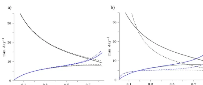
Figure 6. Impact on the complementary relationship from prescribing either (a) net surface radiative heating or (b) sensible heat flux. The

curves depicted correspond toEp(black),E(gray), andP (blue) for the baseline configuration (solid) and prescribed radiative or sensible

heat fluxes (dashed).

We can further assess how the CR changes with interven-tion in either surface sensible heat H or surface radiative heating Rs, by prescribing either of these fluxes to a con-stant value. UnderRsintervention (Fig. 6a), there is little net change in the CR relative to the baseline over most of the range of soil moisture; however, at highw, both Ep andE are slightly increased. The increase in Ep arises through a slight elevation of surface radiation heating above the base-line state, since the negative effect of cloud shortwave forc-ing, i.e., more convective clouds leading to less surface short-wave heating, is absent. This in turn feeds back onto pre-cipitation, which is slightly enhanced. We further mention a competing effect, namely increased surface longwave forc-ing (and hence warmforc-ing) with increased water vapor and convective cloudiness. For the parameter values chosen, this effect loses out to the shortwave forcing. On the other hand, uncertainty in these parameter values, particularly the cloud forcing, could alter the balance of these two effects.

UnderH intervention (Fig. 6b), the CR is dramatically al-tered, asEpdrops off more rapidly with increasing soil mois-ture, whileErises faster at low soil moisture and then

flat-tens off. The quantitative details of the change in shape of

EpandEdepend on the value of the sensible heat flux pre-scribed. PlottingEpvs.E(not shown) yields a best fit linear regressive slope of∼28, consistent with the very asymmetric nature of the CR when the variation inHacross the transect is suppressed.

5 Impacts of global warming and large-scale irrigation 5.1 Global warming

cycle is complicated by changes in land use such as defor-estation and agricultural conversion and coupling to vegeta-tion (Lee et al., 2011).

Over the latter half of the twentieth century, several stud-ies have reported widespread decreases in pan evapora-tion (Lawrimore and Peterson, 2000; Hobbins et al., 2004; Roderick and Farquhar, 2004; Shen et al., 2009), which can be related toEp. Several hypotheses have been proposed to explain the decreasing trend in pan evaporation, including increasing precipitation reducing the vapor pressure deficit of the lower atmosphere, global dimming reducing short-wave radiative heating at the surface, and stilling of surface winds reducing the exchange coefficient. Van Heerwaarden et al. (2010) conducted an extensive set of sensitivity tests for each of these effects on the CR using a conceptual model of the diurnal terrestrial boundary layer. They concluded that “except over wet soils, the actual evapotranspiration is more sensitive to changes in soil moisture than to changes in short wave radiation so that global evaporation should have in-creased. Nevertheless, Wild et al. (2004) speculate that in the latter half of the 20th century, increased moisture transport from the oceans enhanced precipitation over land, but sup-pressed the evaporation – opposite to [their] expectations”.

Figure 7 depicts the effect on prototype hydroclimate of imposing a 2 K warming of the prescribed column-mean temperature. In this figure, differences between the 2 K warming configuration and the baseline are plotted against baseline values of w; also shown is the difference in soil moisture between the 2 K warming and baseline scenarios. Across the range of baseline soil moisture conditions, the imposed warming decreases Ep (black), since q itself in-creases. While E (gray) increases with warming at w, it decreases for w >0.5, which is consistent with the results of van Heerwaarden et al. (2010). In addition, P (blue) in-creases under warming over the entire range of precipitation values (similar to Wild et al., 2004), albeit with a local mini-mum at intermediate soil moisture values.

The opposing changes ofEpandEwith warming at low soil moisture are consistent with expectations from the CR, as an increase in one corresponds to a decrease in the other. Of course, increasing the temperature increases the value of

γ, which means the slope of the CR increases between the baseline and 2 K warming scenarios. On the other hand, since

Ewet decreases with tropospheric warming, bothEp andE follow the behavior ofEwetand therefore decrease.

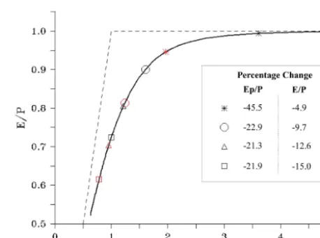
While the values of hydroclimatic variables may change substantially between the baseline and 2 K warming scenar-ios, the Budyko curve is unaltered, as discussed in Sect. 4.1. However, as Fig. 8 illustrates, forcing conditions, i.e., the value of drying advection, identified with specific points along the Budyko curve in the baseline scenario are shifted to lower values of the aridity indexφin the 2 K warming sce-nario, sinceEpdecreases whileP increases. Based on these results, we note the potential utility of the Budyko curve in

Figure 7. Differences inEp(black),E(gray), andP (blue) for a

+2 K warming relative to the baseline configuration as functions of soil moisture in the baseline configuration. Also shown is the difference in soil moisture (dashed black), which has been rescaled by a factor of 10.

Figure 8. Shift in selected points along the Budyko curve for the

baseline (black symbols) and+2 K warming (red) configuration. Pairs of like-shaped symbols correspond to the same level of im-posed drying advection forcing. The values shown in the inset are the percentage changes for each of the baseline and+2 K warming pairs.

providing qualitative or even quantitative constraints on how terrestrial hydroclimate variables will respond to warming. 5.2 Large-scale irrigation

Figure 9. Large-scale irrigation impacts on prototype hydroclimate. (a)Ep(black),E(gray), andP (blue) for the baseline (solid curves)

andI=2 mm day−1large-scale irrigation scenario (dotted curves), plotted with respect to horizontal moisture advection, scaled to units of mm day−1. Here, horizontal advection values correspond to drying advection, which are associated with decreasing precipitation. (b) As in

(a) but with soil moisture as the abscissa.

al. (2006) employed a mesoscale climate model and field data to demonstrate that large-scale irrigation in southeastern Turkey has impacted evaporation and potential evaporation in a complementary manner. They found a variety of inter-actions responsible for the trends, including increased atmo-spheric stability, decreased vapor pressure deficit, and, inter-estingly, a strong decrease in wind speed. Han et al. (2014) point out that while trends in Ep have often been invoked to estimate possible trends inE, how irrigation may impact

Ephas typically been neglected in the assessment and inter-pretation ofEptrends. It is thus worth briefly investigating how large-scale irrigation modulates the Budyko and com-plementary relationships within the framework of the proto-type analyzed here. To do this, we consider the addition of an irrigation source,I, to the soil moisture balance Eq. (6), which then becomesP+I=E+Qrunoff.

To see the impact of irrigation on the prototype hydro-climate, Fig. 9 depicts E, Ep, and P in the baseline and I =2 mm day−1configurations. Here, we have plotted these quantities with respect to both horizontal dry advection (Fig. 9a) and soil moisture (Fig. 9b). Given the direct moist-ening of the atmosphere by irrigation, the transition between nonprecipitating and precipitating conditions in the presence of irrigation occurs at a significantly larger value of drying advection in the large-scale irrigation scenario, as shown in Fig. 9a. Across the range of moisture advection values, both

E andP are enhanced in the presence of large-scale irriga-tion, as expected, andEpdecreases, in line with complemen-tarity. Additionally, at low to intermediate precipitation, E

exceedsP. Thus, whatever soil moisture is not locally recy-cled as precipitation would instead be transported downwind, as suggested by some studies on observed irrigation (e.g., DeAngelis et al., 2010). Viewed with respect to soil moisture (Fig. 9b), the inclusion of large-scale irrigation is seen to in-duce a slight increase inE for a given value of w. On the

other hand, since the value of drying advection is larger at a givenwin the presence of irrigation,Epitself is larger. Di-rectly relatingEptoEindicates effectively no change in the slope of the CR, though the intercept is increased when irri-gation is applied (not shown). Precipitation at a given value ofwis lowered in the irrigated scenario.

As a consequence of the changes inEandP, the Budyko curve for irrigated conditions (Fig. 10, dotted line) is shifted above its baseline: in fact, the irrigated Budyko curve extends above 1 forφ >1, as water limitation is effectively alleviated with the imposed irrigation water source. WhenEis replaced by the residualE∗=E−I, the resulting Budyko-like curve (stars) drops below the baseline.

Of course, we should point out that by imposing irrigation in the prototype with tropospheric temperature prescribed, we are neglecting a potentially important cooling of the low-ermost atmosphere, not to mention that our prototype does not account for changes in convective initiation or triggering that may occur, e.g., through changes to atmospheric stability (Findell et al., 2011). Moreover, we do not take into account vegetation control onEsince we only represent soil moisture dependence of evapotranspiration through a bucket model. Thus, the irrigation impacts described here merely reflect the direct effect of added moisture to the atmosphere.

6 Summary and conclusions

straightfor-Figure 10. Comparison of Budyko curves for the baseline (solid)

and I=2 mm day−1 (dotted) configurations. Also shown is a

Budyko-like curve in whichEis replaced byE∗=E−I(stars).

ward diagnosis of the sensitivity of the Budyko and com-plementary relationships to atmospheric and land surface pa-rameters. In particular, the slope of the CR is shown to be mostly dependent on the temperature, with important impli-cations for the continental hydrologic cycle with a warming climate. One consequence of this dependence is that the CR may be expected to become more asymmetric with warming, as higher values of the slope imply a larger change in po-tential evaporation for a given change in evapotranspiration. On the other hand, the Budyko curve is very stable to many parameterizations of the model parameters or global temper-ature. It is thus expected that the Budyko curve should re-main relatively stable under a warming climate. Other causes of anthropogenic changes such as large-scale irrigation are however shown to strongly impact the Budyko curve, with little impact on the CR.

Acknowledgements. This work was supported by National Science Foundation (NSF) grant AGS-1035968 and New Jersey Agricul-tural Experiment Station Hatch grant NJ07102.

Edited by: V. Andréassian

References

Allen, M. R. and Ingram, W. J.: Constraints on future changes in climate and the hydrologic cycle, Nature, 419, 224–232, doi:10.1038/nature01092, 2002.

Betts, A. K.: Coupling of water vapor convergence, clouds, pre-cipitation, and land-surface processes, J. Geophys. Res., 112, D10108, doi:10.1029/2006JD008191, 2007.

Betts, A. K. and Miller, M. J.: A new convective adjustment scheme. Part II: Single column tests using GATE wave, BOMEX, ATEX

and arctic air-mass data sets, Q. J. Roy. Meteor. Soc., 112, 693– 709, doi:10.1002/qj.49711247308, 1986.

Betts, A. K. and Viterbo, P.: Land-surface, boundary layer, and cloud-field coupling over the southwestern Amazon in ERA-40, J. Geophys. Res., 110, D14108, doi:10.1029/2004JD005702, 2005.

Betts, A. K., Ball, J., Beljaars, A., Miller, M. J., and Viterbo, P.: The land surface–atmosphere interaction: a review based on observa-tional and global modeling perspectives, J. Geophys. Res., 101, 7209–7225, doi:10.1029/95JD02135, 1996.

Betts, A. K., Ball, J. H., Bosilovich, M., Viterbo, P., and Zhang, Y.: Intercomparison of water and energy budgets for five Mis-sissippi subbasins between ECMWF reanalysis (ERA-40) and NASA Data Assimilation Office GCM for 1990, J. Geophys. Res., 108, 8618, doi:10.1029/2002JD003127, 2003.

Betts, A. K., Desjardins, R., Worth, D., Wang, S., and Li, J.: Coupling of winter climate transitions to snow and clouds over the Prairies, J. Geophys. Res.-Atmos., 119, 1118–1139, doi:10.1002/2013JD021168, 2014.

Bosman, H. H.: The influence of installation practices on evapora-tion from Symon’s tank and American Class A-pan evaporime-ters, Agr. Forest Meteorol., 41, 307–323, 1987.

Bouchet, R.: Evapotranspiration reelle et potentielle, signification climatique, IAHS Publ., 62, 134–142, 1963 (in French). Brutsaert, W. and Parlange, M. B.: Hydrologic cycle explains the

evaporation paradox, Nature, 396, 29–30, 1998.

Brutsaert, W. and Stricker, H.: An advection-aridity approach to estimate actual regional evapotranspiration, Water Resour. Res., 15, 443–450, 1979.

Budyko, M. I.: The heat and water balance of the Earth’s sur-face, the general theory of physical geography and the prob-lem of the transformation of nature, Sov. Geogr., 2, 3–12, doi:10.1080/00385417.1961.10770737, 1961.

Budyko, M. I.: Climate and Life, Academic Press, Orlando, FL, 508 pp., 1974.

Cook, B. I., Puma, M. J., and Krakauer, N. Y.: Irrigation duced surface cooling in the context of modern and in-creased greenhouse gas forcing, Clim. Dynam., 37, 1587–1600, doi:10.1007/s00382-010-0932-x, 2010.

Crago, R. and Crowley, R.: Complementary relationships for near-instantaneous evaporation, J. Hydrol., 300, 199–211, doi:10.1016/j.jhydrol.2004.06.002, 2005.

DeAngelis, A., Dominguez, F., Fan, Y., Robock, A., Kustu, M. D., and Robinson, D.: Evidence of enhanced precipitation due to ir-rigation over the Great Plains of the United States, J. Geophys. Res., 115, D15115, doi:10.1029/2010JD013892, 2010.

Dirmeyer, P. A., Cash, B. A., Kinter III, J. L., Stan, C., Jung, T., Marx, L., Towers, P., Wedi, N., Adams, J. M., Altshuler, E. L., Huang, B., Jin, E. K., and Manganello, J.: Evidence for enhanced land–atmosphere feedback in a warming climate, J. Hydromete-orol., 13, 981–995, doi:10.1175/JHM-D-11-0104.1, 2012. Dirmeyer, P. A., Jin, Y., Singh, B., and Yan, X.: Trends in land–

atmosphere interactions from CMIP5 simulations, J. Hydrome-teor., 14, 829–849, doi:10.1175/JHM-D-12-0107.1, 2013. Dirmeyer, P. A., Wang, Z., Mbuh, M. J., and Norton, H. E.:

Donohue, R. J., Roderick, M. L., and McVicar, T. R.: On the importance of including veg30 etation dynamics in Budyko’s hydrological model, Hydrol. Earth Syst. Sci., 11, 983–995, doi:10.5194/hess-11-983-2007, 2007.

Eagleson, P.: Climate, soil, and vegetation, 2. The distribution of an-nual precipitation derived from observed storm sequences, Water Resour Res., 14, 713–721, 1978a.

Eagleson, P.: Climate, soil, and vegetation, 6. Dynamics of the an-nual water balance, Water Resour. Res., 14, 749–764, 1978b. Eagleson, P.: Climate, soil, and vegetation, 1. Introduction to water

balance dynamics, Water Resour. Res., 14, 705–712, 1978c. Findell, K. L., Gentine, P., Lintner, B. R., and Kerr, C.:

Prob-ability of afternoon precipitation in eastern US and Mexico enhanced by high evaporationm, Nat. Geosci., 4, 434–439, doi:10.1038/ngeo1174, 2011.

Fu, B. P.: On the calculation of the evaporation from land surface, Sci. Atmos. Sin, 5, 23–31, 1981.

Gentine, P., Entekhabi, D. D., and Polcher, J.: The diurnal be-havior of evaporative fraction in the soil-vegetation-atmospheric boundary layer continuum, J. Hydrometeorol., 12, 1530–1546, doi:10.1175/2011JHM1261.1, 2011.

Gentine, P., D’Odorico, P., Lintner, B. R., Sivandran, G., and Salvucci, G.: Interdependence of climate, soil, and vegetation as constrained by the Budyko curve. Geophys. Res. Lett., 39, L19404, doi:10.1029/2012GL053492, 2012.

Gerrits, A. M. J., Savenije, H. H. G., Veling, E. J. M., and Pfister, L.: Analytical derivation of the Budyko curve based on rainfall characteristics and a simple evaporation model, Water Resour. Res., 45, W04403, doi:10.1029/2008WR007308, 2009. Granger, R. J.: A complementary relationship approach for

evapo-ration from nonsaturated surfaces, J. Hydrol., 111, 31–38, 1989. Guimberteau, M., Laval, K., Perrier, A., and Polcher, J.: Global ef-fect of irrigation and its impact on the onset of the Indian summer monsoon, Clim. Dynam., 39, 1329–1348, doi:10.1007/s00382-011-1252-5, 2011.

Han, S., Tang, Q., Xu, D., and Wang, S.: Irrigation-induced changes in potential evaporation: more attention is needed, Hydrol. Pro-cess., 28, 2717–2720, doi:10.1002/hyp.10108, 2014.

Harman, C. J., Troch, P. A., and Sivapalan, M.: Functional model of water balance variability at the catchment scale: 2. Elasticity of fast and slow runoff components to precipitation change in the continental United States, Water Resour. Res., 47, W02523, doi:10.1029/2010WR009656, 2011.

Held, I. M. and Soden, B. J.: Robust response of the hydrological cycle to global warming, J. Climate, 19, 5686–5699, 2006. Hobbins, M. T., Ramirez, J. A., Brown, T. C., and Claessens,

L. H. J. M.: The complementary relationship in estimation of re-gional evapotranspiration: the complementary relationship area evapotranspiration and advection-aridity models, Water Resour. Res., 37, 1367–1387, 2001.

Hobbins, M. T., Ramirez, J. A., and Brown, T. C.: Trends in pan evaporation and actual evapotranspiration across the contermi-nous US: paradoxical or complementary?, Geophys. Res. Lett., 31, L13503, doi:10.1029/2004GL019846, 2004.

Istanbulluoglu, E., Wang, T., Wright, O. M., and Lenters, J. D.: In-terpretation of hydrologic trends from a water balance perspec-tive: the role of groundwater storage in the Budyko hypothesis, Water Resour. Res., 48, W00H16, doi:10.1029/2010WR010100, 2012.

Kahler, D. M. and Brutsaert, W.: Complementary relationship be-tween daily evaporation in the environment and pan evaporation, Water Resour. Res., 42, W05413, doi:10.1029/2005WR004541, 2006.

Koster, R. and Suarez, M.: A simple framework for examining the interannual variability of land surface moisture fluxes, J. Climate, 12, 1911–1917, 1999.

Koster, R. D., Dirmeyer, P. A., Guo, Z., Bonan, G., Chan, E., Cox, P., Davies, H., Gordon, T., Kanae, S., Kowalczyk, E., Lawrence, D., Liu, P., Lu, S., Malyshev, S., McAvaney, B., Mitchell, K., Oki, T., Oleson, K., Pitman, A., Sud, Y., Taylor, C., Verseghy, D., Vasic, R., Xue, Y., and Yamada, T.: Regions of strong coupling between soil moisture and precipitation, Science, 305, 1138– 1140, 2004.

Koster, R. D., Guo, Z., Dirmeyer, P. A., Bonan, G., Chan, E., Cox, P., Davies, H., Gordon, T., Kanae, S., Kowalczyk, E., Lawrence, D., Liu, P., Lu, S., Malyshev, S., McAvaney, B., Mitchell, K., Oki, T., Oleson, K., Pitman, A., Sud, Y., Taylor, C., Verseghy, D., Vasic, R., Xue, Y., and Yamada, T.: GLACE: the Global Land– Atmosphere Coupling Experiment, Part I: Overview, J. Hydrom-eteorol., 7, 590–610, 2006.

Kirchner, J. W.: Catchments as simple dynamical systems: catchment characterization, rainfall–runoff modeling, and do-ing hydrology backward, Water Resour. Res., 45, W02429, doi:10.1029/2008WR006912, 2009.

Lawrimore, J. and Peterson, T.: Pan evaporation trends in dry and humid regions of the United States, J. Hydrometeorol., 1, 543– 546, 2000.

Lee, J.-E., Lintner, B. R., Boyce, C. K., and Lawrence, P. J.: Land use change exacerbates tropical South American drought by sea surface temperature variability, Geophys. Res. Lett., 38, L19706, doi:10.1029/2011GL049066, 2011.

Lettau, H.: Evapotranspiration climatonomy, I. A new approach to numerical prediction of monthly evapotranspiration, runoff, and soil moisture storage, Mon. Weather Rev., 97, 691–699, 1969. L’homme, J. and Guilioni, L.: Comments on some articles

about the complementary relationship, J. Hydrol., 323, 1–3, doi:10.1016/j.jhydrol.2005.08.014, 2006.

Lintner, B. R., Gentine, P., Findell, K. L., D’Andrea, F., Sobel, A. H., and Salvucci, G. D.: An idealized prototype for large-scale land–atmosphere coupling, J. Climate, 26, 2379–2389, doi:10.1175/JCLI-D-11-00561.1, 2013.

Milly, P. C. D.: Climate, soil water storage, and the average annual water balance, Water Resour. Res., 30, 2143–2156, 1994. Milly, P. C. D. and Dunne, K.: Macroscale water fluxes – 2. Water

and energy supply control of their interannual variability, Water Resour. Res., 38, 1206, doi:10.1029/2001WR000760, 2002. Milly, P. C. D., Dunne, K., and Vecchia, A. V.: Global pattern of

trends in streamflow and water availability in a changing climate, Nature, 438, 347–350, doi:10.1038/nature04312, 2005. Morton, F. I.: Operational estimates of areal evapotranspiration and

their significance to the science and practice of hydrology, J. Hy-drol., 66, 1–76, 1983.

Neelin, J. D. and Zeng, N.: A quasi-equilibrium tropical circulation model–formulation, J. Atmos. Sci., 57, 1741–1766, 2000. Neelin, J. D., Munnich, M., Su, H., Meyerson, J., and Holloway, C.:

Ozdogan, M., Salvucci, G., and Anderson, B.: Examination of the Bouchet–Morton complementary relationship using a mesoscale climate model and observations under a progressive irrigation scenario, J. Hydrometeorol., 7, 235–251, 2006.

Pettijohn, J. C. and Salvucci, G. D.: A new two-dimensional physical basis for the complementary relation between ter-restrial and pan evaporation, J. Hydrometeorol., 10, 565–574, doi:10.1175/2008JHM1026.1, 2009.

Porporato, A., Laio, F., Ridolfi, L., and Rodríguez-Iturbe, I.: Plants in water-controlled ecosystems: active role in hydrologic pro-cesses and response to water stress – III. Vegetation water stress, Adv. Water Resour., 24, 725–744, 2001.

Porporato, A., Daly, E., and Rodríguez-Iturbe, I.: Soil water balance and ecosystem response to climate change, Am. Nat., 164, 625– 632, 2004.

Potter, N., Zhang, L., Milly, P., McMahon, T., and Jakeman, A.: Effects of rainfall seasonality and soil moisture capacity on mean annual water balance for Australian catchments, Water Resour. Res., 41, W06007, doi:10.1029/2004WR003697, 2005. Priestley, C. H. B. and Taylor, R. J.: On the assessment of surface

heat flux and evaporation using large-scale parameters, Mon. Weather Rev., 100, 81–88, 1972.

Ramirez, J. A., Hobbins, M. T., and Brown, T. C.: Observational evidence of the complementary relationship in regional evapo-ration lends strong support for Bouchet’s hypothesis, Geophys. Res. Lett., 32, L15401, doi:10.1029/2005GL023549, 2005. Roderick, M. L. and Farquhar, G. D.: Changes in Australian pan

evaporation from 1970 to 2002, Int. J. Climatol., 24, 1077–1090, doi:10.1002/joc.1061, 2004.

Roderick, M. L. and Farquhar, G. D.: A simple framework for re-lating variations in runoff to variations in climatic conditions and catchment properties, Water Resour. Res., 47, W00G07, doi:10.1029/2010WR009826, 2011.

Seneviratne, S. I., Koster, R. D., Guo, Z., Dirmeyer, P. A., Kowal-czyk, E., Lawrence, D., Liu, P., Lu, C.-H., Mocko, D., Oleson, K. W., and Verseghy, D.: Soil moisture memory in AGCM sim-ulations: analysis of Global Land–Atmosphere Coupling Exper-iment (GLACE) data, J. Hydrometeorol., 7, 1090–1112, 2006. Shen, Y., Liu, C., Liu, M., Zeng, Y., and Tian, C.: Change in pan

evaporation over the past 50 years in the arid region of China, Hydrol. Process., 24, 225–231, doi:10.1002/hyp.7435, 2009. Sherwood, S. and Fu, Q.: A drier future?, Science, 343, 737–739,

doi:10.1126/science.1247620, 2014.

Sivapalan, M., Yaeger, M. A., Harman, C. J., Xu, X., and Troch, P. A.: Functional model of water balance variability at the catchment scale: 1. Evidence of hydrologic similarity and space- time symmetry, Water Resour. Res., 47, W02522, doi:10.1029/2010WR009568, 2011.

Sobel, A. H. and Bretherton, C. S.: Modeling tropical precipitation in a single column, J. Climate, 13, 4378–4392, 2000.

Sobel, A. H., Nilsson, J., and Polvani, L.: The weak temperature gradient approximation and balanced tropical moisture waves, J. Atmos. Sci., 58, 3650–3665, 2001.

Szilagyi, J.: On Bouchet’s complementary hypothesis, J. Hydrol., 246, 155–158, 2001.

Szilagyi, J.: On the inherent asymmetric nature of the comple-mentary relationship of evaporation, Geophys. Res. Lett., 34, L02405, doi:10.1029/2006GL028708, 2007.

Szilagyi, J. and Jozsa, J.: Complementary relationship of evapora-tion and the mean annual water-energy balance, Water Resour. Res., 45, W09201, doi:10.1029/2009WR008129, 2009. Troch, P. A., Martinez, G. F., Pauwels, V. R. N., Durcik, M.,

Siva-palan, M., Harman, C., Brooks, P. D., Gupta, H., and Huxman, T.: Climate and vegetation water use efficiency at catchment scales, Hydrol. Process., 23, 24090–2414, doi:10.1002/hyp.7358, 2009. Tuttle, S. E. and Salvucci, G. D.: A new method for cali-brating a simple, watershed-scale model of evapotranspira-tion: maximizing the correlation between observed streamflow and modelinferred storage, Water Resour. Res., 48, W05556, doi:10.1029/2011WR011189, 2012.

van Heerwaarden, C. C., Vilà-Guerau de Arellano, J., and Teul-ing, A. J.: Land–atmosphere coupling explains the link be-tween pan evaporation and actual evapotranspiration trends in a changing climate, Geophys. Res. Lett., 37, L21401, doi:10.1029/2010GL045374, 2010.

Wild, M., Ohmura, A., Gilgen, H., and Rosenfeld, D.: On the con-sistency of trends in radiation and temperature records and im-plications for the global hydrological cycle, Geophys. Res. Lett., 31, L11201, doi:10.1029/2003GL019188, 2004.

Williams, C. A., Reichstein, M., Buchmann, N., Baldocchi, D., Beer, C., Schwalm, C., Wohlfahrt, G., Hasler, N., Bernhofer, C., Foken, T., Papale, D., Schymanski, S., and Schaefer, K.: Climate and vegetation controls on the surface water bal-ance: synthesis of evapotranspiration measured across a global network of flux towers, Water Resour. Res., 48, W06523, doi:10.1029/2011WR011586, 2012.

Yang, D., Sun, F., Liu, Z., Cong, Z., Ni, G., and Lei, Z.: Analyz-ing spatial and temporal variability of annual water-energy bal-ance in nonhumid regions of China using the Budyko hypothesis, Water Resour. Res., 43, W04426, doi:10.1029/2006WR005224, 2007.

Yang, D., Shao, W., Yeh, P. J.-F., Yang, H., Kanae, S., and Oki, T.: Impact of vegetation cover age on regional water balance in the nonhumid regions of China, Water Resour. Res., 45, W00A14, doi:10.1029/2008WR006948, 2009.

Yang, H., Yang, D., Lei, Z., and Sun, F.: New analytical derivation of the mean annual waterenergy balance equation, Water Resour. Res., 44, W03410, doi:10.1029/2007WR006135, 2008. Zanardo, S., Harman, C. J., Troch, P. A., Rao, P. S. C., and

Siva-palan, M.: Intra-annual rainfall variability control on interan-nual variability of catchment water balance: a stochastic analysis, Water Resour. Res., 48, W00J16, doi:10.1029/2010WR009869, 2012.

Zeng, N., Neelin, J. D., and Chou, C.: A quasi-equilibrium tropi-cal circulation model–implementation and simulation, J. Atmos. Sci., 57, 1767–1796, 2000.