www.hydrol-earth-syst-sci.net/20/3263/2016/ doi:10.5194/hess-20-3263-2016
© Author(s) 2016. CC Attribution 3.0 License.
Cloud tolerance of remote-sensing technologies to
measure land surface temperature
Thomas R. H. Holmes1,2, Christopher R. Hain3, Martha C. Anderson1, and Wade T. Crow1
1Hydrology and Remote Sensing Lab., USDA-ARS, Beltsville, MD, USA
2Hydrological Sciences Laboratory, NASA Goddard Space Flight Center, Greenbelt, MD, USA 3Earth Science Interdisciplinary Center, University of Maryland, College Park, MD, USA
Correspondence to:Thomas R. H. Holmes ([email protected])
Received: 13 April 2016 – Published in Hydrol. Earth Syst. Sci. Discuss.: 21 April 2016 Revised: 1 July 2016 – Accepted: 21 July 2016 – Published: 11 August 2016
Abstract. Conventional methods to estimate land surface temperature (LST) from space rely on the thermal infrared (TIR) spectral window and is limited to cloud-free scenes. To also provide LST estimates during periods with clouds, a new method was developed to estimate LST based on passive-microwave (MW) observations. The MW-LST product is informed by six polar-orbiting satellites to create a global record with up to eight observations per day for each 0.25◦ resolution grid box. For days with sufficient observations, a continuous diurnal temperature cycle (DTC) was fitted. The main characteristics of the DTC were scaled to match those of a geostationary TIR-LST product.
This paper tests the cloud tolerance of the MW-LST prod-uct. In particular, we demonstrate its stable performance with respect to flux tower observation sites (four in Europe and nine in the United States), over a range of cloudiness condi-tions up to heavily overcast skies. The results show that TIR-based LST has slightly better performance than MW-LST for clear-sky observations but suffers an increasing negative bias as cloud cover increases. This negative bias is caused by incomplete masking of cloud-covered areas within the TIR scene that affects many applications of TIR-LST. In contrast, for MW-LST we find no direct impact of clouds on its ac-curacy and bias. MW-LST can therefore be used to improve TIR cloud screening. Moreover, the ability to provide LST estimates for cloud-covered surfaces can help expand cur-rent clear-sky-only satellite retrieval products to all-weather applications.
1 Introduction
Information about the land surface temperature (LST) is an important element in the retrieval of many hydrological states and fluxes from satellite-measured radiances. For example, the retrieval of soil moisture or precipitation from passive-microwave observations requires a coincident estimate of LST (e.g., Owe et al., 2008). In other applications, the rate of change in temperature is contrasted with net radiation to estimate evaporation as a residual of the surface energy bal-ance (e.g., Anderson et al., 2011).
The most direct way to estimate LST from spaceborne in-struments is by radiometers which measure within the ther-mal infrared (TIR) band of the electromagnetic spectrum. Thermal emission within this frequency band can be related directly to the physical temperature of the land surface and is more precisely termed the ensemble radiometric tempera-ture (Norman and Becker, 1995). Spaceborne TIR radiome-ters allow for very high spatial resolution imagery. Even at the height of geostationary platforms radiometers can deliver 3 km spatial resolution, e.g., the Spinning Enhanced Visible and Infrared Imager (SEVIRI). A drawback to the TIR tech-nique is that – at such wavelengths – clouds completely block the emission from the land surface. This means that space-borne TIR radiometers give no information about the land surface below the clouds and instead reflect the temperature and emissivity of the clouds. The result is that the quality of the cloud screening directly affects the quality of a TIR-LST product.
partic-ular the Ka-band (∼37 GHz) was shown to have a strong link with LST (Owe and Van de Griend, 2001). Based on these observations, linear-regression-based LST estimates were derived for the Ka-band (Holmes et al., 2009), and variants of these linear relations are currently used in soil moisture retrieval (Jackson et al., 1999; Owe et al., 2008). However, using a single linear regression across the globe ig-nores potentially significant differences in microwave emis-sivity and can result in large biases, especially in desert ar-eas. It also cannot account for large differences in the am-plitude of the diurnal cycle between MW- and TIR-based LST, which have been implicated in reduced soil moisture retrieval skill during daylight hours (Lei et al., 2015; Pari-nussa et al., 2011). In contrast to these relatively simple linear methods, a neural network method was developed by Aires et al. (2001) to estimate LST based on multiple microwave channels besides Ka-band. By using atmospheric and sur-face information in addition to TIR-LST in the training of the scheme, this method minimized systematic bias in monthly mean temperatures. However, because the training is based on a single polar-orbiting satellite, it cannot give diurnal tem-perature information. Both of these methods were compared with station data by Catherinot et al. (2011), giving strong confirmation on the lack of sensitivity of microwave-based LST estimates to cloud liquid water path. This method has recently been developed further to allow for more continu-ous application to a more diverse suite of satellites and over-pass times (Prigent et al., 2016). One drawback to all over- passive-microwave-based methods is relatively coarse spatial resolu-tion as compared to TIR sensors. At Ka-band, the smallest footprint size currently achieved with polar-orbiting satellites is 10×15 km.
Because of the complementary nature of TIR- and MW-based LST, there is a clear interest in merging these two in-dependent technologies. For example, TIR-LST-based evap-oration retrievals would benefit from observational data dur-ing cloudy periods (e.g., Anderson et al., 2011). On the other hand, microwave soil moisture retrievals from Soil Moisture Active Passive (SMAP) have the goal of 9 km spatial resolu-tion, and this poses a resolution challenge to MW-LST inputs if TIR-LST cannot be leveraged. Reconciling the systematic differences in diurnal temperature cycle (DTC) between TIR and Ka-band is the first step towards an ultimate merger into a diurnally continuous LST product. To do this, Holmes et al. (2015) developed a method to scale the diurnal charac-teristics of a multi-satellite dataset of Ka-band observations to a TIR-LST product with 15 min temporal sampling from geostationary satellites. This scaling was able to account for biases in characteristics of the DTC related to Ka-band emis-sivity, sensing depth and atmospheric effects (Holmes et al., 2015). By explicitly taking account of systematic differences in DTC between TIR and Ka-band, this method is able to estimate LST at any time of day from sparse Ka-band ob-servations. Note that a similar pixel-by-pixel approach was
applied by André et al. (2015) over the Arctic region where a single satellite can provide diurnal sampling.
The aim of this paper is to evaluate the new global MW-LST dataset in comparison with existing TIR-MW-LST data over clear-sky days and particularly to test the assumption that MW-LST is tolerant to high levels of cloud coverage. Ground observations provide a common benchmark to test the rela-tive accuracy of the two satellite products. Because the di-urnal MW-LST product (Holmes et al., 2015) was scaled to TIR-based LST as produced by the Land Surface Analysis Satellite Application Facility (LSA-SAF; see http://landsaf. meteo.pt), the evaluation is mostly concerned with tempo-ral precision, not with absolute bias. In previous work it was shown that relative aspects of a coarse-scale product can be evaluated using sparse in situ observations (Holmes et al., 2012). For a thorough discussion of absolute accuracy, read-ers are referred to papread-ers detailing validation exercises for LSA-SAF-LST (e.g., Ermida et al., 2014; Göttsche et al., 2013, 2016).
After establishing the accuracy of MW-LST relative to TIR-LST for a particular site, the stability of the precision of MW-LST (relative to ground data) for increasing cloudiness will be tested. Previous work showed indications of cloud tolerance of MW-LST in comparison to TIR-LST (Holmes et al., 2015), but the analysis used proxies for both cloud cover and LST quality. In this paper we use a more direct estimate of cloudiness and provide a more detailed look at the valida-tion statistics for different levels of daytime cloudiness with the ground station as the reference. The hypothesis we test is that clouds affect a satellite-measured LST by introduc-ing an error (E). If E is consistent in sign throughout the measurement period (e.g., if clouds always lower the satel-lite LST estimate), this will introduce a systematic bias that will increase with cloud cover. If on the other hand the sign ofEvaries, it will increase the random error in LST, but not necessarily a systematic bias. Only if we do not see a sys-tematic bias with increasing cloud cover, nor an increase in random error, can we reject the hypothesis that clouds affect the satellite LST.
2 Materials
2.1 Satellite LST estimates: thermal infrared
Anal-ysis, Satellite Application Facility (LSA-SAF) produces op-erational LST products based on split-window observations (channels centered at 10.8 and 12.0 µm) of MSG-9. LSA-SAF-LST is originally produced at 3 km spatial resolution. For this study, the data are aggregated to match the 0.25◦ resolution of MW-LST. If two-thirds of the 3 km observa-tions are masked, then the sample average is rejected for that location and time.
For North America, NOAA operates the Geostationary Operational Environmental Satellites (GOES). GOES Sur-face and Insulation Products (GSIP) are produced by the Of-fice of Satellite Data Processing and Distribution (OSPO), National Environmental Satellite Data and Information Ser-vice (NESDIS), NOAA, and include LST (V3 was used for this study). Unlike MSG-based LST, GOES GSIP LST is based on a dual-window technique (3.9 and 11.0 µm) rather than the preferred split-window technique due to the lack of a 12µthermal channel on the current generation of the GOES imager. An operational hourly LST at 0.125◦spatial resolu-tion is available from 2 April 2009 onwards. For this study, we averaged the nine 0.125◦ nodes that cover the edge and center of the 0.25◦MW-LST product grid cell. In order to further reduce possible cloud contamination, a particular data point is only used if all nine 0.125◦pixels covering the 0.25◦ grid box contain (non-cloud-masked) data.
2.2 Satellite LST estimates: microwave
The MW-LST product is based on vertical polarized Ka-band (36–37 GHz) brightness temperature (TKa)as measured by microwave radiometers on six satellites in low Earth or-bit. These satellites include the Advanced Microwave Scan-ning Radiometer on EOS (AMSR-E) to October 2011 and its successor on AMSR2 from July 2012. Also included are the Special Sensor Microwave and Imager (SSM/I) on plat-forms F13, F14 and F15 of the Defense Meteorological Satel-lite Program; the Tropical Rainfall Measurement Mission (TRMM) Microwave Imager (TMI); and Coriolis-WindSat. These observations are combined to create a global record with up to eight observations per day for each 0.25◦ resolu-tion grid box. The data are binned in 15 min windows of local solar time (00:00–00:15 is the first window of the day). The brightness temperatures are intercalibrated using observa-tions from the TRMM satellite (with an equatorial overpass) as a transfer reference. Individual 0.25◦averages are masked if the spatial standard deviation of the oversampled Ka-band observations exceeds a prior determined threshold for a given grid box. Both the intercalibration and quality control proce-dures are described in detail in Holmes et al. (2013a).
The methodology to estimate LST from this record of Ka-band observations is described in Holmes et al. (2015) and summarized below. For days with suitable observations (a minimum of four, including at least one within a third day length from solar noon) and noTKa<250 K (an indication of frozen soil), a continuous DTC is fitted. The DTC model
used is based on Göttsche and Olesen (2001) with slight adaptations to limit the number of parameters. This imple-mentation (DTC3) is fully described in Holmes et al. (2015). DTC3 summarizes the DTC with two daily parameters (daily minimum T0 at the start and end of the day, and diurnal
amplitudeA)together with diurnal timing (ϕ), which is as-sumed a temporal constant (Holmes et al., 2013b). The daily mean is defined by the daily minimum and the amplitude (T =T0+A/2). The Ka-band DTC parameters for
individ-ual days (TKad ,AKad )are scaled to match the long-term mean of TIR observations:
AMWd =AKad /δ, (1)
TMWd =β0+β1T Ka
d . (2)
The scaled parameters are indicated with the superscript “MW”. The parameterδ represents the slope of the zero-order least-squares regression line for estimating the am-plitude of AKad from TIR-LST (ATIRd ). The intercept (β0)
and slope (β1)to correct the mean daily temperature (T Ka d )
for systematic differences with TIR-LST (TTIRd ) are deter-mined with a constrained numerical solver, as in Holmes et al. (2015). The constraint is based on radiative transfer con-siderations and assures that the scaling of the mean is in agreement with the prior scaling of the amplitude (Eq. 1). These scaling parameters were determined for each 0.25◦ grid box based on data for the period 2009–2012. The scal-ing (Eqs. 1 and 2) is applied to every day for which estimates ofTKa andAKa are available. Together with the timing of the diurnal cycle of TIR-LST,ϕTIR, as determined based on (Holmes et al., 2013b), we then calculate the diurnal MW-LST based on the same DTC3 model:
MW-LST=DTC3 ϕTIRT0MWAMW. (3) Comparing actual Ka-band observations to estimates pro-vided by the fitted DTC model provides a valuable means of quality control. The root mean square error (RMSE) of the misfit between the DTC3 model and the sparseTKa observa-tions is used to flag days where the assumpobserva-tions imposed by the shape of clear-sky DTC are not valid or individual Ka-band observations have a large bias.
Besides the continuous MW-LST product, we can also evaluate the product at the actual Ka-band observation times (thus weakening our reliance on the DTC3 model). To do this, we project the difference between the original MW data and the DTC model fit onto MW-LST. This product is re-ferred to as MW-LST-Sparse:
MW-LST-Sparse=DTC3 ϕTIR, T0MW, AMW +1
δ T
Ka−DTC3 ϕKa, TKa 0 , A
Ka
. (4)
differences between the observations and the diurnal model at the actual observation time are preserved. The difference between the continuous MW-LST and the MW-LST-Sparse is illustrated in Fig. 1 (lower panel).
2.3 Ground observations
FLUXNET is a worldwide network of meteorological mea-surement towers (flux tower) with common meamea-surement protocols (Baldocchi et al., 2001). Each flux tower includes an instrument positioned above the vegetation canopy to measure net radiation. This instrument is made up of two pyranometers to measure up- and downwelling shortwave radiation and two pyrgeometers to measure up- and down-welling longwave radiation. The radiometric surface tem-perature (T ) can be derived from the longwave radiation measurements (upwelling: L↑, W m−2; downwelling: L↓, W m−2)using the following equation:
L↑=εLσ T4+(1−εL) L↓, (5)
where εL is the broadband emissivity over the spectral
range of the pyrgeometer (4.5–42 µm) andσ is the Stefan– Boltzmann constant (σ =5.670×10⁻⁸W m−2K−1). 2.3.1 Longwave emissivity
An estimate of εL is obtained for each site based on
mea-surements of L↑ together with additional measurements of screen level air temperature (Ta), sensible heat flux (H )and
wind speed (u). This estimate is based on three assumptions: (1)His directly proportional to the near-surface temperature gradient, (2) the differenceT−Tarepresents that temperature
gradient and (3)H=0 when there is no vertical temperature gradient (i.e.,T =Ta). With these three assumptions in mind
we then iterate overεLto find the solution where the
regres-sion ofHagainst (T−Ta)goes through zero and the squared
errors are minimized. When measurements of wind speed are available, they are used to select atmospheric conditions where the relationship betweenHand the near-surface tem-perature gradient is strongest (u> 2 m s−1). For forest sites, the direct relationship between H and T gradients breaks down. In those cases, the simpler assumption is used that the long-term average of T andTa are equal: hTi = hTai. For
more discussion and examples of this method see Holmes et al. (2009). In this study we apply this method to determine monthlyεL for each site individually and then use the
me-dian value ofεL(listed in Table 1) to calculateT based on
Eq. (5). The standard deviation of the monthly measurements of εL is also listed in Table 1 and provides an indication of
both uncertainty and seasonal variation inεL.
2.3.2 Spatial representativeness and site selection The tower-based estimate of T, from (Eq. 5), directly rep-resents only the immediate tower surroundings within a
ra-dius of approximately 50 m. Clearly this is a very small spa-tial sampling of the 0.25◦ grid box (∼25×25 km)
repre-sented by the satellite LST estimates used in this study (see Sects. 2.1 and 2.2). As a consequence, we typically find large systemic differences between the station data and the areal average. Given that overall weather conditions are relatively homogenous over distances of 25 km, these differences can be attributed to the land cover type at the station location in comparison to that over the entire grid box (for examples of this, see Holmes et al., 2009). The representation of the spa-tial average by ground observations can be improved signif-icantly if more than one station is available in the same grid box and the towers are situated in thermodynamically con-trasting land cover types (forest and cropland/herbaceous). In that case the land cover associated with the tower site (sub-script, s) determines the weight (W ) according to the spa-tial fraction of that land cover type within the 0.25◦grid box
(MCD12C1; Friedl et al., 2010). We use this information to estimate the grid average LST as the weighted average of site-measuredT according to Eq. (6):
LST=
n
P
s=1
WsTs n
P
s=1
Ws
. (6)
For example, site DE-Hai of location A is located in a for-est and represents 16 % of the pixel. Site DE-Geb is located in croplands and represents 80 % of the pixel that has low vegetation cover or bare soil. Urban, open water or wetland accounts for the remaining 4 %, which does not affect the weighting. We only considered locations where this rest frac-tion is below 5 % of the grid coverage. Another criterion for site selection was that the land cover at the site must repre-sent more than 75 % of the pixel. Sites in mountainous areas are also excluded. For the period of 2009–2012 this means there are 13 locations with at least 2 years of flux tower sites available for this study, and four of these locations contain multiple stations. For pixels where only one station is avail-able, LST is set equal to the site measurement: LST=T. All the validation targets are listed in Table 1, together with the geographic location of the individual stations, the land cover type as reported by the flux tower operators and the parame-tersWandεLas described above.
2.3.3 Cloudiness at tower location
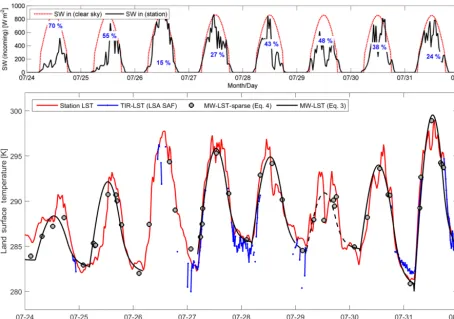
Figure 1.An example of the available data at station B, showing 8-day time series of station-measured shortwave incoming radiation (S↓, or SW, top) and LST (bottom graph). In the top graphS↓(black lines) is compared to the clear-sky expected value,S↓clear(Eq. 7, red dash), to illustrate the computation of the cloud cover proxy (Acloud, Eq. 8, values in blue text). In the lower graph the station LST is compared to the TIR and MW satellite LST products. The dashed line is an occurrence where the MW-LST is masked due to a high misfit between sparse observations and the diurnal model.
1963). Even on a clear day, atmospheric absorption reduces the irradiance at the surface by 20 to 30 % from the top-of-atmosphere value. We estimate this clear-sky absorption (Aclr)by calculating the slope (β) of the zero-order linear
re-gression betweenS↓andSTOAfor days that are in the highest quintile of S↓/STOA:Aclr=1−β. These estimates ofAclr
(listed in Table 1 for each individual site) range from 0.22 to 0.31 and show a good agreement between stations of the same cluster. We use the minimum recorded value for each cluster to calculateSclear↓ :
Sclear↓ =STOA(1−Aclr) . (7)
By usingSclear↓ to normalize measuredS↓, we account for so-lar zenith effects and can formulate a measure for shortwave cloud absorption (Acloud), expressed in percentage:
Acloud=100
Sclear↓ −S↓ S↓clear
. (8)
This definition ofAcloudis used as a measure of cloudiness
and calculated based on 3 h totals of insolation for the
day-time between 06:00 and 18:00. Obviously this definition of cloud absorption does not apply when the Sun is below the horizon. For nighttime hours we use the neighboring daytime window:
Acloud(0−6)=Acloud(6−12) , (9)
Acloud(18−24)=Acloud(12−18) . (10)
Figure 1 gives an example of the site-measuredS↓and the calculatedAcloud for an 8-day summer period at station B
(top panel). The bottom panel shows the site-measured LST and illustrates how the temporal sampling of the satellite products is affected by clouds.
2.4 Statistical metrics
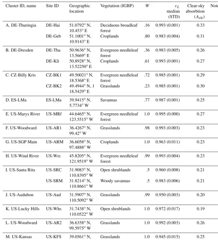
Table 1.List of ground validation targets detailing geographic location and International Geosphere-Biosphere Programme (IGBP) vegetation type. Local parameters determined for each station are weight (W) in spatial average, longwave emissivity and clear-sky absorption.
Cluster ID, name Site ID Geographic Vegetation (IGBP) W εL Clear-sky Notes
location median absorbtion
(STD) (Aclr)
A. DE-Thuringia DE-Hai 51.0792◦N, Deciduous broadleaf .16 0.993 (0.001) 0.33 ∗ 10.453◦E forest
DE-Geb 51.1001◦N, Croplands .80 0.983 (0.004) 0.31 10.9143◦E
B. DE-Dresden DE-Tha 50.9636◦N, Evergreen needleleaf .36 0.983 (0.005) 0.26 13.5669◦E forest
DE-Kli 50.8928◦N, Croplands .61 0.993 (0.001) 0.27 13.52250◦E
C. CZ-Billy Kris CZ-BK1 49.50021◦N, Evergreen needleleaf .72 0.985 (0.001) 0.29 ∗ 18.5368◦E forest
CZ-BK2 49.4944◦N, 1 Grasslands .23 0.985 (0.001) 0.30 18.5429◦E
D. ES-LMa ES-LMa 39.9415◦N, Savannas .77 0.987 (0.001) 0.25 5.7734◦W
E. US-Marys River US-MRf 44.6465◦N, Evergreen needleleaf 1.0 0.995 (0.000) 0.27 123.5515◦W forest
F. US-Woodward US-AR1 36.4267◦N, Grasslands .98 0.993 (0.003) 0.23 99.42◦W
G. US-SGP Main US-ARM 36.6058◦N, Croplands 1.0 0.963 (0.011) 0.23 97.4888◦W
H. US-Wind River US-Wrc 45.8205◦N, Evergreen needleleaf .99 0.993 (0.004) 0.23 121.9519◦W forest
I. US-Santa Rita US-SRC 31.9083◦N, Open shrublands .5 0.960 (0.008) 0.21 110.8395◦W
US-SRM 31.8214◦N, Woody savannas .5 0.983 (0.006) 0.21 110.8661◦W
J. US-Audubon US-Aud 31.5907◦N, Grasslands .99 0.950 (0.003) 0.20 110.5092◦W
K. US-Lucky Hills US-Whs 31.7438◦N, Open shrublands 1.0 0.972 (0.017) 0.19 110.0522◦W
L. US-Woodward US-AR2 36.6358◦N, Grasslands 1.0 0.992 (0.003) 0.26 99.5975◦W
M. US-Kansas US-KFS 39.0561◦N, Grasslands 1.0 0.945 (0.015) 0.25 95.1907◦W
∗Sites are located in neighboring grid cells. Reference: C: Marek et al. (2011).
data (ubRMSE). These three metrics are related as follows:
RMSE=pubRMSE2+bias2. (11)
We further report standard error of estimate (SEE) as a mea-sure of temporal precision:
SEE=σ
q
1−ρ2, (12)
whereσ is the standard deviation of in situ data andρ is Pearson’s correlation coefficient.
3 Results
Table 2.Percentage coverage for two LST products.
MSG domain 2009–2011
Frost-free days
Sat All All All Clear-sky Cloudy
product sky sky
TIR 36 42 47 94 14
MW 50 55 64 75 56
2012. Table 2 lists the amount of days with at least 12 hours of observations for either MW or TIR-LST to give an overall sense of available validation data for this study. In total we have 13 316 data days of in situ data (36 out of 44 data years). Of these data days, 50 % also have MW-LST estimates, and 36 % have TIR-LST observations. For MW, this percentage is negatively affected by the gap between AMSR-E (radiometer turned off in October 2011) and AMSR2 (first observations in July 2012). The MW-LST product is heavily reliant on these satellites with a midday overpass for constraining the diurnal amplitude. For TIR, the percentage is particularly low for GOES due to a more stringent cloud filter than employed for MSG.
To better represent the relative data coverage that is possi-ble with the two LST retrieval techniques, we focus on the four station pairs in the MSG domain and limit the time period to 2009–2011. We further focus on the days where the minimum temperature (as measured at the station) stays above freezing (the MW method is not applicable for sub-freezing temperatures). Within this smaller subset, we have 2506 data days of in situ data, and the coverage of MW is 55 % in comparison with the 42 % coverage for TIR. How-ever, breaking this down by cloud cover reveals the big dif-ference in coverage resulting from the wavelength-dependent tolerance to clouds. During clear skies, the coverage of TIR is 93 %, and MW comes in at 76 % (mainly attributed to the 2-out-of-3-days revisit for ascending AMSR-E). During cloudy days the coverage drops to 13 % for TIR, whereas for MW it maintains 55 % coverage.
In the following section we want to answer two questions. How does the MW-LST compare to TIR-LST in relation to ground data during days with clear skies? And is the perfor-mance of MW-LST affected by clouds? We focus on hourly average temperatures for days where the station data remain above 1◦C to avoid snow or frozen surface conditions. 3.1 Clear-sky comparison of satellite LST products The ground observations provide a common benchmark to test the relative accuracy and bias of the two satellite prod-ucts with the same in situ data. Days with clear skies are selected based on the measure of cloudiness as defined in Sect. 2.3.3, with a maximum accepted value ofAcloud=0.2.
This is in addition to the cloud screening performed in the
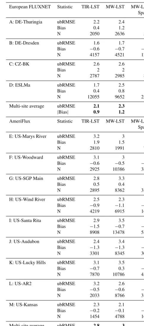
Table 3.Summary of “clear-sky” validation results.
European FLUXNET Statistic TIR-LST MW-LST MW-LST-Sparse
A: DE-Thuringia ubRMSE 2.2 2.4 2.4
Bias 0.4 1.2 1.1
N 2050 2636 525
B: DE-Dresden ubRMSE 1.6 1.7 1.7
Bias −0.6 −0.7 −0.9
N 4157 4521 1245
C: CZ-BK ubRMSE 2.6 2.6 2.6
Bias 2 2 1.9
N 2787 2985 850
D: ESLMa ubRMSE 1.7 2.5 2.6
Bias 0.4 0.8 0.7
N 12055 9652 2560
Multi-site average ubRMSE 2.1 2.3 2.3
|Bias| 0.9 1.2 1.2
AmeriFlux Statistic TIR-LST MW-LST MW-LST-Sparse
E: US-Marys River ubRMSE 3.2 3 3.3
Bias 1.9 1.5 1.7
N 2810 1991 756
F: US-Woodward ubRMSE 3.1 3 2.8
Bias −0.6 −0.5 −0.5
N 2925 10386 3811
G: US-SGP Main ubRMSE 2.8 3.3 3
Bias 0.5 0.4 0.6
N 2895 8362 3105
H: US-Wind River ubRMSE 2.5 2.3 2.5
Bias −0.9 −1.1 −1.1
N 4219 6915 1687
I: US-Santa Rita ubRMSE 2.9 3.5 3.3
Bias −1.5 −0.7 −1.2
N 8908 13478 5312
J: US-Audubon ubRMSE 2.4 3.4 3.4
Bias −1.3 −1.3 −1.6
N 3301 8345 3078
K: US-Lucky Hills ubRMSE 3.1 3.5 3.5
Bias −0.7 0.3 −0.1
N 7870 10786 4545
L: US-AR2 ubRMSE 3.2 2.6 2.4
Bias −0.5 −0.6 −0.6
N 2033 8766 3124
M: US-Kansas ubRMSE 2.3 2.1 2
Bias −0.2 −0.1 −0.4
N 1454 4788 1627
Multi-site average ubRMSE 2.8 3 2.9
|Bias| 0.9 0.7 0.9
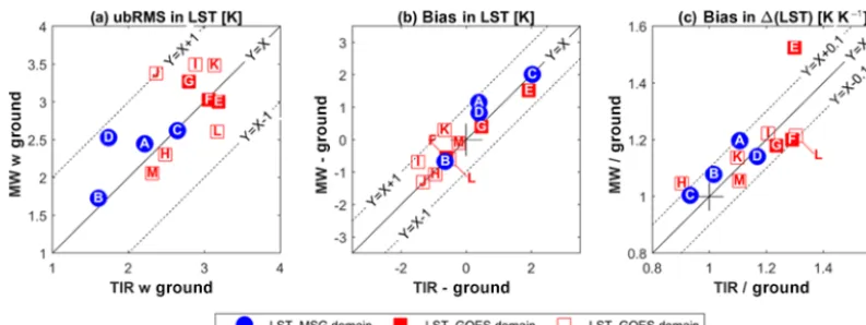
[image:7.612.68.266.85.175.2]Figure 2.Comparison between TIR-LST (xaxis) and MW-LST (yaxis) in terms of their validation metrics with station LST for frost-free and cloud-free days. From left to right the three panels show(a)ubRMSE,(b)mean bias and(c)bias in1(LST). Each marker represents the statistics as calculated for individual locations as identified by the letter (see Table 1 for definition). For the GOES domain the filled markers highlight the stations used in the cloud analysis. Black lines provide visual support and indicate targets (e.g., 1:1 line, cross at zero bias).
the spatial average from the ground stations, they can be used as a reference to compare different satellite LST products.
For each of the 13 validation targets we tabulate (see Ta-ble 3) ubRMSE and bias (see Sect. 2.4 for definition). By ex-cluding long-term bias, the ubRMSE gives an indication of the overall data quality, which includes the random error and errors resulting from a mismatch in variance (either seasonal or diurnal). Errors in spatial representation of the sites affect MW and TIR in the same way. In order to highlight the rel-ative performance of the two satellite products with respect to the common benchmark, we compare their performance directly in Fig. 3.
Encouragingly, the multi-site average ubRMSE for the four European FLUXNET sites shows the MW-LST (2.3 K) to be only moderately higher than TIR-LST (2.1 K) for these frost-free and cloud-free observations. This is a pos-itive result for MW-LST because of the extra processing needed to correct MW data for sensing depth differences with TIR. Both satellite products have a higher ubRMSE with the AmeriFlux stations, but again the multi-site average ubRMSE for MW-LST (3.0 K) is only slightly higher than that for TIR-LST (2.8 K). Figure 2a compares the ubRMSE with in situ data directly for the two satellite technologies. The high correlation between the two methods is an indica-tion that the spurious effect of spatial representaindica-tion of the site affects both methods to similar degrees. Of all the sta-tions, MW-LST has a lower ubRMSE at 5 of the 13 stasta-tions, and the only stations where we record more than 0.5 K differ-ence in ubRMSE between TIR and MW-LST are FLUXNET station D (2.5 K for MW vs. 1.7 K for TIR) and AmeriFlux stations I (3.5 K for MW vs. 2.9 K for TIR) and J (3.4 K for MW vs. 2.4 K for TIR). These stations, together with K and L, all have dry conditions with low vegetation. When there is less vegetation, the influence of soil emissivity on the observed Ka-band brightness temperature becomes larger. Small changes in soil moisture can affect the soil emissivity
and will result in biases for MW-LST when a constant emis-sivity is assumed (as in the current implementation). This points to possible improvements when the scaling to TIR is performed at shorter window lengths, perhaps in 3-month moving windows.
Because MW-LST is scaled directly to TIR-LST, its bias is almost completely determined by the bias between TIR-LST and the site (Table 3 and Fig. 2b). The European FLUXNET sites fall within the MSG domain, and these data years were part of the data on which the scaling of MW-LST is trained (Holmes et al., 2015). Although the mean bias (Fig. 2b) is al-most identical, the bias in morning heating (1T, Fig. 2c) has more variation between the two satellite products. It is inter-esting that generally the satellite products overestimate1T
compared to ground data: on average they both overestimate the recorded heating at the stations by about 10 %.
3.2 Cloud tolerance of satellite LST
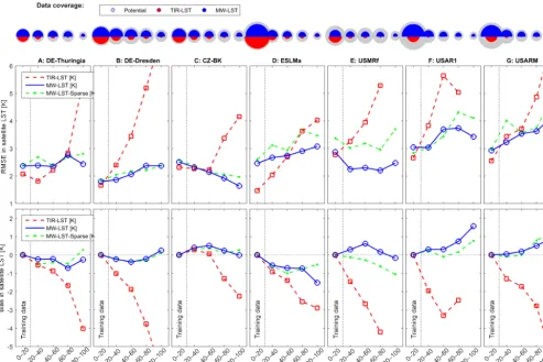
To test the stability of the MW-LST for increasing levels of cloudiness, we took a closer look at the four sites in Eu-rope and three in the US (sites A–G). To isolate the effect of clouds on the agreement between satellite and ground ob-servations, we first remove structural differences by fitting a linear regression for each location, based on data with cloudi-ness below 20 % (0– see Sect. 2c). We then divide the data into five equal bins of increasing cloud coverage from 0 to 100 %. The RMSE and mean difference (bias) between the satellite data and the regression-corrected in situ data is then calculated for each 20 % cloud bin. The purpose is to test the assumption that MW-LST is tolerant to higher levels of cloud coverage.
Figure 3.RMSE and bias of satellite LST with regression-corrected in situ data for five levels of cloud cover ((Acloud, Eqs. 8–10). From left to right are locations A–G (see Table 1 for site information). Results for TIR-LST (red) are contrasted with those for MW (blue). Markers indicate that more than 15 days with data were available for a particular cloud cover bin. Green dashed lines indicate the results for MW-LST-Sparse. For each site and cloud interval the percentage coverage of the temporal record is depicted in the top row with half-rounds in proportion to the number of data pairs. The potential number of data pairs (grey) refers to the number of in situ data points for each cloud bin. The actual number of data pairs is superimposed on this for MW (blue) and TIR (red).
the large increase in negative bias with increasing cloudi-ness for the TIR-LST product stands out. At all stations we see a clear negative bias in response to increasing cloudiness for TIR-LST, and the overall agreement between stations is striking. At 40–60 % cloud cover, all stations but one show a significant negative bias for TIR-LST. Above 60 % cloud cover all stations (where TIR-LST is still available, presum-ably due to failure of the cloud mask) show a negative bias of 2 K or more. This clearly shows that for TIR-LST we have to accept the hypothesis that clouds affect the satellite LST estimate, even after a cloud mask is applied. It is well known that TIR observations are sensitive to clouds and that a fail-ure to mask for cloud conditions will result in an underesti-mated LST (for land surface above freezing). Because of this systematic response to clouds, the bias metric by itself is a good indicator of the effect of cloud contamination in clear-sky TIR-LST products. The symbols in the top row show the diminishing temporal sampling with increasing cloud cover. When we contrast this with the size of the bias, it is clear
that the cloud mask as implemented in the LSA-SAF product (for sites A–D) is not sufficient at removing cloud artifacts. The GOES product (for sites E–G) appears to remove times with high cloud values more completely. Although investi-gating the efficacy of cloud masks for TIR techniques is not the purpose of this paper, it does help illustrate how cloud effects can be identified with these ground stations.
Table 4.Validation results by MW satellite (all data, a.m. or p.m. overpass), aggregated for locations A–M (see Table 1).
2009 linear regression 2015 diurnal scaling
Satellite Overpass RMSE SEE Bias RMSE SEE Bias N
AMSR-E 4.5 3 0.7 3.2 2.6 0.2 6227
a.m. 4.4 1.9 3 3.1 2.1 −1.1 2817
p.m. 4.6 2.7 −1.5 3.3 2.6 1.4 3410
AMSR2 4.4 2.4 1.6 3 1.9 0.8 843
a.m. 5 1.7 3.7 2.6 2 −0.7 347
p.m. 3.8 1.6 −0.3 3.2 1.6 1.9 478
WindSat 3.5 2.3 0.8 3.1 2.5 −0.6 3080
a.m. 3.3 2.1 1.4 3.1 2 −0.2 1617
p.m. 3.7 1.9 0.2 3 2.1 −0.9 1463
SSM/I 3.8 2.4 0.9 3.1 2.6 −0.3 5401
a.m. 3.5 2.3 1.1 3.1 2.2 0.2 2740
p.m. 4 2.1 0.8 3 2.3 −0.8 2661
Average (all sites) 4.1 2.4 1.2 3.1 2.4 0.6
Forest (sites: C, E, H) 5.1 2.1 4.3 3 2 0.5
Low vegetation 3.9 2.5 0.9 3.2 2.5 0.7
The increased retrieval error would still be reflected in an in-creased RMSE. However, the RMSE of MW-LST changes minimally relative to its baseline value at 0–20 % cloudiness and mirrors the size of the bias. This indicates that there is little potential for “hidden” biases behind these numbers. For MW-LST we can therefore reject the hypothesis that clouds affect the satellite LST estimate.
The MW-LST-Sparse product (Eq. 4) adopts the same scaling with TIR as the diurnal MW-LST but has much less sensitivity to the imposed shape of the diurnal model (DTC). For clear skies this distinction is negligible, as apparent from the almost identical values of ubRMSE shown in Table 3. The effect of the clear-sky model is likely to be higher on days with cloudy or partially cloud-covered sky. And although the sparse set only has four–eight observations per day, it allows more samples on days with complex temperature changes. Such days are removed from the MW-DTC product if no good match is found between the diurnal model and obser-vations. We can therefore use the MW-LST-Sparse product to test for undue influence of the DTC model (and its re-lated quality flags) on the relationships between LST errors and cloudiness. The response in bias of MW-LST-Sparse to increasing cloudiness is almost identical to the response of MW-LST for each station (see Fig. 3). In terms of RMSE the sparse set shows values equal to or higher than the diurnally-continuous MW-LST product, which is not surprising as it does not have the smoothing and quality control associated with the DTC model.
3.3 All-sky validation by satellite overpass time
The MW-LST record is a combination of different satellites. In the following analysis the validation results of the MW-LST product are broken down by time of day and satellite in-put record. All data pairs where the minimum temperature at the station stays above freezing are included in this analysis, regardless of cloud cover. It is interesting to compare these results to the much simpler approach that uses a single lin-ear regression model globally (Holmes et al., 2009). Table 4 lists RMSE, SEE and bias for the old and new approach. The statistics are aggregated for all locations as listed in Table 1. The mean scaling with TIR-LST results in a drop in bias for the MW-LST, reducing the average RMSE by 1 K. Part of this reduced RMSE results from the improved characteriza-tion of the amplitude of the diurnal cycle, which improves the slope at all times of day and accounts for 0.2 K of the improvement in RMSE. The impact on the precision (quan-tified here by SEE) is mixed – on average there is no change. Biggest improvements in all metrics are recorded for the for-est locations (sites C, E and H).
4 Discussion
Ka-band (8 mm) is 2 orders of magnitude larger than a typical cloud droplet (10 µm). Therefore, any effect of clouds on MW-LST would stem from changes in associated meteoro-logical conditions like atmospheric vapor content and tem-perature profiles and their potential impact on Ka-band emis-sion processes. According to the zero-order radiative transfer model, an increased atmospheric opacity (through increasing atmospheric water content) increases the weight of the at-mospheric contribution to the satellite-measured brightness temperature, relative to the top of vegetation emission. The sign and size of the effect of a change in atmospheric opacity thus depend on the contrast between the atmospheric tem-perature and the land surface temtem-perature times the effective emissivity. It is therefore possible that this could explain the site-to-site differences in bias as shown in Fig 3. Analyzing the overall effect of the atmosphere on biases in MW-LST will require more detailed atmospheric profile information coupled with a radiative transfer model.
Another possible explanation is that the positive biases recorded at locations F and G are related to scale differences between the site and the 0.25◦grid cell. Spatial heterogeneity in LST is likely more pronounced during clear-sky periods when spatially varying soil and vegetation yield a strong in-fluence on the daytime temperature gradients. During cloudy periods the temperature gradients are not as pronounced and more directly linked to the more uniform air temperature. If the mean temperature at the station is generally higher than the areal mean LST, and this bias diminishes with increasing cloudiness, this would be transformed through our clear-sky training into a positive bias for the satellite product at high cloudiness. However, this effect would affect both MW and TIR to the same extent. We have tested this at locations with two stations in contrasting land cover types (A–C). What we found is that indeed it is possible to “rotate” the bias response by changing the weights of the individual stations and that this rotation affects both MW and TIR-LST. This effect of site representation can therefore explain the greater variation in response from station to station for locations where only one station was available (D–G).
5 Conclusions
In this paper, a recently developed satellite MW-LST product is compared to ground station data and satellite TIR-based LST products. The MW-LST was developed to complement TIR-LST with a coarser spatial resolution but at a higher tem-poral resolution. The higher temtem-poral resolution of MW-LST is based on the assumption that MW has a relatively high tolerance to clouds, which allows for observations at times when no TIR observations are possible. This paper tests this assumption by looking at the precision with respect to ground stations for increasing levels of estimated cloudiness. Our analysis is performed at the 0.25◦spatial resolution as pred-icated by the MW-LST product. At this coarse spatial
res-olution, the overall unbiased RMSE between TIR-LST and ground stations during clear-sky days is 2.1 K for the four lo-cations in the MSG domain, and 2.8 K for the nine lolo-cations in the GOES domain. For the same locations we find that the MW-LST is only slightly higher (+0.2 K for both domains). With increasing cloudiness the RMSE increases signifi-cantly for TIR-LST, caused by a matching negative trend in bias that is seen at all seven locations. This demonstrated the known effect that clouds have on TIR estimates of LST. The fact that these trends are so apparent highlights the lim-itations of current cloud screening techniques as employed in TIR-LST products that are in general use. In clear con-trast to this we find a much more limited response in both RMSE and bias for MW-LST. Because of this we conclude that there is no significant direct impact of clouds on the ac-curacy of the MW-LST product. However, at three stations the size and sign of the response is such that further research is needed to identify the exact causes introducing error in MW-LST. By taking into account the atmospheric humid-ity and temperature profile, further analysis may investigate the extent to which this mixed response can be explained by atmospheric conditions associated with cloudiness. Alterna-tively, if a greater database were available of locations with flux tower sites in contrasting land covers, this could be used to isolate the role of scale mismatch between station and the satellite product.
As an immediate outcome the result of this work high-lights the utility of MW technology for cloud screening of TIR-LST. This is something that will be explored in future work. Ultimately, the goal is to find the best way of combin-ing MW and TIR technology for the estimation of LST from space.
6 Data availability
Acknowledgements. This work was funded by NASA through the research grant “The Science of Terra and Aqua” (13-TERAQ13-0181). We would further like to thank Li Fang (NOAA) for preparation and interpretation of GOES LST.
Edited by: A. Loew
Reviewed by: C. Prigent and one anonymous referee
References
Aires, F., Prigent, C., Rossow, W. B., and Rothstein, M.: A new neural network approach including first guess for re-trieval of atmospheric water vapor, cloud liquid water path, sur-face temperature, and emissivities over land from satellite mi-crowave observations, J. Geophys. Res.-Atmos., 106, 14887– 14907, doi:10.1029/2001JD900085, 2001.
Anderson, M. C., Kustas, W. P., Norman, J. M., Hain, C. R., Mecikalski, J. R., Schultz, L., González-Dugo, M. P., Cammal-leri, C., d’Urso, G., Pimstein, A., and Gao, F.: Mapping daily evapotranspiration at field to continental scales using geostation-ary and polar orbiting satellite imagery, Hydrol. Earth Syst. Sci., 15, 223–239, doi:10.5194/hess-15-223-2011, 2011.
André, C., Ottlé, C., Royer, A., and Maignan, F.: Land surface temperature retrieval over circumpolar Arctic using SSM/I– SSMIS and MODIS data, Remote Sens. Environ., 162, 1–10, doi:10.1016/j.rse.2015.01.028, 2015.
Baldocchi, D., Falge, E., Gu, L. H., Olson, R., Hollinger, D., Running, S., Anthoni, P., Bernhofer, C., Davis, K., Evans, R., Fuentes, J., Goldstein, A., Katul, G., Law, B., Lee, X. H., Malhi, Y., Meyers, T., Munger, W., Oechel, W., U, K., Pilegaard, K., Schmid, H. P., Valentini, R., Verma, S., Vesala, T., Wilson, K., and Wofsy, S.: FLUXNET: A new tool to study the temporal and spatial variability of ecosystem-scale carbon dioxide, water va-por, and energy flux densities, B. Am Meteorol. Soc., 82, 2415– 2434, 2001.
Catherinot, J., Prigent, C., Maurer, R., Papa, F., Jiménez, C., Aires, F., and Rossow, W. B.: Evaluation of “all weather” microwave-derived land surface temperatures with in situ CEOP measurements, J. Geophys. Res.-Atmos., 116, D23105, doi:10.1029/2011JD016439, 2011.
Ermida, S. L., Trigo, I. F., DaCamara, C. C., Göttsche, F. M., Ole-sen, F. S., and Hulley, G.: Validation of remotely sensed sur-face temperature over an oak woodland landscape—The problem of viewing and illumination geometries, Remote Sens. Environ., 148, 16–27, 2014.
Friedl, M. A., Sulla-Menashe, D., Tan, B., Schneider, A., Ra-mankutty, N., Sibley, A., and Huang, X.: MODIS Collection 5 global land cover: Algorithm refinements and characterization of new datasets, Remote Sens. Environ., 114, 168–182, 2010. Göttsche, F.-M., and Olesen, F. S.: Modelling of diurnal
cy-cles of brightness temperature extracted from METEOSAT data, Remote Sens. Environ., 76, 337–348, doi:10.1016/S0034-4257(00)00214-5, 2001.
Göttsche, F.-M., Olesen, F.-S., and Bork-Unkelbach, A.: Validation of land surface temperature derived from MSG/SEVIRI with in situ measurements at Gobabeb, Namibia, Int. J. Remote Sens., 34, 3069–3083, doi:10.1080/01431161.2012.716539, 2013.
Göttsche, F.-M., Olesen, F.-S., Trigo, I. F., Bork-Unkelbach, A. and Martin, M. A.: Long Term Validation of Land Sur-face Temperature Retrieved from MSG/SEVIRI with Contin-uous in-Situ Measurements in Africa, Remote Sens., 8, 410, doi:10.3390/rs8050410, 2016.
Holmes, T. R. H., De Jeu, R. A. M., Owe, M., and Dolman, A. J.: Land surface temperature from Ka band (37 GHz) passive mi-crowave observations, J. Geophys. Res.-Atmos., 114, D04113, doi:10.1029/2008JD010257, 2009.
Holmes, T. R. H., Jackson, T. J., Reichle, R. H., and Basara, J. B.: An assessment of surface soil temperature products from numerical weather prediction models using ground-based measurements, Water Resour. Res., 48, W02531, doi:10.1029/2011WR010538, 2012.
Holmes, T. R. H., Crow, W. T., Yilmaz, M. T., Jackson, T. J., and Basara, J. B.: Enhancing model-based land surface temper-ature estimates using multiplatform microwave observations, J. Geophys. Res.-Atmos., 118, 577–591, doi:10.1002/jgrd.50113, 2013a.
Holmes, T. R. H., Crow, W. T., and Hain, C.: Spatial patterns in timing of the diurnal temperature cycle, Hydrol. Earth Syst. Sci., 17, 3695–3706, doi:10.5194/hess-17-3695-2013, 2013b. Holmes, T. R. H., Crow, W. T., Hain, C. R., Anderson, M., and
Kustas, W. P.: Diurnal temperature cycle as observed by ther-mal infrared and microwave radiometers, Remote Sens. Environ., 158C, 110–125, doi:10.1016/j.rse.2014.10.031, 2015.
Jackson, T. J., Le Vine, D. M., Hsu, A. Y., Oldack, A., Starks, P. J., Swift, C. T., Isham, J. D., and Haken, M.: Soil moisture Map-ping at regional scales using microwave radiometry: The South-ern Great Plains hydrology experiment, IEEE Trans. Geosci. Re-mote Sens., 37, 2136–2149, 1999.
Lei, F., Crow, W. T., Shen, H., Parinussa, R. M., and Holmes, T. R. H.: The Impact of Local Acquisition Time on the Ac-curacy of Microwave Surface Soil Moisture Retrievals over the Contiguous United States, Remote Sens., 7, 13448–13465, doi:10.3390/rs71013448, 2015.
Marek, M. V., Janouš, D., Taufarová, K., Havránková, K., Pavelka, M., Kaplan, V., and Marková, I.: Carbon exchange between ecosystems and atmosphere in the Czech Republic is af-fected by climate factors, Environ. Pollut., 159, 1035–1039, doi:10.1016/j.envpol.2010.11.025, 2011.
Norman, J. M. and Becker, F.: Terminology in thermal infrared re-mote sensing of natural surfaces, Agr. Forest Meteorol., 77, 153– 166, doi:10.1016/0168-1923(95)02259-Z, 1995.
Owe, M. and Van de Griend, A. A.: On the relationship be-tween thermodynamic surface temperature and high-frequency (37 GHz) vertically polarized brightness temperature under semiarid conditions, Int. J. Remote Sens., 22, 3521–3532, doi:10.1080/01431160110063788, 2001.
Owe, M., De Jeu, R. A. M., and Holmes, T. R. H.: Multi-sensor historical climatology of satellite-derived global land surface moisture, J. Geophys. Res.-Earth, 113, F01002, doi:10.1029/2007JF000769, 2008.
Prigent, C., Jimenez, C., and Aires, F.: Towards “all weather”, long record, and real-time land surface temperature retrievals from microwave satellite observations, J. Geophys. Res.-Atmos., 121, 5699–5717, doi:10.1002/2015JD024402, 2016.