Trojans in Wireless Sensor Networks

(1)

Georgia State University Georgia State University

ScholarWorks @ Georgia State University

Mathematics Theses Department of Mathematics and Statistics

Spring 5-10-2014

Influence Function-based Empirical Likelihood Inferences for

Lorenz Curve

Bing Liu

Georgia State University

Follow this and additional works at: https://scholarworks.gsu.edu/math_theses

Recommended Citation Recommended Citation

Liu, Bing, "Influence Function-based Empirical Likelihood Inferences for Lorenz Curve." Thesis, Georgia State University, 2014.

https://scholarworks.gsu.edu/math_theses/136

(2)

INFLUENCE FUNCTION-BASED EMPIRICAL LIKELIHOOD INFERENCES FOR LORENZ CURVE

by

BING LIU

Under the Direction of Dr. Gengsheng Qin

ABSTRACT

In this thesis, an empirical likelihood method based on influence function is developed

and used to construct confidence intervals for the Lorenz ordinates. This method is defined

under the simple random sampling and the limiting distribution of the proposed empirical

likelihood ratio statistic is a standard Chi-square distribution. Extensive simulation studies

are conducted to evaluate the proposed empirical likelihood-based confidence intervals for

the Lorenz ordinates. Finally, this method is used on a real income data as an application.

(3)

by

BING LIU

A Thesis Submitted in Partial Fulfillment of the Requirements for the Degree of

Master of Science

in the College of Arts and Sciences Georgia State University

(4)

Copyright by Bing Liu

(5)

by

BING LIU

Committee Chair: Dr. Gengsheng Qin

Committee: Dr. Xin Qi Dr. Ruiyan Luo

Electronic Version Approved:

(6)

iv

DEDICATION

(7)

v

ACKNOWLEDGEMENTS

This thesis work would not have been possible without the support of many people. First, I want to express my gratitude to my advisor Dr. Gengsheng Qin, who gave me lots of suggestions and guidance while I was doing this thesis research. His insight and knowledge always inspired me and gave me strength when I faced a new challenge.

Furthermore, I want to thank my dear parents and my relatives who always support me once I make my decision to do something. This power is big enough to keep me carrying on. I love you all!

What’s more, my gratitude also goes to our Chair Dr. Guantao Chen, who offered me advice and help. To Dr. Xin Qi and Dr. Ruiyan Luo, my committee members who gave me advice on this thesis. To my undergraduate advisor, Dr. Danhui Yi, who led me into the field of statistics and gave me opportunities to practice while learning new stuff in different views and solving real problems using statistical tools. To Dr. Yichuan Zhao, who gave wonderful lectures on different topics on statistics and biostatistics from which I benefit a lot.

Last but not least, I would like to thank my friends who helped me when I faced diffi-culties while I finished writing this thesis. The friends include but not limited to: Chenxue Li, Yanan Yin, Yuan Liu and Jin Zhao.

(8)

vi

TABLE OF CONTENTS

ACKNOWLEDGEMENTS . . . v

LIST OF FIGURES . . . viii

LIST OF TABLES . . . x

LIST OF ABBREVIATIONS . . . xi

CHAPTER 1 INTRODUCTION . . . 1

CHAPTER 2 A REVIEW OF EMPIRICAL LIKELIHOOD FOR THE LORENZ CURVE WITH SIMPLE RANDOM SAMPLE 4 2.1 Empirical Likelihood . . . 4

2.2 Profile Empirical Likelihood . . . 4

CHAPTER 3 INFLUENCE FUNCTION-BASED EMPIRICAL LIKELI-HOOD FOR THE LORENZ CURVE WITH SIMPLE RAN-DOM SAMPLE . . . 6

CHAPTER 4 SIMULATION STUDY . . . 8

CHAPTER 5 A REAL EXAMPLE . . . 10

CHAPTER 6 CONCLUSIONS . . . 12

REFERENCES . . . 13

APPENDICES . . . 15

(9)

vii

Appendix B COVERAGE PROBABILITIES AND AVERAGE

(10)

viii

LIST OF FIGURES

Figure 1.1 Lorenz Curve . . . 2

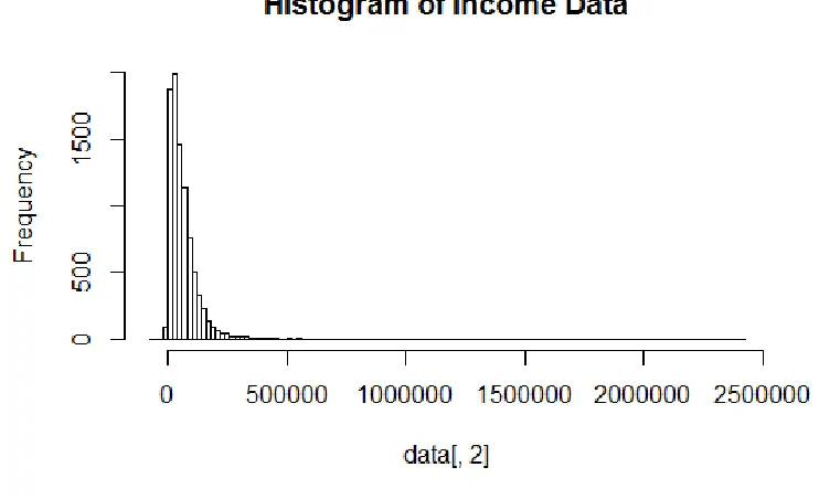
Figure 5.1 Histogram of Income Data . . . 11

Figure A.1 Coverage probabilities of 90% level confidence intervals for Lorenz or-dinates (n=100,Weibull(1,2)) . . . 15

Figure A.7 Coverage probabilities of 90% level confidence intervals for Lorenz or-dinates (n=100,beta(2,5)) . . . 18

(11)

ix

(12)

x

[image:12.612.102.540.129.286.2]

LIST OF TABLES

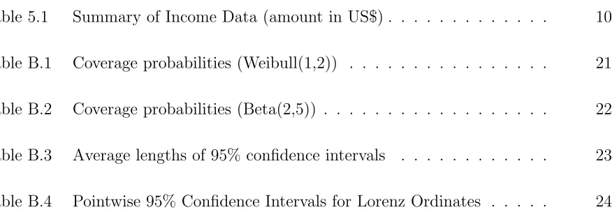
Table 5.1 Summary of Income Data (amount in US$) . . . 10

Table B.1 Coverage probabilities (Weibull(1,2)) . . . 21

Table B.2 Coverage probabilities (Beta(2,5)) . . . 22

Table B.3 Average lengths of 95% confidence intervals . . . 23

(13)

xi

LIST OF ABBREVIATIONS

• GSU - Georgia State University

• EL - Empirical Likelihood

• s.r.s - simple random sampling

• IF - Influence Function

(14)

1

CHAPTER 1

INTRODUCTION

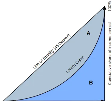
In economics, the Lorenz curve is a graphical representation of income distribution, where it shows the percentage of the total income that the bottom (100*t)% of households have. It was developed by Max O. Lorenz in 1905 [1] for representing inequality of the wealth distribution. If we put the income data in order, the Lorenz curve illustrates the percentage of total income earned by different proportions of the whole population. Let X

be a non-negative random variable with a cumulative distribution functionF(x) and assume thatF(x) is differentiable, Gastwirth (1971)[2] provided a definition of Lorenz curve as below:

η(t) = 1

µ Z ξt

0

xdF(x), t∈[0,1], (1.1)

whereµ=R₀∞xdF(x) is the mean of the distributionF, and ξt =F−1(t) is the t-th quantile

of F. For a fixed t ∈[0,1], the Lorenz ordinate η(t) is the ratio of, the mean income of the lowest t-th fraction of householders, and, the mean income of total householders . Figure 1.1 is a graph describing Lorenz curve [3].

The Lorenz curve has been widely used in different disciplines. In the field of economics and social sciences, it provides a way for the partial ordering of income distributions (Atkin-son, 1970)[4], and analyzing income and earning inequality (Doiron and Barrett, 1996[5]; Sen, 1973[6]). The analysis of Lorenz curve have also been applied in industrial concen-tration (Hart, 1971)[7], reliability (Gail and Gastwirth, 1978)[8], and medical and health services research (Chang and Halfon, 1997[9]; Hallas and Stovring,2006[10]).

However, the income distribution F is rarely known in practice, so we need to estimate the Lorenz curve from the sample income data. LetX1,X2,...,Xnbe an independent sample

(15)

[image:15.612.215.401.76.245.2]

2

Figure 1.1 Lorenz Curve

ˆ

η(t) = 1 ˆ

µ Z ξˆt

0

xdFn(x), (1.2)

where ˆµ is the sample mean, Fn is the empirical distribution function of the sample, ˆξt = inf{y:Fn(y)≥t} is the t-th sample quantile.

Beach and Davison (1983)[11] has developed the asymptotic theory for ˆη. However, the existing normal approximation-based inferential methods have poor performance when the population distribution F is skewed and t falls in the tails of the Lorenz curve.

(16)

3

(17)

4

CHAPTER 2

A REVIEW OF EMPIRICAL LIKELIHOOD FOR THE LORENZ CURVE

WITH SIMPLE RANDOM SAMPLE

2.1 Empirical Likelihood

Let (X1, ..., Xn) be a simple random sample from the population of X with cumulative

distribution functionF. For a fixed t ∈(0,1), the Lorenz ordinate η(t) satisfies:

E[X(I(X ≤ηt)−η(t))] = 0. (2.1)

Thus, the empirical likelihood for η(t) can be defined as:

˜

L1(η(t)) = sup p

( _n Y

i=1

pi : n X

i=1

pi = 1, n X

i−1

piDi(t) = 0 )

, (2.2)

where p= (p1, ..., pn) is a probability vector, Di(t) =Xi[I(Xi ≤ξt)−η(t)], i= 1, ..., n.

2.2 Profile Empirical Likelihood

After substituting ˆξt = X[nt], the t-th quantile estimated from sample, we have the

profile empirical likelihood for η(t):

L1(η(t)) = sup p

( _n Y

i=1

pi : n X

i=1

pi = 1, n X

i−1

piDˆi(t) = 0 )

, (2.3)

where ˆDi(t) =Xi[I(Xi ≤ξˆt)−η(t)], i= 1, ..., n.

A unique maximum forpexists ifη(t) is inside the convex hull ofnX1[I(X1 ≤ξˆt)−η(t)], ... , Xn[I(Xn ≤ξˆt)−η(t)]

o

(18)

5

pi = _n1 n

1 +ν(t) ˆDi(t) o−1

,i= 1, ..., n, whereν(t) is the solution to:

1 n n X i=1 ˆ

Di(t)

1 +ν(t) ˆDi(t)

= 0. (2.4)

So the profile empirical likelihood ratio for η(t) can be defined as:

R1(η(t)) = n Y

i=1

(npi) = n Y

i=1

{1 +ν(t) ˆDi(t)}−1. (2.5)

And the corresponding profile empirical log-likelihood ratio for η(t) is:

l1(η(t)) =−2logR1(η(t)) = 2 n X

i=1

log{1 +ν(t) ˆDi(t)}. (2.6)

We have the following theorem from Qin et al (2013)[18].

T heorem 2.1IfE(X2₎_<_{∞, and}_η₍_t

0) = E[XI(X≤ξt0)]/E(X) for a givent=t0 ∈(0,1),

then the limiting distribution of l1(η(t0)) is a scaled Chi-square distribution with degree of

freedom 1. That is,

r1l1(η(t0))→L χ21,

r1 =s2p(t0)/s2d(t0),

s2 p(t0) =

R∞

0 {x[I(x≤ξt0)−η(t0)]}

2_dF₍_x_),

s2_d(t0) =

R∞

0 {(x−ξt0)[I(x≤ξt0)−xη(t0)]}

2_dF₍_x₎₋₍_t 0ξt0)

2_.

(19)

6

CHAPTER 3

INFLUENCE FUNCTION-BASED EMPIRICAL LIKELIHOOD FOR THE

LORENZ CURVE WITH SIMPLE RANDOM SAMPLE

In the previous chapter, we can see if we want to construct confidence interval for the Lorenz ordinates, we need to find the unknown scale r1, which is complicated. If we take

advantage of the influence function when using empirical likelihood, the limiting distribution of the log-likelihood ratio statistic would be a standard chi-square distribution. Thus, we do not need to estimate the unknown scale. So in this chapter, influence function-based empirical likelihood for the Lorenz curve with simple random sample is introduced.

From results in Qin et al (2013)[18], we can derive:

1

√ n

Pn

i=1Di(t0)

= √1 n

Pn

i=1(Xi[I(X ≤ξt0)−η(t0)])

=√n{1 n

Pn

i=1[(Xi−ξt0)I(Xi ≤ξt0) +t0ξt0 −Xiη(t0)]}+op(1)

=√n{1 n

Pn

i=1g(Xi, η(t0))}+op(1)

where g(Xi, η(t0)) is called the influence function, and

g(Xi, η(t0)) = (Xi−ξt0)I(Xi ≤ξt0) +t0ξt0 −Xiη(t0). (3.1)

Then, based on the estimated influence function ˆg(Xi, η(t0)), where ˆg(Xi, η(t0)) =

(Xi−ξˆt0)I(Xi ≤ξˆt0) +t0ξˆt0 −Xiη(t0), we can define the influence function-based empirical

likelihood for η(t0) as:

LIF(η(t0)) = sup p

( _n Y

i=1

pi : n X

i=1

pi = 1, n X

i−1

piˆg(Xi, η(t0)) = 0

)

. (3.2)

(20)

7

defined as:

RIF(η(t0)) = n Y

i=1

(npi) = n Y

i=1

{1 +νIF(t0)ˆg(Xi, η(t0))}−1, (3.3)

where νIF is the solution to:

1 n n X i=1 ˆ

g(Xi, η(t0))

1 +νIF(t0)ˆg(Xi, η(t0))

= 0. (3.4)

And the corresponding influence function-based empirical log-likelihood ratio forη(t0) is:

lIF(η(t0)) =−2logRIF(η(t0)) = 2 n X

i=1

log{1 +νIF(t0)ˆg(Xi, η(t0))}, (3.5)

Then the following result gives the limiting distribution of the empirical likelihood based on influence function:

T heorem 3.1 If E(X2₎ _< _{∞, and} _η₍_t

0) = E[XI(X ≤ ξt0)]/E(X) for a given t = t0 ∈

(0,1), then the limiting distribution of lIF(η(t0)) is a standard Chi-square distribution, i.e.,

lIF(η(t0))→χ21 as n→ ∞.

(21)

8

CHAPTER 4

SIMULATION STUDY

In this chapter, we’re going to use simulation study to evaluate our method. First, recall the (1−α) confidence interval is defined as RIF ={η(t) : lIF(η(t))≤ χ21,1−α}, equivalently,

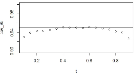
we have p(η(t)∈RIF) = (1−α) +o(1). In the simulation study, the coverage probabilities

and the average lengths of the confidence intervals at different t0s are calculated to evaluate our method.

The coverage probabilities are calculated following these procedures: 1. Generate X1, X2, ... , Xn from a distribution F, n is the sample size.

2. Calculate η(t0) for fixed t0, solve νIF(t0) and get the value of log-likelihood

lIF(η(t0)) =−2logRIF(η(t0)) = 2P_in₌₁log{1 +νIF(t0)ˆg(Xi, η(t0))}.

3. Repeat 1 and 2 for B (a large number) times, then calculate the coverage probability:

1

B B X

b=1

I(η(t0)∈RIF,b) =

1

B B X

b=1

I(lIF,b(η(t0))≤χ21,1−α). (4.1)

At the same time, the average lengths of the 95% confidence intervals are calculated from the generated samples.

When generating samples, we should notice that most income distributions are positively skewed, so the choice of underlying distributionF should be a positively skewed distribution.

Then we choose six different simulation settings as follows:

(22)

9

t= (0.1,0.15,0.2,0.25, ...,0.85,0.9), α= 0.1,α= 0.05

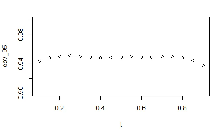
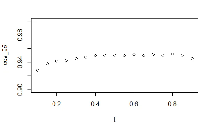
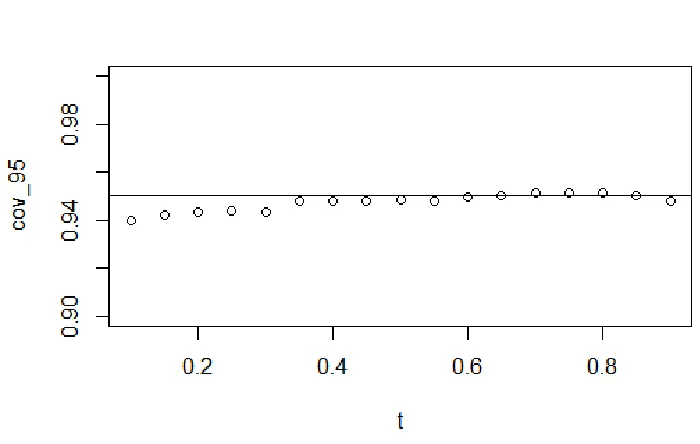
After the simulation, results are shown in the Appendices. In Appendix A, Figure A.1 - Figure A.12 show the coverage probabilities. From these results, we observe that the coverage probabilities of those confidence intervals for Lorenz ordinates are closer to the nominal levels (0.9, 0.95) as sample size increases. Whent0 falls in the lower and upper tails

(23)

10

CHAPTER 5

A REAL EXAMPLE

In this chapter, I apply the influence function-based empirical likelihood method to make inference for Lorenz curve with a real income data.

Income inequality is a significant economic problem. The rising of the inequality is the highest in the United States among most developed countries (Weeks, 2007)[20]. By constructing confidence intervals for Lorenz ordinates at different t, we can discuss how the income inequality is in the United States and have a general view of the inequality.

The income data was selected from the database - The Panel Study of Income Dynamics (PSID) - from the University of Michigan. It is called the 2011 PSID Main Family Data, which contains two variables: 2011 Family Interview (ID) Number and Total Family Income-2010. The income reported here was collected in 2011 about tax year Income-2010. Please note that this variable can contain negative values. Negative values indicate a net loss, which in waves prior to 1994 were bottom-coded at $1, as were zero amounts. These losses occur as a result of business or farm losses. There are in total 8907 households in this dataset.

A brief summary of this income data is shown below:

Table 5.1 Summary of Income Data (amount in US$)

M in. 1stQu. M edian M ean 3rdQu. M ax.

-70000 22620 45880 64870 83000 2420000

(24)

11

[image:24.612.117.488.317.543.2]

but smaller than 0.0116. In other words, the percentage of the income of the lowest 10% households out of the total households is between 0.33% and 1.16%. On the other hand, at t = 0.9, the 95% confidence interval is (0.648726902,0.66399601), so the the ratio of the mean income of the lowest 90% households and the mean income of the total households is greater than 0.6487, but smaller than 0.6640. Similarly, the percentage of the income of the lowest 90% households out of total households is between 64.87% and 66.40%. That means, the top 10% households owned almost 35% percent of the total income in total households in 2010. This is a huge difference between the lower 10% and the upper 10% households, which indicates the severity of the income inequality.

(25)

12

CHAPTER 6

CONCLUSIONS

In this thesis, an empirical likelihood method based on influence function is developed and used to construct confidence intervals for the Lorenz ordinates. This method is defined under the simple random sampling and the limiting distribution of the proposed empirical likelihood ratio statistic is a standard Chi-square distribution. Comparing with the profile empirical likelihood, we get rid of the constant scale which is complicated to calculate.

Simulation results shows good coverage probability and average lengths of the confidence intervals. This interval also has good coverage probabilities even at the lower and upper tail of the Lorenz curve, which gives us a better way to make inferences on Lorenz curve.

The real data example shows the confidence intervals for Lorenz ordinates at different t’s, which give us a general view of the income inequality and how severe it is in the United States.

(26)

13

REFERENCES

[1] M. Lorenz, “Methods of measuring the concentration of wealth,”Journal of the

Amer-ican Statistical Association, vol. 9, pp. 209–219, 1905.

[2] J. Gastwirth, “A general defination of lorenz curve,” Econometrika, vol. 39, pp. 1037– 1039, 1971.

[3] Wikipedia, “Plagiarism — Wikipedia, the free encyclopedia,” 2009, [Online; accessed 14-Feburary-2014]. [Online]. Available: \url{http://en.wikipedia.org/wiki/ File:Economics Gini coefficient2.svg}

[4] A. Atkinson, “On the measurement of inequality,”Journal of Economic Theory, vol. 2, pp. 244–263, 1970.

[5] D. Doiron and G. Barrett, “Inequality in male and female earnings: the roles of hours and earnings,” Review of Economics and Statistics, vol. 78, pp. 410–420, 1996.

[6] A. Sen, On Economic Inequality. New York: Norton, 1973.

[7] P. Hart, “Entropy and other measures of concentration,”Journal of the Royal Statistical

Society: Series A, vol. 134, pp. 73–89, 1971.

[8] M. Gail and J. Gastwirth, “A scale-free goodness-of-fit test for the exponential distribu-tion based on the lorenz curve,”Journal of the American Statistical Association, vol. 73, pp. 229–243, 1978.

[9] R. Chang and N. Halfon, “Graphical distribution of pediatricians in the united states: An analysis of the fifty states and washington, dc,” Pediatrics, vol. 100, pp. 172–179, 1997.

[10] J. Hallas and H. Stovring, “Templates for analysis of individual-level prescription data,”

(27)

14

[11] C. Beach and R. Davison, “Distribution-free statistical inference with lorenz curves and income shares,” Review of Economic Studies, vol. 50, pp. 723–735, 1983.

[12] A. Owen, “Empirical likelihood ratio confidence intervals for single functional,”

Biometrika, vol. 75, pp. 237–249, 1988.

[13] A. B. Owen, “Empirical likelihood ratio confidence regions,” The Annals of Statistics, vol. 18, pp. 90–120, 1990.

[14] P. Hall and B. L. Scala, “Methodology and algorithms of empirical likelihood,”

Inter-national Statistical Review, vol. 58, pp. 109–127, 1990.

[15] J. Chen and J. Qin, “Empirical likelihood estimation for finite populations and the effective usage of auxiliary information,” Biometrika, vol. 80, pp. 107–116, 1993.

[16] X. Zhou, G. Qin, H. Lin, and G. Li, “Inferences in censored cost regression models with empirical likelihood,” Statistica Sinica, vol. 16, pp. 1213–1232, 2006.

[17] S. Chen and J. Qin, “Empirical likelihood-based confidence intervals data with possible zero observations,” Statistics Probability Letters, vol. 65, pp. 29–37, 2003.

[18] G. Qin, B. Yang, and N. E. Belinga-Hall, “Empirical likelihood-based inferences for the lorenz curve,”Annals of the Institute of Statistical Mathematics, vol. 65, no. 1, pp. 1–21, 2013.

[19] M. Zheng, Z. Zhao, and W. Yu, “Empirical likelihood methods based on influence functions,”Statistics and Its Interface, vol. 5, pp. 355–366, 2012.

[20] J. Weeks, “Inequality trends in some developed oecd countries,” United Nations DESA

(28)

15

Appendix A

[image:28.612.191.407.214.334.2]

FIGURES FOR SIMULATION STUDY

[image:28.612.192.407.457.575.2]

Figure A.1 Coverage probabilities of 90% level confidence intervals for Lorenz ordinates (n=100,Weibull(1,2))

(29)

[image:29.612.122.469.133.327.2]

16

[image:29.612.120.470.433.652.2]

(30)

[image:30.612.122.469.133.328.2]

17

[image:30.612.120.469.439.655.2]

(31)

[image:31.612.123.473.135.328.2]

18

Figure A.7 Coverage probabilities of 90% level confidence intervals for Lorenz ordinates (n=100,beta(2,5))

[image:31.612.119.470.435.656.2]

(32)

[image:32.612.122.473.135.328.2]

19

[image:32.612.119.469.434.656.2]

(33)

[image:33.612.124.473.133.326.2]

20

[image:33.612.123.467.450.655.2]

(34)

21

Appendix B

COVERAGE PROBABILITIES AND AVERAGE LENGTHS OF

[image:34.612.145.464.229.519.2]

CONFIDENCE INTERVALS

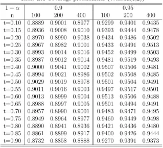
Table B.1 Coverage probabilities (Weibull(1,2))

1−α 0.9 0.95

n 100 200 400 100 200 400

(35)

[image:35.612.146.464.91.378.2]

22

Table B.2 Coverage probabilities (Beta(2,5))

1−α 0.9 0.95

n 100 200 400 100 200 400

(36)

[image:36.612.88.522.96.377.2]

23

Table B.3 Average lengths of 95% confidence intervals

Distn. W eibull Beta

n 100 200 400 100 200 400

(37)

[image:37.612.212.400.95.377.2]

24

Table B.4 Pointwise 95% Confidence Intervals for Lorenz Ordinates