Faint optically selected AGN at z=3

(1)

Thesis by Matthew Philip Hunt

In Partial Fulfillment of the Requirements for the Degree of

Doctor of Philosophy

California Institute of Technology Pasadena, California

2004

(2)

c

2004 Matthew Philip Hunt

(3)

(4)

Acknowledgements

First and foremost, I would like like to thank my advisor, Chuck Steidel, without whom this thesis would not have been possible. His generosity with his time, ideas, and resources was considerable and essential. My fellow travellers in the group, especially Alice Shapley and Kurt Adelberger, not only contributed to the science of this thesis, but also to my happiness as a graduate student. I don’t know how I would have survived so many nights in so many domes (through blizzards, earthquakes, fires, and aurorae) without their conversation and friendship. It seems like Dawn Erb and Naveen Reddy just joined the group, but it has been a few years and countless observing runs, and I am grateful for their company and input.

This thesis also required the hard work of the staff members at the Keck and Palomar observatories. Rick Burruss, Karl Dunscombe, and Jean Mueller spent more time with me at Palomar than anyone should endure, and their respect for the telescope and its science is revealed in their dedication. Palomar Observatory is one of the most special places I have been privileged to visit. The day crew, night assistants, and Monastery hosts all contribute to the best observing environment I can imagine.

Gwen Porter managed to balance the despair of first-year classes with fun and humor, along with the occasional bottle of beer. Mike Santos was always available for pie or conversation, no matter how many deadlines of his own he had. No topic, from large-scale structure formation to monetary policy to teen movies, escaped his grasp. Bryan Jacoby has been the steadiest, best friend I could ask for. Our constant conversations on topics scientific, political, automotive, and œnological required him to spend months in Australia, where he could actually get some work done.

(5)

Bowl; his humor and humility exceeded even his grasp of arcana.

Andy Connolly not only provided data essential to this thesis, and helped with its calibration, but also taught me that Peruvian food is available in Pittsburgh. Max Pettini shared not only his scientific understanding, but his knowledge of the Canary Islands and their avifauna. Mark Metzger built the Large Format Camera, which was essential to this thesis, and he worked at ridiculous hours of the night to fix problems during my observing runs.

I was not privileged to know Bev Oke, who passed away as I was writing this thesis, but I am greatly indebted to him. All of the spectra used in this thesis were obtained with his instruments, the Double Spectrograph and LRIS.

I would like to thank my committee members, Andrew Blain, Wal Sargent, Sterl Phin-ney, and Nick Scoville, for their constructive suggestions that have improved this thesis. Roger Blandford and George Djorgovski also provided helpful suggestions at the beginning of my projects.

(6)

Abstract

We present the results of two surveys for z _≈ 3 AGN, the Lyman break galaxy (LBG) survey and a new survey based on the same techniques, but over a wider area. These surveys, spanning more than 2 deg2, yield 24 new QSOs, and 17 new narrow-lined AGN. The combined data from these surveys span a range of luminosity that is unprecedented at high redshift, covering 6.5 mag of the faint end of the QSO luminosity function. We find a substantially flatter faint-end slope at high redshift than in the local universe, βl= 1.20,

(7)

List of Figures

1.1 The u′ g′

RI filter set . . . 5

1.2 The LBG photometric criteria . . . 6

2.1 Composite AGN spectra (Types I and II) . . . 23

2.2 Spectrum of HDF–oMD49 . . . 24

2.3 Comparison of LBG and Type II AGN spectra . . . 25

3.1 The UV luminosity density of QSOs . . . 37

3.2 Photometric selection function for simulated QSOs . . . 38

3.3 The effective volume of the LBG survey . . . 39

3.4 The QSO LF from the LBG survey . . . 40

4.1 The colors of QSOs from the medium luminosity survey . . . 47

4.2 The effective volume of the medium luminosity survey . . . 50

4.3 The QSO LF from the medium-deep survey . . . 52

4.4 The QSO LF from both surveys . . . 53

5.1 Map of the LFC plate scale . . . 60

5.2 Example parameters: ccdproc . . . 65

5.3 Example parameters: zerocombine . . . 66

5.4 Example parameters: mscsplit . . . 66

5.5 Example parameters: mscsetwcs . . . 69

5.6 Example parameters: msccmatch . . . 69

5.7 IRAF script for merging masks before mscimage . . . 77

5.8 Example parameters: mscimage . . . 78

5.9 Example parameters: imsurfit . . . 79

(10)

5.11 Example parameters: combine . . . 80

5.12 Example of a stacked LFC image . . . 81

5.13 Example parameters: sregister . . . 82

5.14 Example parameters: wcsctran (rotating solutions) . . . 83

(11)

Chapter 1

Introduction

1.1 Background and motivation

The demographics of z _≈ 3 QSOs have been a popular subject of study for many years. Such work has direct implications for the state of the IGM (due to the UV radiation of QSOs), and also on our understanding of galaxy and SMBH formation. Important, well-characterized surveys, including the work of Schmidt et al. (1995), Boyle et al. (1988, 2000), Kennefick et al. (1995), and Fan et al. (2001b), have contributed to the measurement of the QSO luminosity function (QSO LF) at z _≈ 3. However, all of these surveys have an important limitation: Because of the large distance modulus to z = 3, these surveys only went deep enough to observe the brightest QSOs at that redshift.

As a consequence, until the work described in this thesis, there was little reliable in-formation about the demographics of faint QSOs in the distant universe. Pei (1995) drew together an overview of our knowledge of the QSO LF at all redshifts. He found that a double-power law, like that proposed by Boyle et al. (1988), was a good fit to existing LF data at all redshifts, and that there was no evidence for evolution in the faint-end slope (βl = 1.64)1, bright-end slope (βh = 3.52), or normalization (Φ⋆). The redshift evolution

of the LF could be modeled with pure luminosity evolution (PLE): The luminosity of the power-law break is a function of redshift,Lz(z). The functional form of Lz(z) was a

Gaus-sian in z; clearly, this is not a physically-motivated model, but a successful approximation 1

Unless otherwise specified, an Ωm= 1, ΩΛ= 0,h= 0.5 cosmology is used throughout this thesis. This

(12)

to the data. The expressions describing the Pei (1995) model are as follows:

Φ(L, z) = Φ⋆/Lz

(L/Lz)βl+ (L/Lz)βh

(1.1)

Lz(z) = L⋆(1 +z)−(1+α) exp[−(z−z⋆)2/2σ⋆2] (1.2)

Here,z⋆ = 2.75, which may be considered the redshift of peak QSO activity, andσ⋆= 0.93.

The normalization is log(Φ⋆/Gpc−3) = 2.95 and the luminosity of the power law break

is derived from log(L⋆/L⊙) = 13.03. The typical spectral index of QSOs is taken to be

α =₋0.5, a value which is generally used throughout this thesis. The Pei (1995) fit was obtained from LF data in the rest-frame B band, which was the most common choice at the time. Rest-frame 1450 ˚A magnitudes, in the continuum between Lyman-α and C iv, have largely replacedB magnitudes at high redshift, for ease of measurement in the optical. AB 1450 ˚A magnitudes are generally used throughout this thesis, with other results being transformed to this system as necessary.

There are some important limitations to the Pei (1995) fit, however. First, as described above, data on the faint end of the LF were available only at low redshift. Thus, while a constant βl was able to fit the available data at all redshifts, the high redshift data did

not contribute to this constraint. This thesis offers results that improve our understanding of the faint end at high redshifts. Second, even at the bright end, data were limited to

z.4.5, and offered minimal constraints on the bright-end slope atz&3.5. Since then, we have learned that the bright-end slope is not constant at all redshifts; Fan et al. (2001b) have used Sloan Digital Sky Survey (SDSS) data to demonstrate that βh ≈ 2.5 at z ≈4,

significantly flatter than the slope of 3.52 at lower redshifts.

Why has it taken so long to measure the faint end of QSO LF at high redshift? At first glance, the problem may not seem daunting. At z _≈3, observing a number of QSOs down to g′

or r′

of 24 mag would yield a useful measurement, and such magnitudes are easily reached with modern telescopes and instruments, for both imaging and spectroscopy. The problem is twofold. At the faintest magnitudes, say r′

& 24, QSOs are substantially outnumbered by non-active galaxies at the same redshift, and it is difficult to distinguish between them by photometry2. Thus, a large number of faint candidates must be observed

2

(13)

spectroscopically, and only a small fraction of them will yield the desired prey. A QSO survey conducted in this regime would be very costly in effort and telescope time.

At brighter magnitudes, but still within the faint end of the LF (24 . r′

. 21), the problems are different. Contamination by galaxies is no longer a serious problem. QSOs at these magnitudes are less common than fainter ones, due to the shape of the LF, and contamination from stars may be expected (depending on the details of one’s color selection). This source of contamination is not necessarily excessive or difficult to deal with, as we will discuss later. The biggest problem is simply that QSOs are fairly rare objects, and a survey needs to cover a substantial amount of sky (at least a couple of square degrees). It was only recently that wide-field mosaic CCD imagers, such as the Mosaic camera (Muller et al. 1998) on the KPNO 4-m Mayall Telescope and the Large Format Camera (LFC; Simcoe 2003) on the 5-m Hale Telescope, became available. Instruments like these make such surveys considerably more feasible.

In this thesis, we discuss the sample of QSOs3 _{(as well as narrow-lined AGN) discovered}

in two surveys. The first was the survey for Lyman break galaxies (LBGs; Steidel et al. 2003), which is introduced in_§1.2 and presented in detail in Chapters 2 and 3. The second is a survey specifically targeting medium-luminosity QSOs, which is introduced in_§1.3 and discussed more thoroughly in Chapter 4. In addition to the discussions in their respective chapters, an overview of the survey results, and their implications, is provided in _§1.4. Finally, Chapter 5 presents a method for the efficient reduction of LFC data, which was used for the work in this thesis, and has been widely adopted by the Palomar observing community.

1.2 The LBG survey

In the mid-1990’s, an ambitious survey was undertaken to discover and study a large sample of star-forming galaxies at z_≈3. The survey took advantage of photometric pre-selection made possible by the “Lyman break” in the SED of such galaxies, and we refer to the galaxies as Lyman break galaxies (LBGs), and the survey as the LBG survey. The methodology, which is described more completely by Steidel & Hamilton (1993) and Steidel et al. (2003),

3

(14)

was to image a survey field in three filters, Un, G4, and R, with 4–5 m telescopes. The

bandpasses of these filters, not including atmospheric opacity, are shown in Figure 1.1. The

R filter is a custom filter, which is wider than r′

or i′

, and whose central wavelength is intermediate between them.

The imaging data were used to select candidates for spectroscopic observation, based on the following photometric criteria:

R > 19 (1.3)

R < 25.5 (1.4)

G_{− R} < 1.2 (1.5)

(G_{− R}) + 1 < (Un−G) (1.6)

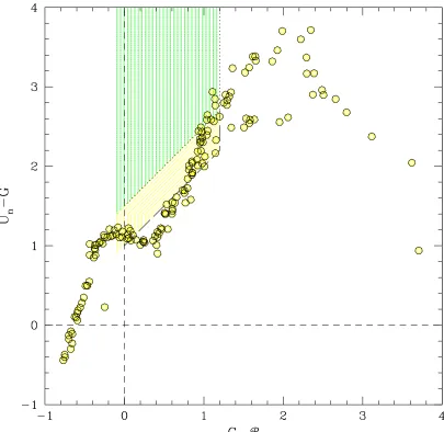
The criterion fundamental to the Lyman break technique, Equation 1.6, selects for objects whose 912 ˚A Lyman break falls between the Un and Gfilters; in other words, at z≈3. A

diagram of the selection window in color space is shown in Figure 1.2.

Whether due to the intrinsic SED, or the substantial opacity of the IGM atz_≈3, QSOs at that redshift also show a Lyman break in their spectra, and hence are included in the photometric selection process as well. They are, in a sense, a “contaminant” in the survey for normal star-forming galaxies, albeit a very small one. At its completion, the LBG survey covered 0.38 deg2 in 17 fields. 2,347 objects met the photometric criteria listed above, and 1,320 of those (56%) were observed spectroscopically at the W. M. Keck Observatory using the Low Resolution Imaging Spectrometer (LRIS; Oke et al. 1995). Of those, 957 (72%) objects were identified as galaxies at z >2. Twelve of those5 _{(1.2%) were QSOs. Another}

16 objects were identified as NL AGN.

It is clear that such a survey, taking hundreds of hours on large telescopes, would not have been undertaken for the sole purpose of finding a dozen faint QSOs. But the LBG survey, having been devised and executed for other purposes, provides us with an unprecedented collection of faint, distant QSOs combined with a readily characterized survey methodology.

4

UnandGare essentially identical to the more recentu′andg′filters. The names are used interchangeably

in this thesis, generally reflecting the “official” names of the filters used in particular observations.

5

(15)

[image:15.612.120.520.158.555.2]

Figure 1.1 Theu′ g′

RI filter set used for the surveys described in this thesis. Theu′

andg′

filters are essentially identical to theUnand Gfilters referred to in certain LBG survey

(16)

[image:16.612.114.519.163.557.2]

Figure 1.2 The LBG photometric selection criteria, in (Un−G,G− R) color space. The

(17)

1.3 The medium-luminosity QSO survey

The LBG survey magnitude limit (_R = 25.5; M1450 ≈ −20) is several magnitudes fainter

than the other surveys mentioned in _§1.1. In fact, when the notion of measuring the LF from these QSOs arose, it was realized that there would be a range of QSO luminosities whose statistics still would not be well constrained. The LBG data would place the first constraints on the very faint end of the LF, to about 6 mag fainter than Lz(z = 3), and

previous work already constrained the bright end [L& Lz(z = 3)]. But in between, from

perhapsM1450 =−23 to−25, it was not expected (based on the assumed shape of the LF)

that the 0.38 deg2 LBG data would contain enough QSOs to strongly constrain the LF. This part of the LF, near the power-law break, is perhaps the most important. With a fairly flat faint-end slope, and steep bright-end slope, a great deal of the total luminosity comes from QSOs just to the faint side of the break. Since we are interested in the QSO contribution to the metagalactic UV radiation field, and QSOs’ effect on the IGM, a good understanding of the integrated LF is essential.

It was therefore decided to conduct a QSO survey essentially identical to the LBG survey, but to shallower depth (_R = 23 instead of 25.5) and over a larger area (about 2 deg2). The photometric criteria (Equations 1.3, 1.5–1.6) would be nearly the same, with some adjustments (borne of experience) to exclude stellar contaminants. Since the selection criteria were the same as the LBG survey, the new “medium luminosity” survey wasn’t restricted to QSOs per se, but based on the magnitude distributions of QSOs, LBGs, and NL AGN from the LBG survey, QSOs were expected to strongly outnumber the otherz_≈3 objects.

It follows naturally from the photometric criteria that the u′

imaging data must be substantially deeper than theg′

or_R data. Furthermore, reaching a certain magnitude in

u′

takes considerably longer than reaching the same magnitude in the other filters. Thus, the

u′

imaging would largely determine the amount of telescope time required to meet the goals stated above. Realizing that a considerable amount of time would be required, we sought a collaboration with A. Connolly, who had already obtained (for another project) sufficiently deepU imaging, in several large fields, using the KPNO Mosaic camera. Combining these data with new g′

(18)

Following the imaging and photometric candidate selection, candidates were observed spectroscopically with the Double Spectrograph (Oke & Gunn 1982) on the Hale Telescope, in various low-resolution configurations. 13 QSOs atz_≈3 were identified by their spectra (as was a single NL AGN), and were merged with the LBG survey QSOs to produce a well-characterized data sample offering good statistics over 6.5 mag in luminosity.

1.4 Results and conclusions from the QSO surveys

The primary result from these surveys was the first measurement of the faint end of the QSO LF at high redshift. A plot of the LF is shown in Figure 4.4 (page 53), along with data points from other surveys. The unexpected finding is that the faint-end slope is substantially flatter at z _≈ 3 than in the local universe, βl = 1.20, compared to 1.64. (The details of

the fit are described in_§3.4 and_§4.3.3.) The integrated LF produces only 50% of the total luminosity predicted by earlier work (e.g., Pei 1995).

Scaling the results of Haardt & Madau (1996), this fit for the LF produces an H i

photoionization rate of ΓH I≈ 8.0×10−13 s−1, which can account for a metagalactic flux

of J912 ≈2.4×10−22 erg s−1 cm−2 Hz−1 sr−1. The constraints on the ionizing flux from

“proximity effect” analyses of the Lyα forest are uncertain, but are consistent with the integrated QSO value at z _≈ 3 (e.g., Scott et al. 2002). In any case, the ratio of the total non-ionizing UV luminosity density of star forming galaxies relative to that of QSOs at z _≈ 3 implies that QSOs must have a luminosity-weighted Lyman continuum escape fraction that is approximately 10 times higher than that of galaxies if they are to dominate the ionizing photon budget.

At shorter wavelengths, like those required to ionize Heii, there is essentially no galactic contribution. Instead, QSOs are the primary source of radiation for the reionization of Heii, which is known to occur atz_≈3 (Jakobsen et al. 1994). As we discuss in detail in_§4.4, the improved measurement of the faint end slope helps to explain several interesting aspects of HeiiLyman-αforest observations, including the strong fluctuations in Heiicolumn density relative to Hi(e.g., Shull et al. 2004).

(19)

that massive SMBHs form earlier than low-mass holes. This prediction is supported by recent observational evidence that even at very high redshifts, luminous QSOs have already formed massive SMBHs. For example, Vestergaard (2004) notes that in luminous z & 4 QSOs, primarily from SDSS, central black holes of 109 _M

⊙ are already present. The author

also remarks that, based on their average spectrum (Figure 2.1), the QSOs discovered in the LBG survey have central black hole masses of&108_M

⊙. If the host galaxies of these QSOs

are essentially LBGs, such large SMBH masses suggest that the black holes are fully-formed before the host galaxies.

Similarly, Wyithe & Loeb (2003) use the local SMBH mass function, in conjunction with a feedback model for SMBH accretion in QSOs, to predict the accretion histories of SMBHs. Their model predicts that the most massive SMBHs are in place by z _≈ 6, in keeping with the observational results described above. In another paper (Wyithe & Loeb 2002), the authors present a physical model for the QSO LF evolution. This model predicts that the QSO phase is triggered by galaxy mergers, and that the duration of the Eddington accretion phase is determined by the mass ratio of small and final galaxies in the merger. Their model successfully predicts the observed bright-end slope of βh ≈2.5 at z&4 (Fan

et al. 2001b), which is shallower than in the local universe.

Thus, it would appear that theory and observations are in general agreement concerning the most luminous QSOs and the most massive SMBHs. As Small & Blandford (1992) predicted, massive SMBHs appear to form quite early. But just as observations have been scarce regarding the faint end of the QSO LF, so has been the theoretical work. There have been few models or predictions about the faint end thus far. One of the few is again due to Wyithe & Loeb (2003), whose self-regulated growth model predicts a steeper faint-end slope at high redshift; combined with the evolution of the bright-end slope, they predict the “break” to disappear at high redshift. This result, of course, is contrary to the observations presented here, and is discussed in Chapter 4. Their prediction is also contrary to a result from the Great Observatories Origins Deep Survey (GOODS) team (Cristiani et al. 2004); as discussed in _§4.4, they observe a deficiency of faint high-redshift QSOs, suggesting a flatter faint-end slope.

(20)

halting, both the QSO activity and star formation, leading to a correlation between the BH and stellar masses. In this scenario, LBGs are generally in the pre-QSO phase, undergoing strong star formation before QSO feedback begins. Such a prediction is consistent with the observations described above, and also with the results of Hosokawa (2004), who concludes that mostz_≈3 LBGs do not have SMBHs, provided mass accretion is dominant process for SMBH growth. (If mergers and/or direct formation are important compared to accretion, the author cannot rule out SMBHs in most LBGs.)

The relationship between LBGs and QSOs at z_≈3 merits further study. In Chapter 2, we calculate a typical QSO duty cycle of approximately 107 yr by noting the fraction of AGN compared to LBGs in the survey (3%) and the average duration of star forming activity in LBGs. This argument rests on the assumption that LBGs are the host galaxies of QSOs at the same redshift. If LBGs do not undergo a strong AGN phase until later (atz.2.7), and the host galaxies ofz_≈3 QSOs are not LBGs at that time, this assumption does not hold. However, various other predictions for the QSO lifetime from other methods are in good agreement (e.g., Hosokawa 2002; Wyithe & Loeb 2002; Yu & Lu 2004; Grazian et al. 2004), and measurements of the cross-correlation between QSOs and LBGs at z_≈3 (Chapter 2) suggest that both objects formed in similar halos, suggesting a similar evolutionary history between LBGs and QSO host galaxies.

The sample of QSOs and NL AGN from the LBG survey also provides an interesting comparison between UV- and X-ray selected samples. As discussed in _§3.4, UV selection has done a very satisfactory job of identifying z _≈ 3 AGN. Even those X-ray selected objects which do not meet the LBG photometric criteria (Equations 1.3–1.6) are generally just outside the selection window, and have optical spectra which are largely similar to the UV-selected objects. There is no evidence for a distinct, X-ray bright population at high redshift that is fundamentally different from the UV-selected AGN.

(21)

et al. (1995) expression for the optical-to-X-ray slope, αox, we find that the expected soft

X-ray flux of a_R= 25, z= 3 QSO is aboutF0.5−2.0 keV≈2.7×10−17 erg s−1 cm−2, which

is very similar to the on-axis sensitivity limit of the 2 Ms Chandra Deep Field (Alexander et al. 2003). There is considerable scatter inαox, so it is not unexpected that some of our

faint AGN do not have sufficient X-ray flux to be detected byChandra.

(22)

Chapter 2

AGN discovered in the

z

= 3

LBG

survey

2.1 Introduction

(23)

past. Despite their possible importance to the overall AGN demographics, only a handful have been identified to date (e.g., Stern et al. 2002; Norman et al. 2002).

At the same time, a very strong case has been developed in the local universe for a tight correlation between the properties of the stellar populations in bulges and spheroids and the mass of central black holes (e.g., Kormendy & Richstone 1995; Magorrian et al. 1998; Merritt & Ferrarese 2001). The presence of this correlation over a very wide range of mass scale strongly suggests that the formation of the spheroid stellar populations and the central black hole are causally linked. One might then reasonably expect that the era during which the spheroid stars were formed might also be that during which the black holes were most likely to be accreting material from gas-rich environs. The “quasar era” is now known to be rather strongly peaked nearz_≈2.5, declining rapidly at both higher and lower redshifts (e.g., Boyle et al. 2000; Warren et al. 1994; Schmidt et al. 1995; Kennefick et al. 1995; Fan et al. 2001b; Shaver et al. 1999). Since it is now possible to routinely observe star-forming galaxies near the peak of the “quasar era,” there is the opportunity to assess the level of AGN activity that is ongoing as the galaxies are undergoing rapid star formation.

In this paper, we present some initial results on the AGN component of a moderately large spectroscopic survey for galaxies selected by their large unobscured star formation rates at redshifts z_≈3. The survey should contain all but the most heavily obscured star forming galaxies at such redshifts (Adelberger & Steidel 2000), and as we detail below, is well-suited for detecting active accretion power in the same star forming objects because of the selection criteria used and the large number of spectra obtained. For the first time at high redshift, it may be possible to assess the fraction of rapidly star forming galaxies that are simultaneously playing host to significant accretion power. In any case, the survey has uncovered a relatively large number of UV-selected, relatively faint, broad-lined and narrow-lined AGN, whose properties we summarize.

We assume a cosmology with Ωm = 0.3, ΩΛ= 0.7, andh= 0.7 throughout this chapter.

2.2 The AGN sample

2.2.1 General Properties and Sample Definitions

(24)

the color, magnitude, and redshift of objects in the targeted sample (Steidel et al. 1999; Adelberger 2002). Some of the details of the LBG selection function are presented in Stei-del et al. (1999); the AGN described in this paper satisfied precisely the same photometric criteria as the star forming galaxies in the sample. The complete details of the LBG photo-metric and spectroscopic survey are presented by Steidel et al. (2003); here we concentrate on the small sub-sample for which there is spectroscopic evidence for the presence of AGN. At redshifts z _≈ 3, the distinctive colors of Lyman break objects depend largely on properties of the intervening intergalactic medium (IGM) where the mean free path of photons shortward of 912 ˚A in the rest frame is short, resulting in a pronounced drop in flux in the observed Un band even for objects whose spectra do not have intrinsic breaks

at the Lyman limit (e.g., Madau 1995; Steidel & Hamilton 1993). Because objects in the spectroscopic sample were selected without regard to morphology (i.e., no attempt was made to remove point sources from the catalog), we expect that our spectroscopic sample should be at least as complete for objects dominated by non-stellar emission as compared to normal star forming galaxies.

The complete catalog of LBG candidates in the z _≈ 3 survey fields consists of 2440 objects in the apparent magnitude range 19.0 _{≤ R ≤}25.5. Simulations suggest that only about 50% of objects with LBG-like intrinsic colors at z_≈3_±0.3 will be included in our color-selected photometric catalogs due to various sources of incompleteness (Steidel et al. 1999). While we attempted to obtain uniform data in each field, variations in Galactic ex-tinction, seeing, sky brightness, and integration time would require each field to be treated independently in a proper evaluation of completeness. Over the full survey, we spectro-scopically observed a total of 1344 objects (55% of the photometric sample), of which 51 are identified as Galactic stars, 988 are high redshift objects with _hz_i = 2.99_±0.29, and 306 remain unidentified. We classified an object as a broad-lined AGN if its spectrum contained any emission line with FWHM greater than 2000 km s−1_{. Such objects always}

(25)

often detectable N v λ1340 and O vi λ1034. Given the quality of the typical LBG sur-vey spectrum, the narrow C iv emission line would have to exceed equivalent widths of a few angstroms in the rest frame, or line fluxes of _∼2_×10−17 _{erg s}−1 _cm−2_{, to have been}

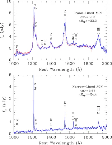
recognized. The coarse properties of the two AGN samples are summarized in Table 2.1. The composite spectra of both classes of AGN, formed by shifting each spectrum into the rest frame based on the emission line redshift, normalizing by the median continuum level in the rest-frame 1600–1800 ˚A range, and averaging, are shown in Figure 2.1. The top panel of Figure 2.1 also shows for comparison the composite spectrum of much brighter QSOs [typically V _∼18, from Sargent et al. (1989) and Stengler-Larrea et al. (1995)] that would satisfy the same LBG color selection criteria. We note the striking similarity of the two QSO samples, which are separated by a factor of about 100 in UV luminosity. There is clear evidence for the Baldwin (1977) effect in the increasing strength of the C ivemission line with decreasing continuum luminosity, and the faint QSO composite has a much more prominent narrow He iiλ1640 emission line.

Our definition of a narrow-lined AGN, based on the detected presence of high ionization emission lines, is admittedly somewhat arbitrary; however, it relies on the fact that the vast majority of LBGs show no detectable emission in Civ and He iieven when Lyman-α

emission is strong, and that it is difficult to produce significant nebular lines of these high ionization species without the hard ionizing spectrum of an AGN component. The line ratios observed among the objects identified as narrow-lined AGN are quite similar to those of local Seyfert 2 galaxies—in fact, for the composite spectrum shown in the bottom panel of Figure 2.1, the Lyα/C iv and Lyα/C iii] ratio are essentially identical to a composite Seyfert 2 spectrum presented by Ferland & Osterbrock (1986). The composite narrow-lined AGN spectrum is also strikingly similar, in both continuum and emission line properties, to the composite spectrum of high redshift radio galaxies from Stern et al. (1999).

(26)

In particular, the spectra of the 2 published “type II” QSOs at high redshift (Stern et al. 2002; Norman et al. 2002) both resemble our faint optically selected narrow-lined AGN spectra in their UV emission line properties. As discussed below, at present there is only limited information on the X-ray emission from objects in the optically selected samples. Clearly, optical/UV selection of AGN will impose different selection criteria than X-ray selection, and there may well be strong X-ray emitting AGN atz >2 that would either not be detected at all in the rest-UV, or not be recognizable as AGN from their UV spectra, because of heavy obscuration. Similarly, because of greater absolute sensitivity in the UV and widely varying UV/X-ray flux ratios (for whatever reason), it may be that faint AGN selection in the UV can identify objects whose X-ray fluxes are still beyond the deepest Chandra integrations. We discuss this issue further in_§2.3.

2.2.2 Estimates of internal completeness of the AGN sub-sample

While a more detailed analysis of the AGN selection function and a derivation of the UV luminosity function of faint AGN are deferred to Chapter 3, here we make some approximate statements on the completeness of our spectroscopic AGN sample. When we could not determine a redshift from a spectrum we had obtained, it was usually due to an absence of emission lines and inadequate continuum signal to measure the relatively weak absorption lines which help establish redshifts for a large fraction of our galaxy sample. Since every AGN in our sample has several strong emission lines (including strong Lyman-αemission), it is unlikely that an AGN with UV-detectable features in the target redshift range would not have been recognized even in spectra of much lower than average quality. We can estimate an upper limit on the number of unrecognized narrow-lined AGN (for reasons of inadequate S/N in the spectra) among those objects identified as normal star-forming galaxies by examining high S/N composite spectra of the LBGs (with identified AGN excluded). The average intensity of C iv emission in the narrow-lined AGN sample is about 20% that of Lyman-α(see Figure 2.1). If we assume that this ratio is characteristic of narrow-lined AGN that we failed to flag as such, and we use the fact that the intensity ratio of Lyman-α to Civemission in the spectral composite of non-AGN LBGs is >

∼100 for the quartile of the

LBG sample having the strongest Lyman-α emission strength1, then an upper limit on the 1

(27)

fraction of AGN-like spectra to have contributed to that sub-sample is_∼5/100 = 5%. The corresponding limit on the fractional contribution of unrecognized AGN to the full LBG sample would then be _∼ 0.25_×5 _≃ 1%. The true fraction with unrecognized AGN-like spectra is likely to be smaller than this limit, since in most individual spectra we could have recognized C iv emission at the level seen in the composite AGN spectrum, and because low-level C iv emission (part of which is due to the stellar P-cygni feature) is expected in the rapidly star forming galaxies even without AGN excitation.

Thus, we expect that, with respect to the photometric LBG sample, the spectroscopic AGN sample is close to Nobs,spec/Nphot = 1344/2440 ∼55% complete, i.e., that any AGN

in the LBG photometric sample that was attempted spectroscopically would have yielded a redshift. We estimate that our present spectroscopic AGN sample contains only_∼30% of the AGN in our fields with 2.7 <

∼z∼< 3.3 and satisfying our photometric criteria R ≤25.5,

G_−R<1.2, andUn−G >(G−R)+1 (i.e., the spectroscopic completeness of 0.55 times the

estimated photometric completeness of_∼50%). The mean redshift of the narrow-lined AGN in our sample is somewhat different from that of the galaxies, probably due to a combination of the subtleties of how the emission lines have affected the broad-band photometry and the redder continuum color (see below). The broad-lined AGN completeness within the photometric sample is expected to be smaller than that of galaxies at a given redshift and apparent magnitude because, at z _≈ 3, only about 60% of (bright) QSO spectra have intervening optically thick Lyman limit systems at high enough redshift to produce the distinctive UV color that we depend on to identify them (Sargent et al. 1989). Galaxies do not suffer this form of incompleteness because they are expected to have significant intrinsic Lyman limits from a combination of stellar spectral energy distributions and opacity to their own Lyman continuum radiation from the interstellar medium2. Again, a careful treatment of these effects is deferred to Chapter 3, but this additional source of incompleteness for broad-lined AGN is likely to be of roughly the same order as the spectroscopic advantage which AGN enjoy when they are observed.

With these caveats in mind, a reasonable estimate of the fraction of AGN among objects in our LBG sample is approximately the same as the fraction of AGN within the

spectroscop-2

We cannot rule out the possibility that faint broad-lined AGN are subject to increased internal Lyman continuum opacity compared to the bright QSOs that have been studied to date; however, the absence of detectable interstellar absorption lines in the composite broad-lined QSO spectrum does suggest that the typical Hicolumn density within the host galaxies along our line of sight is significantly smaller than that

(28)

ically confirmed sample: 29/988, or _∼3%. This number would increase to _∼4% allowing for the maximal incompleteness of the narrow-lined sample discussed above. The observed ratio of narrow-lined to broad-lined AGN, N(NL)/N(BL) = 1.2_±0.4, is consistent with the ratio of broad-lined and narrow-lined radio-loud AGN found by Willott et al. (2001), although we emphasize that our numbers are not yet corrected for relative incompleteness.

2.3 X-ray properties of optically faint AGN at

z

_∼

3

At present, there is only a small amount of information on the X-ray properties of the optically faint AGN in our sample. A cross-correlation of our LBG survey with the 1 Ms exposure of the Chandra Deep Field North (the HDF North region) yields X-ray detec-tions for 4 of the 148 candidates3 (_∼ 3%) in an 8.7′

×8.7′

field centered on the deep HST pointing (Nandra et al. 2002). Of these, two have not yet been observed spectro-scopically. The other two are a faint broad-lined AGN with _R = 24.15 and z = 3.406 (HDF–oC34=J123633.4+621418), and a narrow-lined AGN with _R= 24.84 andz= 2.643 (HDF-MMD12=J123719.9+620955). Both of these AGN have rest-frame 2–10 keV lumi-nosities (uncorrected for intrinsic absorption) of _∼ 5_×1043 _{erg s}−1_{. Our spectroscopic}

Lyman break galaxy sample also contains a clear narrow-lined AGN spectrum, shown in Figure 2.2, that is undetected in the deepChandraimage and thus has an unobscured X-ray luminosity of _∼< 5_×1042 erg s−1 _{in the 2–10 keV band. Thus, while we expect that a large}

fraction of the optically faint AGN in our sample would be detected in the deepestChandra exposures, there is likely also to be a sub-sample that is relatively X-ray faint that would not be detected in even the deepest X-ray pointings to date. Given the overall completeness estimate of _∼30% discussed above, we expect _∼ 20 optically faint (21._R .25.5) AGN (of which_∼11 would be broad-lined objects) over a redshift interval of ∆z_≃0.6 nearz= 3 per 17′

by 17′ _Chandra

ACIS field4. Ostensibly this number is significantly larger than the number of AGN (in a similar redshift range) identified with Chandra sources in the deep fields (e.g., Barger et al. 2001; Hornschemeier et al. 2001; Barger et al. 2001; Stern et al. 2002) although the numbers are small and the follow-up of optically faintChandrasources is still underway. More complete surveys of bothChandrasources and faint optically-selected

3

None of these objects is detected in the radio continuum with the VLA (Nandra et al. 2002)

4

(29)

AGN in the same fields will significantly improve our understanding of the overall AGN demographics at high redshift.

2.4 Are LBGs the hosts of the optically faint AGN?

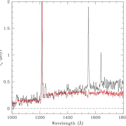
It would be interesting in the context of understanding the history and efficiency of accretion-powered luminosity in galaxies if one could verify that the AGN in the sample are hosted by the equivalent of LBGs5. The range of continuum apparent magnitudes (i.e., the lack of objects brighter than _{R ≈} 23) of the narrow-lined AGN in the spectroscopic sample is similar to that of the non-AGN LBGs in the sample (Table 2.1). The strength of the few interstellar absorption lines that are not strongly masked by emission lines in the composite narrow-lined AGN spectrum are quite similar to those of a composite spectrum of non-AGN LBGs with Lyman-α seen in emission (see Figure 2.3). Unfortunately, the strongest stel-lar feature in the spectra of LBGs is the C iv P-Cygni profile, which is badly affected by Civemission in the composite narrow-lined AGN spectrum. We cannot say with certainty whether the continuum light of the narrow-lined AGN is produced by stellar or non-stellar emission—making this distinction is notoriously difficult even for nearby Seyfert galaxies (e.g., Gonzalez Delgado et al. 1998). However, the far-UV continuum slope (β = ₋0.4, where fλ ∝ λβ) of the composite narrow-lined AGN is redder than all but ∼ 10% of the

LBG sample, and is much redder than the subsample of LBGs with similarly strong

Lyman-α emission, as illustrated in Figure 2.3. If the continuum were attributed to starlight in the same manner as other LBGs then the implied extinction would be a factor of _∼ 50 (Adelberger & Steidel 2000). At this time, only one of the narrow-lined AGN has been observed in the K band, HDF–oMD49 (see Figure 2.2). This object has _{R −}K = 4.20, making it the third-reddest LBG in the observed sample of 118 (Shapley et al. 2001).

The brightest broad-lined object in the sample is more than 2 magnitudes brighter than the brightest narrow-lined object, and there are 5 broad-lined AGN brighter than the brightest narrow-lined AGN. There is some evidence for a flatter magnitude distribution for the broad-lined AGN than for the narrow-lined AGN, but small number statistics and numerous possible selection effects prevent us from making too much of this trend at this time. The relative absence of very UV-bright narrow-lined AGN is at least qualitatively

5

(30)

consistent with the possibility that much of the AGN-produced UV continuum is obscured. There is considerable overlap between our survey fields and planned deep surveys with the Spitzer Space Telescope(SST), so that it should soon be possible to measure many of these optically selected AGN at mid-IR wavelengths, where any bolometrically luminous obscured AGN are expected to be quite prominent.

Assuming that the broad-lined AGN are the less-obscured versions of similar AGN activity, let us suppose for the sake of argument that the mass of putative LBG black holes scales with stellar bulge mass according to the relation established locally, MBH ≈

2_×10−3 _M

bulge (e.g., Ho 1999). Adopting the range of inferred stellar masses of LBGs in

our survey from Shapley et al. (2001), we expect typical black hole masses of 3_×107 _M ⊙

and a range from 2_×106 to perhaps 2_×108 M⊙. If these black holes were radiating at the

Eddington limit, they would be expected to have observed6 ₂₀_.₀ _._R_.₂₄_._{7, close to the}

observed range (for the broad-lined AGN) of 20.6._R.24.8. Apparently, LBGs would be capable of hosting broad-lined AGN with the range of observed UV luminosities.

A more quantitative test of whether the AGN and the LBGs share the same host dark matter halos comes from an evaluation of the clustering statistics of the AGN with respect to LBGs. We have performed tests, using methods similar to those outlined by Adelberger (2002), of the density of LBGs around AGN as compared to that of other (non-AGN) LBGs. Evaluated on scales δz = 0.0085 and δθ = 200 arcmin, we find that the density of LBGs in the vicinity of narrow-lined AGN is 0.96_±0.24 times the density of LBGs around other LBGs. The density of LBGs around broad-lined AGN is 1.58_±0.33 times higher than the density of LBGs around other LBGs. These crude tests suggest that the narrow-lined AGN cluster very similarly to non-AGN LBGs, and that broad-lined AGN may be more strongly clustered than typical LBGs.

In any case, it seems plausible that the observed AGN may be hosted by the equivalent of LBGs. If this is indeed the case, the fraction of LBGs in which obvious AGN activity is present may provide a rough timescale for near-Eddington accretion rates onto central black holes, as follows. The characteristic timescale for star formation episodes in LBGs is estimated to be _∼ 300 Myr, inferred from the modeling of the far-UV to optical (rest-frame) colors (Shapley et al. 2001; Papovich et al. 2001). If the 3% AGN activity reflects

6

Here we assume a radiative efficiency of ǫ∼0.1 for the accretion and that νLν(U V) is a reasonable

(31)

the duty cycle of significant black hole accretion in LBGs, it would imply an active accretion timescale of _∼107 _{years, broadly consistent with the expected black hole masses given the}

implied Eddington mass accretion rate of _∼1 M⊙ yr−1. AGN lifetimes of this order have

been inferred from theoretical studies of black hole growth based on mergers in hierarchical models of structure formation (e.g., Kauffmann & Haehnelt 2000) and from consideration of the QSO luminosity functions and the distribution of black hole masses in the local universe (e.g., Haehnelt et al. 1998; Yu & Tremaine 2002). Significantly longer accretion timescales of _∼ 500 Myr have been suggested by Barger et al. (2001) based on the observation that

∼4% of “L⋆ galaxies at all redshifts” are X-ray sources, but such timescales may refer to

a very different, more protracted process of sub-Eddington accretion onto black holes in well-formed galaxies primarily atz <1.

2.5 Discussion

While we defer more quantitative statements to a future chapter, there are several state-ments we can make that are unlikely to change after more careful modeling of incomplete-ness. First, narrow-lined AGN that are identifiable optically using LBG color selection criteria are quite common, with a space density (at z _≈ 3) 50 to 100 times larger than that of the spectroscopically similar high redshift radio galaxies (cf. Willott et al. 2001). The implied surface density of AGN per square degree per unit redshift at z _≈ 3 reaches approximately 400. It is still uncertain, due to small number statistics and incomplete surveys, what fraction of this number would also beChandra sources that may contribute significantly to the X-ray background7. Nevertheless, we can say with some confidence that narrow-lined AGN make a negligible contribution to the z _≈3 UV background: the total 1500 ˚A luminosity of narrow-lined AGN in our sample is only _∼20% that contributed by the broad-lined AGN, and less than about 2% of that contributed by non-AGN LBGs. We do not know the narrow-lined AGN contribution to the ionizingUV background, but it is likely to be far smaller than 20% of the broad-lined AGN background judging by the red continuum colors and the expectation that the objects are fairly heavily obscured.

Using currently accepted parameterizations of the z_≈3 QSO luminosity function (Pei 1995), about 75% of the AGN-produced ionizing radiation field would come from QSOs

7

(32)

[image:32.612.186.457.111.197.2]

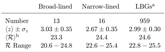
Table 2.1. Properties of the AGN among the z_≈3 LBG sample

Broad-lined Narrow-lined LBGsa

Number 13 16 959

hz_{i ±}σz 3.03±0.35 2.67±0.35 2.99±0.30

hRib 23.3 24.4 24.6

RRange 20.6₋24.8 22.6₋25.4 22.8₋25.5

a_{Excluding objects identified as AGN.}

b_{Mean AB magnitude at an effective wavelength of}

6830 ˚A or_≃1700 ˚A in the rest frame atz_≃3.

that have apparent magnitudes in the range 20.R.25.5, and only about 7% comes from brighter QSOs. Thus, while our sample of broad-lined AGN is fairly small, it extends far deeper than existing QSO surveys8_{, allowing for the first time a direct measurement of the}

AGN contribution to the ionizing radiation field at high redshift. While it is possible that star formation in LBGs may dominate the production of Lyman continuum photons atz_≈3 (Steidel et al. 2001), broad-lined AGN such as those in our faint sample almost certainly provide a substantial fraction of the higher energy photons which apparently reionized Heii

near z _≈ 3. An accurate measurement of the AGN ionizing photon production requires careful attention to issues of photometric and spectroscopic completeness, which will be presented in Chapter 3.

8

The faintest broad-lined AGN in our sample are considerably fainter than the traditional dividing line between QSOs and Seyfert 1 nuclei of MB =−23. This absolute magnitude, for the adopted cosmology,

(33)

[image:33.612.145.505.129.595.2]

(34)

[image:34.612.109.534.225.500.2]

Figure 2.2 The observed spectrum of HDF–oMD49, a type II AGN that is undetected in the 1 MsChandra Deep Field North X-ray image. This object has an unusually weak Lyman-α

(35)

[image:35.612.116.526.158.565.2]

(36)

Chapter 3

Luminosity function from the

z

= 3

LBG survey

3.1 Introduction

The QSO luminosity function (LF) at high redshifts provides important constraints on the ionizing UV radiation field of the early universe. Until now, however, the faint end of the QSO LF has not been measured at high redshift. Instead, low-redshift measurements of the faint end were combined with high-redshift measurements of the bright end to estimate the entire LF at high redshift. Various models of LF evolution have been proposed; for example, a model proposed by Pei (1995) consists of a double power-law (Boyle et al. 1988) whose bright- and faint-end slopes are independent of redshift, and whose power-law break

Lz(z) comes at a luminosity which is proportional to a Gaussian in z, with a maximum

near z⋆ = 2.75 and σ = 0.93 redshift. This model is representative of “pure luminosity

evolution” models, as the overall normalization and the power-law slopes are independent of redshift. While pure luminosity evolution has been shown to work well atz <2.3 (Boyle et al. 1988, 2000), there is now evidence that it is insufficient at high redshift; for example, SDSS results demonstrate that the bright-end slope is flatter at z >3.6 than in the local universe (Fan et al. 2001b). The luminosity of the power-law break and the faint-end slope have not been measured at high redshifts prior to the survey presented here.

(37)

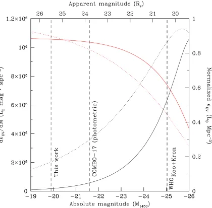
redshift, using a sample of 11 faint z _∼ 3 QSOs discovered in a survey for Lyman break galaxies. Figure 3.1 illustrates the depth of this survey relative to previous z = 3 QSO surveys and demonstrates that the vast majority of the total QSO UV luminosity arises from QSOs bright enough to be included in this survey.

Throughout this paper, the term “QSO” is used to describe all broad-lined AGN without imposing the traditional MB <−23 luminosity cutoff. Spectral properties of such objects

are essentially the same across at least two decades of luminosity (Chapter 2), thus we find no reason to impose such a cutoff. In Section 3.2, we will present an overview of the survey parameters and photometric criteria for candidate selection. In Section 3.3, we will describe our measurements of photometric and spectroscopic completeness, and our calculation of the survey effective volume. The QSO luminosity function will be presented in Section 3.4, followed by a discussion of its implications for the UV radiation field in Section 3.5.

3.2 Survey information

The Lyman break technique has proved to be a successful and efficient means of photomet-rically identifying star-forming galaxies and AGN at z = 3 (Steidel et al. 2003). Similar multicolor approaches have been used in previous, shallower surveys for high-redshift QSOs with good success (e.g. Koo et al. 1986; Warren et al. 1991; Kennefick et al. 1995). Survey fields were imaged in Un (effective wavelength 3550 ˚A), G (4730 ˚A), and R (6830 ˚A)

fil-ters (Steidel & Hamilton 1993). A star-forming galaxy at z = 3 will have a Lyman break in its SED that falls between the Un and Gfilters, resulting in a Un−G color that is

sub-stantially redder than its G_{− R} color. Objects meeting the following photometric criteria were selected as candidatez= 3 galaxies:

R > 19 (3.1)

R < 25.5 (3.2)

G_{− R} < 1.2 (3.3)

G_{− R}+ 1.0 < Un−G (3.4)

(38)

[image:38.612.221.428.137.198.2]

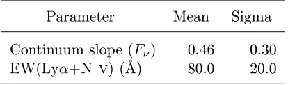
Table 3.1. The mean and sigma of the Gaussian distributions used for simulating the colors of QSOs (see section 3.3.1). TheC iv equivalent width was scaled in proportion to

that of Lyα+N v in order to maintain the template’s original line ratio.

Parameter Mean Sigma

Continuum slope (Fν) 0.46 0.30

EW(Lyα+N v) (˚A) 80.0 20.0

addressed in Section 3.3.

The LBG survey fields used for this study cover 0.43 deg2in 17 fields, which are discussed in detail in Chapter 2). A composite spectrum and other information relating to the 13 QSOs discovered in the survey also appear in Chapter 2. Two of these QSOs satisfied earlier versions of the photometric criteria, but do not satisfy the final versions listed above, and have been excluded from this paper’s results. The sample discussed in this paper, therefore, comprises 11 QSOs.

3.3 Sensitivity to QSOs

3.3.1 Photometric completeness

The intrinsicUn−G andG− R colors of QSOs depend primarily on the spectral index of

their continuum and their Lyman-α+N v equivalent width. To measure the distribution of intrinsic colors (i.e., without the effects of measurement error), we produced a template QSO spectrum consisting of 59 QSOs studied by Sargent et al. (1989, hereafter SSB). These QSOs were discovered using objective prism techniques and are not expected to have significant selection biases in common with multicolor selection techniques. The SSB QSOs are about 100 times brighter than LBG survey QSOs, but a comparison of the SSB and LBG composite spectra suggests that the two populations are sufficiently similar that using the SSB composite as a template is satisfactory (Chapter 2). An average intergalactic absorption spectrum was used to absorption-correct the template using the model of Madau (1995), and portions of the spectrum having poor signal-to-noise were replaced with a power-law fit to the continuum.

(39)

equivalent widths drawn from the Gaussian distributions described in Table 3.1, a compro-mise between the results of Vanden Berk et al. (2001), Fan et al. (2001a), and our SSB template. Each altered spectrum was redshifted to 40 redshifts spanningz= 2.0 toz= 4.0. Intergalactic absorption was added by simulating a random line-of-sight to each QSO with absorbers distributed according to the MC-NH model of Bershady et al. (1999). (For com-parison, an average intergalactic extinction curve (Madau 1995) was also employed. The results were not significantly different.) The spectrum was then multiplied by our filter passbands to produce a distribution of intrinsic colors which reflects the QSO population.

These colors were used to place artificial QSOs into the survey images. 5000 QSOs drawn uniformly from the redshift interval 2.0< z <4.0 and apparent magnitude interval 18.5<

R<26 were simulated in each of the 17 survey fields. The apparent magnitude interval is 0.5 magnitudes larger than the selection window on each end, in order to allow measurement errors to scatter objects into the selection window. The artificial QSOs added to an image were given radial profiles matching the PSF of that image (i.e., they were assumed to be point sources). This assumption has little practical effect, because even galaxies are barely resolved atz= 3, and no morphological criteria were applied to candidates during the LBG survey. The images were processed using the same modified FOCAS (Jarvis & Tyson 1981) software which was used for the actual candidate selection, and the observed colors of the simulated objects were recorded. The intrinsic QSO color distribution was thus transformed to an observed color distribution. Figure 3.2 shows the fraction of simulated QSOs that meet the photometric selection criteria as a function of redshift. As a consistency check, the curve shown was multiplied by R

Φ(L, z) dL to reflect the underlying redshift distribution of QSOs, and compared to the distribution of QSOs discovered in this survey, using a Kolmogorov-Smirnov test. The result wasP = 0.49 using the Pei (1995) LF, andP = 0.45 using the LF shape measured in Section 3.4, indicating consistency between the expected and actual distribution of QSO redshifts.

3.3.2 Spectroscopic completeness

(40)

(_R>23), there were 2,289 candidates in the 17 fields, enough to measure the spectroscopic observation probability as a function of (_R, G_{− R}). The photometric candidates were divided into bins in (_R,G_{− R}) parameter space, using an adaptive bin size which increases resolution where the parameter space is densely filled with candidates. The probability of spectroscopic observation was measured for each bin.

At _R < 23, there are too few photometric candidates to obtain an accurate measure-ment of the selection probability. However, at these apparent magnitudes, candidates with relatively blueG_−Rwere likely to be QSOs and hence were nearly always observed spectro-scopically. Candidates with redG_{− R}were likely to be stellar contaminants, and were less likely to be observed. Hence we have estimated the probability of spectroscopic observation to be unity for candidates with observed magnitudes _R <23 andG_{− R}<1, and 0.5 for candidates with _R < 23 and G_{− R} > 1. The results are insensitive to the latter value because the colors of QSOs are rarely observed to be so red.

We assume that any spectroscopically observed QSO will be identified as such and a redshift obtained, since our spectroscopic integration times were chosen so that we could often identify faint LBGs using their absorption lines (typically 90 minutes using Keck– LRIS). Because QSOs have strong, distinctive emission lines they are easily identifiable even at the faintest apparent magnitudes in the survey (_R= 25.5).

3.3.3 Effective volume of the survey

For comparison with other work, e.g., SDSS, we wish to measure the QSO luminosity func-tion with respect to 1450 ˚A rest frame AB absolute magnitude (M1450). At any given

redshift in this study, we estimated an object’s apparent magnitudem1450 as a linear

com-bination of its _R and G magnitudes. A small redshift-dependent correction, derived from our simulations of QSO colors, was then made to the value. This correction, typically of order 0.25 mag, accounts for Ly-αemission inG, Ly-αforest absorption, and similar effects. If we denote by fphot(m1450, z) the probability that a QSO of apparent 1450 ˚A rest frame

AB magnitudem1450and redshiftzwill have observed colors and magnitudes that meet the

selection criteria for LBGs, and we denote byfspec(m1450, z) the fraction of such candidates

(41)

as a function of absolute magnitude,

Veff(M) =

Z

Ω

Z z=∞

z=0

fphot(m1450(M, z), z) fspec(m1450(M, z), z) dV

dz dΩ dz dΩ (3.5)

where m1450(M1450, z) is the apparent magnitude corresponding to absolute magnitude M1450(R, G, z), Ω is the solid angle of the survey, and dV /dz dΩ is the co-moving

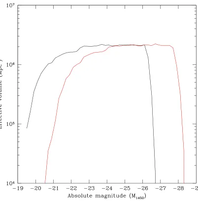
vol-ume element corresponding to a redshift interval dz and solid angle dΩ at a redshift z and using an assumed cosmology. This approach is explained in detail by Adelberger (2002). For this measurement of the LF, we averaged Veff over bins 1 mag in width. The effective

volume of the survey, as a function of absolute magnitude (and in two cosmologies) is shown in Figure 3.3.

3.4 The luminosity function

Having measured the effective volume of the survey as a function of absolute magnitude, we can place points on the QSO luminosity function simply by placing the observed QSOs in absolute magnitude bins and dividing by the effective volume of the survey at that absolute magnitude. A plot of the luminosity function is shown in Figure 3.4. The vertical errorbars indicate 1-sigma confidence intervals reflecting the Poisson statistics due to the number of QSOs in the bin. The uncertainty inVeff is not reflected, as the Poisson statistics dominate

(e.g., there is only 1 QSO in the faintest bin, where imprecisions in photometry lead to the greatest Veff uncertainty). The horizontal errorbars indicate the rms width of the bin,

weighted according to the effective volume and expected luminosity function (Pei 1995) as a function of absolute magnitude; for a bin centered on M = M0 and 1 magnitude wide,

the position of the point and its errorbar width are given by

hM_i =

RM0+1/2

M0−1/2 M Veff(M) Φ(M) dM

RM0+1/2

M0−1/2 Veff(M) Φ(M) dM

(3.6)

σM =

 

RM0+1/2

M0−1/2(M− hMi)

2 _V

eff(M) Φ(M) dM

RM0+1/2

M0−1/2 Veff(M) Φ(M) dM

 

1/2

(3.7)

(42)

precise slope assumed for Φ(M), and retroactively trying our fitted value has no significant effect on the results. An Ωm = 1, ΩΛ = 0, h = 0.5 cosmology has been assumed for

comparison with previous work.

Comparison with the other points shown in Figure 3.4 suggests that our results are largely consistent with previous measurements (Wolf et al. 2003; Warren et al. 1994; Fan et al. 2001b) in the region of overlap. The shape of the LF near the power-law break is somewhat unclear, and our present sample is unable to resolve this issue. The total luminosity of the LF is quite sensitive to the location of the break. A shallower, wide-field survey using identical LBG techniques is nearing completion (Chapter 4), and should better constrain the₋27< M1450 <−24 portion of the luminosity function.

The observed faint-end slope appears to be considerably flatter than βl= 1.64 used by

Pei (1995). The Pei z = 3 LF is shown as the dashed curve in Figure 3.4. In order to quantify the difference, we have fit the double power-law of Boyle et al. (1988), identical in form to that used by Pei,

Φ(L, z) = Φ⋆/Lz (L/Lz)βl+ (L/L

z)βh, (3.8)

whereβlandβh are the faint- and bright-end slopes, respectively,Lz(z) is the luminosity of

the power-law break, and Φ⋆ is the normalization factor. We have combined our data with

those of Warren et al. (1994) to fit the entire luminosity function. The SDSS data plotted in Figure 3.4 were excluded because they were measured atz >3.6, and the authors have demonstrated redshift evolution in the bright-end slope. Given the relatively small number of data points and large errorbars, fits for the four parameters (Lz,Φ⋆, βl, βh) are degenerate.

We have therefore assumed that the Pei (1995) luminosity evolution model still holds, and adopted the same values for Lz and Φ⋆. A weighted least-squares fit for βl and βh was

performed, and the measured faint-end slope was βl = 1.24±0.07. The measured

bright-end slope was βh = 4.56±0.51, but in addition to the large uncertainty, this parameter

is highly degenerate with the assumed parameters Lz and Φ⋆, and is very sensitive to the

brightest data point. Likewise, the errorbars for the faint-end slope are smaller than they would be for a general four-parameter fit. The reduced χ2 _{for the fit is 1.12. This fit for}

the luminosity function is shown as a dashed curve in Figure 3.4.

(43)

completeness at the faint end, by failing to identify the AGN signatures in faint QSOs, perhaps because faint AGN might be overwhelmed by the light from their host galaxies. We do not believe this to be the case, for several reasons. First, in no case have we observed “intermediate” cases of star forming galaxies with broad emission lines superposed. In contrast to virtually all LBG spectra (Shapley et al. 2003), we do not see interstellar absorption lines in any of the spectra of broad-lined objects at z _∼ 3. However, perhaps the strongest argument comes from examining the spectral properties of identifiedz >2.5 X-ray sources in the 2 Ms catalog for the Chandra Deep Field North and other very deep X-ray surveys. If it were common for AGN to be overwhelmed by their host galaxies, there would be a significant number of faint X-ray sources with spectra that resemble those of ordinary star forming galaxies. To date, virtually all published spectra of objects identified in the redshift range of interest have obvious AGN signatures in their spectra, whether they are broad-lined or narrow-lined AGN.

We can also directly compare the Barger et al. (2003) CDF–N catalog with our own color-selected catalog in their region of overlap, with the following results: There are 2 AGN (1 narrow-lined, 1 QSO) which are detected by Chandra and also discovered in the LBG survey; there are 2 QSOs which are detected byChandra but did not have LBG colors in our survey (one of which does have LBG colors in more recent photometry); and there is 1 QSO detected byChandra which has LBG colors but is slightly too faint for inclusion in our survey. These results are consistent with our overall completeness estimates, which are approximately 50% over the range of redshifts considered. In addition, there is a narrow-lined AGN (“HDF–oMD49”) discovered in the LBG survey which is detected in theChandra exposure (Chapter 2) at a level below the limit for inclusion in the main catalog (Alexander et al. 2003); another identified narrow-lined AGN at z = 2.445 has no Chandra-detected counterpart. Of the 84 objects with 2.5_≤z_≤3.5 in our current color-selected spectroscopic sample in the GOODS–N field, only 2 are detected in the 2 MsChandra catalog, and both are obvious broad-lined QSOs.

(44)

3.5 Implications for the UV radiation field at

z

= 3

Having measured the luminosity function of QSOs at z= 3, we can now place constraints on their contribution to the UV radiation field at that redshift. Integrating over the above parametric fit for the QSO luminosity function, in its entirety, yields a specific luminosity density ǫ1450 = 1.5×1025 erg s−1 Hz−1 h Mpc−3. The luminosity density from our

para-metric fit is 50% of that predicted from the Pei (1995) fit (βl = 1.64, βh = 3.52), and is

∼8% of the UV luminosity density produced by LBGs at the same redshift based on the luminosity function of Adelberger & Steidel (2000).

Scaling the results of Haardt & Madau (1996), this fit for the LF produces an H i

photoionization rate of ΓH I≈ 8.0×10−13 s−1, which can account for a metagalactic flux

of J912 ≈ 2.4×10−22 erg s−1 cm−2 Hz−1 sr−1. The ionizing background spectrum and

He ii ionization fraction, which affect this calculation, are the results of models and are discussed in detail by Haardt & Madau (1996). This value should be considered an upper limit, because the ability of ionizing photons produced by faint AGN to escape their host galaxies has not been measured, and may be lower than for the bright QSOs for which self-absorption in the Lyman continuum is rare (see SSB)1_.

The constraints on the ionizing flux from “proximity effect” analyses of the Lyα forest are uncertain, but are still consistent with the integrated QSO value at z _∼ 3 (e.g. Scott et al. 2002). In any case, the ratio of the total non-ionizing UV luminosity density of star forming galaxies relative to that of QSOs at z _∼ 3 implies that QSOs must have a luminosity-weighted Lyman continuum escape fraction that is&10 times higher than that of galaxies if they are to dominate the ionizing photon budget.

The detection of the HeiiGunn–Peterson effect inz_∼3 QSO spectra has demonstrated that helium reionization occurs during this epoch. Unlike the reionization of hydrogen, which can be effected by radiation from both massive stars and QSOs, the reionization of helium requires the hard UV radiation produced only by QSOs. The improved measurement of the faint-end slope, and hence the total UV luminosity density, will improve simulations of the progress of reionization, which have previously assumed the Pei (1995) value for

1

(45)

the faint-end slope (e.g. Sokasian et al. 2002). Miralda-Escud´e et al. (2000) have shown that the previously observed bright end of the luminosity function is sufficient to reionize helium by z= 3 under most reasonable assumptions, so the flatter faint-end slope should not dramatically alter the current picture of He ii reionization; however, our results may have an effect on the “patchiness” of the reionization as it progresses.

A fortunate consequence of the flat faint-end slope, with implications for IGM simula-tions, is that the integrated luminosity R

Φ(L) L dL converges more rapidly, making the integral insensitive to the lower limit of integration. Simulations will therefore be more robust, with less dependence on the poorly understood low-luminosity AGN population at high redshift.

3.6 Conclusions

Using the 11 QSOs discovered in the survey for z _∼ 3 Lyman-break galaxies, we have measured the faint end of the z = 3 QSO luminosity function. This represents the first direct measurement of the faint end at high redshift. While the entire luminosity function remains well-fit by a double power-law, the faint-end slope differs significantly from the low-redshift value of βl = 1.64, being best fit by a slopeβl = 1.24±0.07. This results in only

half the total QSO UV luminosity compared to previous predictions. As measurements of

J912 from the Lyαforest continue to improve, we may find that this diminished luminosity

from QSOs requires a substantial contribution from star-forming galaxies.

(46)

Faint optically selected AGN at z=3

Acknowledgements

Abstract

Contents

List of Figures

Chapter 1

Introduction

1.1

Background and motivation

1.2

The LBG survey

1.3

The medium-luminosity QSO survey

1.4

Results and conclusions from the QSO surveys

Chapter 2

AGN discovered in the

z

= 3

LBG

survey

2.1

Introduction

2.2

The AGN sample

2.3

X-ray properties of optically faint AGN at

z

∼

3

2.4

Are LBGs the hosts of the optically faint AGN?

2.5

Discussion

Chapter 3

Luminosity function from the

z

= 3

LBG survey

3.1

Introduction

3.2

Survey information

3.3

Sensitivity to QSOs

3.4

The luminosity function

3.5

Implications for the UV radiation field at

z

= 3

3.6

Conclusions

_∼