The COsmic ray Soil Moisture Interaction Code (COSMIC) for use in data assimilation

Hydrol. Earth Syst. Sci., 17, 3205–3217, 2013 www.hydrol-earth-syst-sci.net/17/3205/2013/ doi:10.5194/hess-17-3205-2013

© Author(s) 2013. CC Attribution 3.0 License.

EGU Journal Logos (RGB)

Advances in

Geosciences

Open Access

Natural Hazards

and Earth System

Sciences

Annales

Geophysicae

Nonlinear Processes

in Geophysics

Atmospheric

Chemistry

and Physics

Atmospheric

Chemistry

and Physics

Atmospheric

Measurement

Techniques

Atmospheric

Measurement

Techniques

Biogeosciences

Open Access Open Access

Biogeosciences

Discussions

Climate

of the Past

Open Access Open Access

Climate

of the Past

Discussions

Earth System

Dynamics

Open Access Open Access

Earth System

Dynamics

Geoscientific

Instrumentation

Methods and

Data Systems

Open Access

_{Geoscientific}

Instrumentation

Methods and

Data Systems

Geoscientific

Model Development

Open Access Open Access

Geoscientific

Model Development

Hydrology and

Earth System

Sciences

Hydrology and

Earth System

Sciences

Ocean Science

Open Access Open Access

Ocean Science

Discussions

Solid Earth

Open Access Open Access

Solid Earth

Discussions

The Cryosphere

Open Access Open Access

The Cryosphere

Natural Hazards

and Earth System

Sciences

Open Access

Discussions

The COsmic-ray Soil Moisture Interaction Code (COSMIC) for use

in data assimilation

J. Shuttleworth1,2, R. Rosolem1, M. Zreda1, and T. Franz1

1_{Department of Hydrology and Water Resources, University of Arizona, Tucson, USA} 2_{Department of Atmospheric Science, University of Arizona, Tucson, USA}

Correspondence to: J. Shuttleworth ([email protected])

Received: 18 December 2012 – Published in Hydrol. Earth Syst. Sci. Discuss.: 24 January 2013 Revised: 15 June 2013 – Accepted: 1 July 2013 – Published: 14 August 2013

Abstract. Soil moisture status in land surface models

(LSMs) can be updated by assimilating cosmic-ray neutron intensity measured in air above the surface. This requires a fast and accurate model to calculate the neutron inten-sity from the profiles of soil moisture modeled by the LSM. The existing Monte Carlo N-Particle eXtended (MCNPX) model is sufficiently accurate but too slow to be practical in the context of data assimilation. Consequently an alter-native and efficient model is needed which can be calibrated accurately to reproduce the calculations made by MCNPX and used to substitute for MCNPX during data assimilation. This paper describes the construction and calibration of such a model, COsmic-ray Soil Moisture Interaction Code (COS-MIC), which is simple, physically based and analytic, and which, because it runs at least 50 000 times faster than MC-NPX, is appropriate in data assimilation applications. The model includes simple descriptions of (a) degradation of the incoming high-energy neutron flux with soil depth, (b) cre-ation of fast neutrons at each depth in the soil, and (c) scat-tering of the resulting fast neutrons before they reach the soil surface, all of which processes may have parameterized de-pendency on the chemistry and moisture content of the soil. The site-to-site variability in the parameters used in COS-MIC is explored for 42 sample sites in the COsmic-ray Soil Moisture Observing System (COSMOS), and the compar-ative performance of COSMIC relcompar-ative to MCNPX when applied to represent interactions between cosmic-ray neu-trons and moist soil is explored. At an example site in Ari-zona, fast-neutron counts calculated by COSMIC from the average soil moisture profile given by an independent net-work of point measurements in the COSMOS probe foot-print are similar to the fast-neutron intensity measured by

the COSMOS probe. It was demonstrated that, when used within a data assimilation framework to assimilate COS-MOS probe counts into the Noah land surface model at the Santa Rita Experimental Range field site, the calibrated COSMIC model provided an effective mechanism for trans-lating model-calculated soil moisture profiles into above-ground fast-neutron count when applied with two radically different approaches used to remove the bias between data and model.

1 Introduction

Until recently area-average soil moisture at the hectometer horizontal scale has been difficult and costly to measure be-cause of the need to take many point samples, but with the advent of the cosmic-ray method (Zreda et al., 2008, 2012; Desilets et al., 2010) it is now feasible with a single in-strument. However, a complicating aspect of measuring soil moisture using this method is that the volume of soil mea-sured in the vertical varies with soil moisture content (Franz et al., 2012a).

a. diagnose if there is a discrepancy in the modeled soil moisture status from the aboveground measured fast-neutron count; and

b. interpret knowledge of the extent of any discrepancy back into the LSM with weighting between layers re-flecting their relative influence on the aboveground mea-sured fast-neutron count.

This requires the availability and use of an accurate model to interpret the modeled soil moisture profiles in terms of the aboveground fast-neutron count.

In principle the required model needed to make such in-terpretation exists, specifically the Monte Carlo N-Particle

eXtended (MCNPX: Pelowitz, 2005) neutron transport code,

which was much used in establishing the cosmic-ray method (Zreda et al., 2008, 2012; Desilets et al., 2010) currently be-ing deployed in the COsmic-ray Soil Moisture Observbe-ing System (COSMOS: http://cosmos.hwr.arizona.edu/; Shuttle-worth et al., 2010; Zreda et al., 2011, 2012). Given the spec-ified chemistry of the atmosphere and soil (including the amount of hydrogen present as water in the system), the MC-NPX code uses knowledge of nuclear collisions and libraries of nuclear properties for these constituents to track the life history of individual, randomly generated, incoming cosmic rays and their collision products through the atmosphere and in the soil. The code then counts the resulting fast neutrons (we use those in the range 10 eV to 100 eV) that enter a de-fined detector volume above the ground. In principle the MC-NPX code could be used in data assimilation applications to define (a) and (b) in the last paragraph. However, although accurate, the MCNPX code uses the time-consuming Monte

Carlo computational method, and this means its use in data

assimilation applications is impractical.

Therefore an alternative model is needed which can ef-ficiently reproduce the belowground physics, the resulting aboveground count rate and the belowground vertical source distribution of fast neutrons simulated by MCNPX. This paper describes the construction and calibration of such a model, the COsmic-ray Soil Moisture Interaction Code (COSMIC), which is simple, physically based and analytic, and which runs much faster than MCNPX because the nu-clear processes and collision cross sections that are explicitly represented in MCNPX are re-captured in parameters that have dependency on the site-specific soil properties. These parameters are calibrated using multi-parameter optimization techniques against MCNPX calculations for a suite of hypo-thetical soil moisture profiles.

2 Physical processes represented in COSMIC

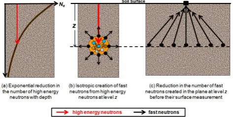
The COSMIC model assumes there are three dominant pro-cesses involved in generating the fast neutrons detected above moist soil (see Fig. 1). It is first assumed that there is an exponential reduction with depth in the number of the

22

Fig. 1. The three physical processes represented in the COSMIC model that are assumed to control the above ground fast neutron count rate. Fig. 1. The three physical processes represented in the COSMIC

model that are assumed to control the aboveground fast-neutron count rate.

high-energy neutrons that are available to create fast neu-trons at any level in the soil. Calculations made with MC-NPX indicate that assuming such an exponential reduction in neutron flux is appropriate. There is reduction due to in-teraction both with the (dry) soil and with the water that is present in the soil. The exponential reduction therefore de-pends on two length constantsL1 andL2, in units of g per

cm2, corresponding to interaction with the soil and the wa-ter (hydrogen), respectively. The mass of wawa-ter includes both

lattice water, i.e., that which is in the mineral grains and

bound chemically with soil and considered fixed in time, and the pore water which is available to support transpiration or drainage and which consequently changes with time. Thus, the number of high-energy neutrons available at depthzin the soil is given by

Nhe(z)=N_he0 exp

−

_m

s(z)

L1

+mw(z)

L2

, (1)

where N_he0 is the number of high-energy neutrons at the soil surface,ms(z)andmw(z)are respectively the integrated

mass per unit area of dry soil and water (in g cm−2)between the depthzand the soil surface, andL1andL2(in g per unit

area) are respectively determined by the chemistry of the soil and its total water content, including any chemically bound lattice water.

Second, it is assumed that at each depthzthe number of fast neutrons created in the soil is proportional to the product of the number of high-energy neutrons available at that depth with the local density of dry soil per unit soil volume and the local density of soil water per unit soil volume at that depth, assuming the relative efficiency of creation of fast neutrons by soil is a factorαof the efficiency of their creation by wa-ter. Consequently, the number of fast neutrons created in the soil in the plane at levelzis given by

Nf(z)=

CN_he0[αρs(z)

+ρw(z)] exp

−

_m

s(z)

L1

+mw(z)

L2

whereC is a (unitless) “fast-neutron creation” constant for pure water,ρs(z)is the local bulk density of dry soil and

ρw(z)the total soil water density, including lattice water. It

is assumed that the direction in which the fast neutrons are generated at levelzis isotropic, i.e., that they leave with equal probability in all directions.

Finally it is assumed that the fraction of fast neutrons orig-inating in the soil in the plane at levelz that are detected above the ground are reduced exponentially by an amount related to the distance traveled between the point of origin in this plane and the detector at the surface. There is then little reduction in the neutron count in the air between the soil surface and the fast-neutron detector mounted just a few meters above the surface. The reduction in fast neutrons in the moist soil is assumed to follow a functional form similar to that in Eq. (1), i.e., an exponential reduction, as for high-energy neutrons, but with different length constantsL3 and

L4, in units of g cm−2, corresponding to attenuation by soil

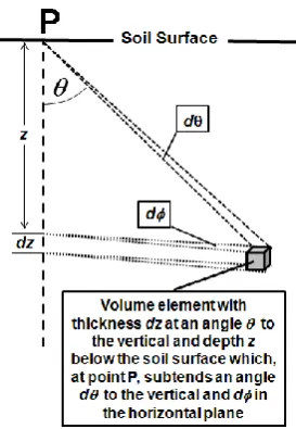
and by (total) soil water, respectively. However, because the direction in which fast neutrons are generated at levelzis as-sumed to be isotropic, fast neutrons reaching the surface will travel further if they do not originate directly below the detec-tor, rather from a point that is more distant in the horizontal plane at levelz. To allow for this it is necessary to calculate the integrated average of the attenuation for all points in this plane to the detector, with the attenuation distance being in-versely proportional to cos (θ ), whereθis the angle between the vertical below the detector and the line between the de-tector and each point in the plane; see Fig. 2. Consequently, the integrated average attenuation of the fast neutrons gener-ated at levelzbefore they reach the detector is given by the functionA(z):

A(z)=

1 2π

Z2π

0 

 

2 π

π/2 Z

0 exp

₋

1 cos(θ )

ms(z)

L3 + mw(z)

L4

·dθ 

 ·dφ, (3) which, because there is assumed symmetry around the verti-cal through the detector, reduces to

A (z)= ₂

π

Zπ/2

0

exp ₋₁

cos(θ )

ms(z)

L3

+mw(z)

L4

·dθ . (4)

The value ofA(z) can be found numerically, but for effi-ciency it could also be adequately calculated using the ap-proach described in Appendix A.

Combining the representations of the three physical pro-cesses considered in COSMIC described above, the analytic function describing NCOSMOS, the number of fast neutrons

reaching the COSMOS probe at a near-surface measurement point is

NCOSMOS=

N ∞ Z

0

A (z)[αρs(z)+ρw(z)] exp

− _m

s(z) L1

+mw(z) L2

·dz.(5)

23

Fig. 2. The source volume element of fast neutrons created in the plane at depth z in the soil which may reach the measurement point P, but whose number is attenuated by an exponential factor with length constants L3 and L4 (in g per unit area), these being respectively determined by the chemistry of the soil and by the total water content of the soil, including lattice water.

Fig. 2. The source volume element of fast neutrons created in the plane at depthzin the soil which may reach the measurement point P but whose number is attenuated by an exponential factor with length constantsL3and L4(in g per unit area) – these being

re-spectively determined by the chemistry of the soil and by the total water content of the soil, including lattice water.

Note that in Eq. (5), the product of the two constants (CN0)

that appears in Eq. (2) has been replaced by a single constant,

N, because the values ofCandN0cannot be separately

de-termined from a comparison between calculations made us-ing COSMIC and MCNPX.

3 Determining the parameters to be used in COSMIC

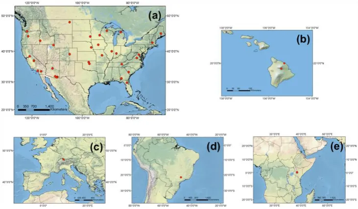
To determine the values of the (in some cases site-specific) parameters to be used in COSMIC, at 42 selected sites in the COSMOS network (see Fig. 3) for which the required data were available at the time of this analysis, simulations us-ing COSMIC were calibrated against equivalent calculations made with the MCNPX model. The MCNPX calculations were made using the site-specific COSMOS probe calibra-tion based on gravimetric samples (see, for example, Franz et al., 2013a, b), corrected for the effect of atmospheric hu-midity (see Rosolem et al., 2013), and with site-specific bulk density of the soil, soil chemistry and lattice water content (see Table 2 in Zreda et al., 2012, for values).

BecauseL2 andL4relate to attenuation by water alone,

their values are independent of the soil chemistry of the site and they can be determined by substituting pure water for dry soil in MCNPX and COSMIC calculations. A simula-tion with MCNPX was made with pure water substituting for soil, and an exponential function then fitted to the cal-culated reduction in high-energy neutrons with depth calcu-lated by MCNPX for pure water to determineL2. The

3208 J. Shuttleworth et al.: The COSMIC for use in data assimilation

24

Fig. 3. The locations of the 42 sites in (a) the continental USA, (b) Hawaii, (c) Europe, (d) South America and (e) Africa for which optimization of the COSMIC model parameters given in Tables 1 were made. (For site details, go to http://cosmos.hwr.arizona.edu/Probes/probemap.php and click on the site of interest.)

Fig. 3. The locations of the 42 sites in (a) the contiguous USA, (b) Hawaii, (c) Europe, (d) South America and (e) Africa for which optimization of the COSMIC model parameters given in Table 1 were made. (For site details, go to http://cosmos.hwr.arizona.edu/Probes/ probemap.php and click on the site of interest.)

the required value of the parameterNfirst defined at this site. This was accomplished by first optimizing the values of all remaining four COSMIC parameters (N,α,L3,L4) at this

site, withL2given as previously discussed andL1computed

directly from MCNPX, in a similar manner to that described below. OnceNis determined, COSMIC is configured to sim-ulate pure water, and the parameterL4is fine-tuned to match

the same neutron count obtained directly from MCNPX at the San Pedro site (after appropriate scaling using theF term described in the last paragraph of this section and shown in Table 1). Notice that for pure water simulations, the terms as-sociated with parametersα,L1, andL3no longer appear in

Eq. (5). Based on these pure water simulation comparisons, the values ofL2andL4were set to 129.1 and 3.16 g cm−2at

all COSMOS sites.

The value ofL1is easily determined for each site by

run-ning MCNPX with dry soil that has the site-specific soil chemistry and then fitting an exponential function to the cal-culated exponential reduction in high-energy neutrons with depth simulated by MCNPX (analogous to the method used to determinedL2described above). Although the value ofL1

may depend on the soil chemistry present, our simulations with MCNPX at the 42 COSMOS sites considered in this study suggest thatL1is only weakly related to soil chemistry,

with site-to-site variability around the mean value for all sites being just∼1 %. On this basis, adopting a fixed value equal to 162.0 g cm−2irrespective of site is a reasonable assump-tion.

Data from individual sites in the COSMOS network are corrected for site to site differences in elevation and cutoff rigidity but local variability remains, likely associated with

site-to-site differences in soil chemistry or vegetation cover. Individual site calibration of sensors is therefore required to allow for the fact that the observed neutron flux intensity at calibration does not necessarily equal the neutron flux inten-sity calculated by MCNPX when run with the soil chemistry and water content observed at calibration; see the final para-graph in Sect. 4. The values of the site-specific constants

N, αandL3 at all sites were then determined using

multi-parameter optimization techniques against calculations made using MCNPX. At each site calculations of the aboveground fast-neutron count are made using MCNPX for the 22 hy-pothetical profiles of volumetric water content illustrated in Fig. 4, i.e., for 10 profiles with different uniform volumet-ric water content, and 12 with different linear gradients of volumetric water content to a depth of 1 m and with uni-form volumetric water content below 1 m. One criterion used in parameter optimization to define the preferred values of

N, α, andL3is the weighted mean absolute error (MAE)

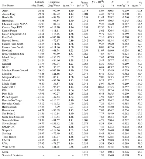
Table 1. Site-specific values of latitude and longitude;ρs(g cm−3),θlattice(m3m−3)andF; and the parametersN, α(cm3g−1)andL3

(g cm−2) obtained by calibrating the COSMIC model against MCNPX at the 42 COSMOS sites shown in Fig. 3 withL1=162.0 g cm−2,

L2=129.1 g cm−2, andL4=3.16 g cm−2.

Latitude Longitude ρs θlattice F(×1014) N α L3

Site Name (deg North) (deg West) (g cm−3) (m3m−3) (–) (–) (cm3g−1) (g cm−2)

ARM-1 36.61 −97.49 1.40 0.075 8.07 510.5 0.239 107.8

Austin Cary 29.74 −82.22 1.42 0.004 4.47 247.3 0.290 110.3

Bondville 40.01 −88.29 1.45 0.058 11.43 708.2 0.240 113.1

Brookings 44.35 −96.84 1.40 0.042 6.97 430.5 0.245 106.1

Chestnut Ridge NOAA 35.93 −84.33 1.41 0.032 9.28 546.0 0.267 108.5

Coastal Sage UCI 33.73 −117.70 1.16 0.051 12.30 745.1 0.272 80.1

Daniel Forest 41.87 −111.51 1.14 0.033 5.62 326.4 0.298 79.1

Desert Chaparral UCI 33.61 −116.45 1.58 0.020 9.79 575.7 0.259 130.1

Fort Peck 48.31 −105.10 1.28 0.049 7.10 429.5 0.270 93.6

Harvard Forest 42.54 −72.17 0.89 0.042 10.59 613.4 0.327 56.0

Hauser Farm North 34.58 −111.86 1.36 0.033 9.27 556.0 0.262 102.3

Hauser Farm South 34.58 −111.86 1.50 0.039 8.05 482.6 0.251 120.5

Howland 45.20 −68.74 1.23 0.059 11.07 669.0 0.254 88.2

Iowa Validation Site 41.98 −93.69 1.53 0.069 7.87 507.1 0.224 124.3

Island Dairy 20.00 −155.29 0.69 0.144 7.63 469.8 0.306 50.0

JERC 31.24 −84.46 1.38 0.011 5.47 297.7 0.302 104.4

Kendall 31.74 −109.94 1.23 0.064 8.30 506.3 0.269 87.3

KLEE 0.28 36.87 1.00 0.058 6.69 413.7 0.285 65.4

Manitou Forest Ground 39.10 −105.10 1.40 0.039 7.17 434.9 0.259 106.9

Metolius 44.45 −121.56 1.04 0.044 6.41 378.3 0.312 69.4

Morgan Monroe 39.32 −86.41 1.38 0.041 9.00 543.5 0.257 105.0

Mozark 38.74 −92.20 1.43 0.053 9.25 557.1 0.252 109.9

Mpala North 0.49 36.87 1.45 0.041 5.99 353.0 0.269 114.0

Neb Field 3 41.16 −96.47 1.42 0.051 10.65 635.5 0.257 109.9

P301 37.07 −119.19 1.06 0.042 5.26 312.6 0.299 70.8

Park Falls 45.95 −90.27 1.26 0.021 6.44 365.5 0.299 90.7

Pe-de-Gigante −21.62 −47.63 1.32 0.022 4.91 278.7 0.290 98.0

Rancho No Tengo 31.74 −110.02 1.40 0.044 6.77 394.2 0.274 107.5

Reynolds Creek 43.12 −116.72 0.90 0.052 7.26 433.4 0.318 57.0

Rietholzbach 47.38 8.99 0.94 0.047 9.22 542.0 0.306 60.9

Rosemount 44.71 −93.09 1.45 0.042 7.05 424.2 0.254 113.6

San Pedro 2 31.56 −110.14 1.40 0.056 7.77 464.9 0.262 107.3

Santa Rita Creosote 31.91 −110.84 1.46 0.037 7.65 463.4 0.251 114.8

Savannah River 33.38 −81.57 1.41 0.008 4.71 260.4 0.292 108.3

Silver Sword 19.77 −155.42 0.78 0.075 8.38 509.1 0.332 50.0

SMAP-OK 36.06 −97.22 1.46 0.076 7.46 475.3 0.232 115.6

Soaproot 37.03 −119.26 1.02 0.041 5.92 346.0 0.310 66.9

Sterling 38.97 −77.49 1.32 0.084 8.45 513.4 0.264 96.5

Tonzi Ranch 38.43 −120.97 1.48 0.076 9.83 628.5 0.232 118.0

UMBS 45.56 −84.71 1.29 0.005 4.74 268.8 0.293 94.4

UVA 37.92 −78.27 1.14 0.035 5.38 320.3 0.289 79.0

Wind River 45.82 −121.95 0.88 0.058 6.66 394.5 0.318 55.5

Mean – – – 0.047 7.67 460.3 0.276 94.0

Standard Deviation – – – 0.025 1.95 124.0 0.028 22.4

by Zreda et al. (2008); i.e., at the site the cumulative contribu-tion has a 2-e folding depth of around 0.76 m for a prescribed uniform volumetric water content of 0 %, and around 0.12 m for a prescribed uniform volumetric water content of 40 %, with zero lattice water content in both cases.

25

Fig. 4. The 22 prescribed profiles of soil water content (10 uniform and 12 with constant gradients) for which calculations of the above ground fast neutron count in the COSMOS detector are made using both MCNPX and COSMIC during parameter estimation.

Fig. 4. The 22 prescribed profiles of soil water content (10 uniform and 12 with constant gradients) for which calculations of the above-ground fast-neutron count in the COSMOS detector are made using both MCNPX and COSMIC during parameter estimation.

of multi-operator search and self-adaptive offspring creation, as well as the implementation of population-based elitism search. The initial parent population of sizen is generated using Latin hypercube sampling (McKay et al. 1979). The fast non-dominated sorting algorithm approach (Deb et al., 2002) is used to assign the Pareto-rank for multiple criteria. Subsequent generation of the offspring (with the same size

n)occurs with the use ofkoperators. The approach adopted in this study, which is similar to that presented by Rosolem et al. (2012), uses a population of sizen=100, and number of operators (search strategies)k=4, and set the maximum number of generations,s=1000, so that the total number of simulations (s×n) is 100 000.

This multi-parameter optimization was made at all 42 sites considered in this study to obtain the site-specific preferred values ofN, α, andL3when the values ofL1,L2andL4are

specified to be 162.0, 129.1 and 3.16 g cm−2_{, respectively.}

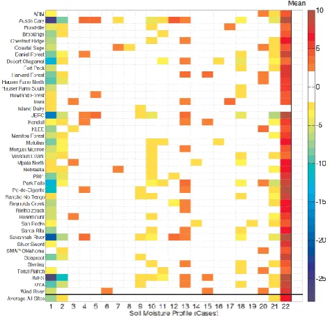
The resulting optimal parameters are given in Table 1 (the factorF given in column four of this table is discussed and used later in Sect. 5). Figure 5 summarizes the overall re-sults of the multi-parameter optimization procedure, given the value of the difference between the simulated neutron count given by COSMIC (with optimized parameters) and the equivalent neutron count scaled from MCNPX, normal-ized by the MCNPX count (represented by colors for each site and each hypothetical soil moisture profile). Because MCNPX is a Monte Carlo model, the neutron count given by MCNPX is subject to random sampling errors of the order 1 %, and this contributes to some of the normalized differ-ences illustrated in Fig. 5. For a substantial majority of the sites and hypothetical soil moisture profiles the normalized difference between the COSMIC- and MCNPX-simulated neutron counts is within the range 2–3 %, and when aver-aged over all sites the normalized difference is much less than this (Fig. 5, bottom row). This range in normalized dif-ference is comparable to the measurement uncertainty in the COSMOS probe and the sampling error in the soil moisture field at probe calibration, including for the drier soil profiles for which the differences are greatest.

26

Fig. 5. Percentage difference illustrated by color (see key to the right) between the simulated neutron count given by COSMIC with optimized parameters and the neutron count given by MCNPX normalized by the MCNPX count for each of the sites shown in Fig. 3 and each of the hypothetical soil moisture profiles shown in Fig. 4. The last column (labeled Mean) shows the site-average difference, while the bottom row shows the average across all sites. For comparison, the typical observation error in a COSMOS probe is around 2%.

Fig. 5. Percentage difference illustrated by color (see key to the right) between the simulated neutron count given by COSMIC with optimized parameters and the neutron count given by MCNPX nor-malized by the MCNPX count for each of the sites shown in Fig. 3 and each of the hypothetical soil moisture profiles shown in Fig. 4. The last column (labeled Mean) shows the site-average difference, while the bottom row shows the average across all sites. For com-parison, the typical observation error in a COSMOS probe is around 2 %.

4 Correlations and dependencies of optimized parameters

It is of interest to investigate the extent to which the site-specific optimized values ofN, αandL3are correlated with

each other and with the site-specific values ofρs, the

aver-age bulk density for the soil in g cm−3, andθlattice, the lattice

water content of the soil in m3m−3. In practice, there is no evidence of correlation between the site-specific value of the parameter N and the site-specific values of ρs, α andL3:

linear correlation of these three parameters withN givesR2

values of 0.01, 0.19, and 0.01, respectively. There is also no evidence of correlation between the site-specific optimized values ofαandN withθlatticeat each site (R2=0.04 and

0.06, respectively), and little evidence of correlation of L3

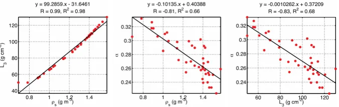
withθlattice(R2=0.30). However as Fig. 6 shows, the

site-specific values ofL3andαboth exhibit evidence of

correla-tion withρs, the bulk density for the soil at each site, and the

site-specific values ofL3andαare also mutually correlated.

ArguablyL3andαare indeed both independently correlated

withρs, but the possibility exists that one of the parameters

(likelyL3)is correlated, and the apparent correlation of the

27

Fig. 6. Correlation of the site-specific optimized values of (a) L3 and (b) with the

site-specific value of s, and (c) correlation between the site-specific optimized values of 

and L3.

Fig. 6. Correlation of the site-specific optimized values of (a)L3and (b)αwith the site-specific value ofρs, and (c) correlation between the

site-specific optimized values ofαandL3.

their influence onNCOSMOScalculated by Eqs. (3) and (5) is

to change its value in opposite directions.

It is worth noting that, in physical terms, a strong cor-relation between L3 and ρs implies the attenuation of fast

neutron by (dry) soil is not well described as an exponen-tial decay with a simple single length constant that is

inde-pendent of the density of soil as assumed in COSMIC.

In-stead the effective value of the length constant appears to be a near-linear function of soil density. Similarly a (true) corre-lation betweenαandρsimplies that the creation of fast

neu-tron from high neuneu-trons is not perfectly described as a linear function of the local density of dry soil; i.e., in Eq. (2) the product [αρs] becomes [0.404(ρs)−0.101(ρs)2]. It is

possi-ble that the observed correlations ofL3andαwithρsmay be

useful for COSMOS sites where a multi-parameter optimiza-tion against MCNPX is not feasible because approximate es-timates ofL3andαmight then be made from measured value

ofρsusing the following equations:

L3= −31.65+99.29ρs (6)

α=0.404−0.101ρs. (7)

The marked variability in the site-specific optimized values of the parameterN must reflect substantial variability in one or both of the component constantsCorN_he0. However, there should be limited variability inN_he0 because the site-specific neutron calculations given by MCNPX against which cali-bration was made were corrected for local station effects us-ing a scalus-ing factor to account for differences in cosmic ray intensity as a result of the elevation/cutoff rigidity of the site where the probe is located (for details see Desilets and Zreda, 2003). The contributing variability is therefore presumably primarily associated with the effective value ofC. This site-to-site variability is intrinsic to the COSMOS array (rather than a feature associated with the COSMIC model) and is present in the site-specific factorF (given in column 4 of Ta-ble 1).F is the ratio between the number of counts observed during COSMOS probe calibration at a specific site and the calculated neutron flux intensity given by MCNPX when run with the soil chemistry and water content (including lattice

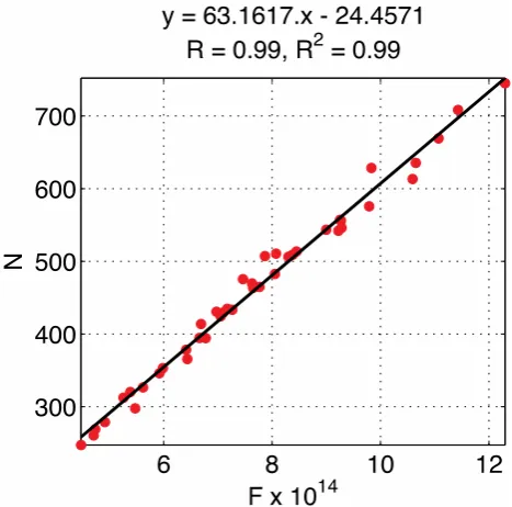
water) observed at each probe site during calibration. (Note: the factor 1014inF arises because MCNPX actually calcu-lates neutron fluence, the time integration of neutron flux, rather than neutron count rate directly.) Figure 7 shows the strong interrelationship between the COSMIC parameterN

found by multi-parameter optimization and the factorF:

N= −24.46+63.16×10−14F. (8)

The origin of the real site-to-site variability inF across the COSMOS array is currently under investigation. It is possi-ble there is some remnant contribution to variability inF as-sociated with the location and altitude of the probe although the neutron count rates were corrected for these (Desilets and Zreda, 2003). It is also possible that differences in the ambi-ent water vapor contambi-ent of the air during probe calibration may make some contribution to the variability in F at the level of a few percent (for details, see Rosolem et al., 2013). Otherwise the variability inF is presumably associated with site-to-site differences in soil chemistry or more likely vege-tation cover (Franz et al., 2013a, b).

5 Application of the COSMOS probe at the Santa Rita study site

28

Fig. 7. Relationship between the COSMIC parameter N found by multi-parameter optimization and the factor F, this being the ratio between the number of counts observed during the COSMOS probe calibration at a specific site and the calculated neutron flux intensity given by MCNPX when run with the soil chemistry and water content (including lattice water) observed at each probe site during calibration.

Fig. 7. Relationship between the COSMIC parameterN found by multi-parameter optimization and the factorF, this being the ratio between the number of counts observed during the COSMOS probe calibration at a specific site and the calculated neutron flux inten-sity given by MCNPX when run with the soil chemistry and water content (including lattice water) observed at each probe site during calibration.

soil moisture calculated from TDT point sensors does not sample the near-surface soil moisture above 10 cm depth and, as a result, does not recognize the faster rate of drying of surface soil moisture. Consequently, when the area-average profile measured by the TDT probes is used in the COSMIC model to calculate the COSMOS probe count, the estimated COSMOS count is underestimated.

As previously stated, the primary purpose of the COSMIC model is to facilitate use of observed COSMOS probe counts into LSMs through ensemble data assimilation methods. We foresee two broad data assimilation applications using COS-MIC, specifically to provide

i. the best estimate of the rate of change in the area-average soil moisture profile when this is being calcu-lated by a prescribed (but perhaps imperfect, e.g., bi-ased) LSM, to obtain improvement in the calculated moisture loss from the surface to the atmosphere, in a Numerical Weather Prediction model for example. Ar-guably in this application the data assimilation process primarily needs to correct for weaknesses in the high-frequency dynamics of the soil moisture profile calcu-lated by the model rather than its absolute value; and ii. the best estimate of the (albeit LSM-calculated)

area-average profile of soil moisture at a COSMOS probe site, this as a basis for investigating and building models

29

Fig. 8. At the Santa Rita Experimental Range field site, (a) the Time-Domain Transmission (TDT) probes installed at one of the soil profiles; (b) the locations at which the paired vertical profiles of TDT probes were installed within the footprint of the COSMOS probe (note the location of the TDT profiles are biased towards making measurements within the 1e-fold area sampled by the COSMOS probe); and (c) comparison between the fast neutron count observed by COSMOS probe (black, with grey to show estimated error), and that calculated using COSMIC (red) and using MCNPX (blue with estimated error) from the area-average soil moisture profile measured with TDT profiles.

Fig. 8. At the Santa Rita Experimental Range field site, (a) the time domain transmission (TDT) probes installed at one of the soil pro-files; (b) the locations at which the paired vertical profiles of TDT probes were installed within the footprint of the COSMOS probe (note the location of the TDT profiles are biased towards making measurements within the 1e-fold area sampled by the COSMOS probe); and (c) comparison between the fast-neutron count observed by COSMOS probe (black, with grey to show estimated error) and that calculated using COSMIC (red) and using MCNPX (blue with estimated error) from the area-average soil moisture profile mea-sured with TDT profiles.

of the relationship between area-average soil moisture and area-average hydro-ecological behavior at the site for example. In this application the data assimilation process primarily needs to correct for weaknesses in the absolute value of the model-calculated profile.

layer. The observational uncertainty in the COSMOS counts is well defined by Poisson statistics and equal to the square root of the sensor hourly count (Zreda et al., 2008), but, given the typical number of counts from an individual COS-MOS probe, this Poisson distribution of the errors can be ad-equately approximated by a Gaussian distribution.

In each of the example cases discussed below the data as-similation is carried out within the National Center for At-mospheric Research (NCAR) Data Assimilation Research Testbed (DART) framework (Anderson et al., 2009), this be-ing a community facility for ensemble data assimilation. The Bayesian framework employed in DART combines the prob-ability distribution of the prior ensemble with the observa-tion likelihood (data distribuobserva-tion) to compute an updated en-semble estimate (posterior distribution) and increments to the prior ensemble. Increments for each component of the prior state vector are computed by linear regression from the in-crements calculated in observation space. We use the ensem-ble adjustment Kalman filter (EAKF) discussed in Ander-son (2001) applied hourly. The updated ensemble is obtained by shifting the prior ensemble to have the same mean as the continuous posterior distribution, and the posterior ensemble standard deviation is kept the same as the continuous poste-rior by linearly contracting the ensemble members around the mean. In this application we used 40 ensemble members with both the meteorological forcing and soil moisture initial con-ditions perturbed following standard procedures as described in the literature (see Table 2). The soil moisture initial con-ditions are perturbed around a reference value determined by the COSMOS sensor with an initial assumed uniform profile (the conversion from neutron counts to integrated soil mois-ture is achieved by applying Eq. A1 in Desilets et al., 2010). Sequential data assimilation was applied via the EAKF to neutron counts, and the soil moisture state variables in Noah updated appropriately every time a new (hourly) observation was available.

Draper et al. (2011) state that when applying data assimi-lation methods, a primary goal is to address the cause of bias between the data and model rather than to rely on data assim-ilation to correct it, while Yilmaz and Crow (2013) also em-phasize that biases should be removed prior to assimilating data. There are several ways to remove such bias (through a priori scaling approaches or through a bias estimation mod-ule, for example); in the context of a paper whose primary purpose is to describe the formulation and calibration of the COSMIC model, we follow Kumar et al. (2012) and choose to demonstrate application of COSMIC when using two rad-ically different alternate approaches for removing relative bias, i.e. first by assuming the bias is solely in the data and “modifying the data to match the model”, and second by as-suming the bias is in the model and “recalibrating the model to match the data”.

In fact there is a large systematic bias between soil mois-ture calculated by the Noah LSM and the value deduced from COSMOS observations at the Santa Rita field site. This

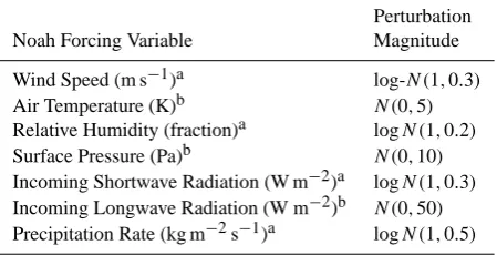
Table 2. List of meteorological forcing variables applied to the Noah model and perturbed during ensemble data assimilation to-gether with the nature of the perturbation applied to them. The perturbation distribution was either log-normal (i.e., multiplying the reference variable) or normal (i.e., adding to or subtracting from a reference value). The magnitude of perturbations used in the DART framework is based on a literature review of several studies including Zhou et al. (2006), Zhang et al. (2010), Reichle et al. (2002, 2007, 2008), Walker and Houser (2004), Sabater et al. (2007), Kumar et al. (2012), Dunne and Entekhabi (2005), Mar-gulis et al. (2002), Reichle and Koster (2004).

Perturbation

Noah Forcing Variable Magnitude

Wind Speed (m s−1)a log-N (1,0.3)

Air Temperature (K)b N (0,5)

Relative Humidity (fraction)a logN (1,0.2)

Surface Pressure (Pa)b N (0,10)

Incoming Shortwave Radiation (W m−2)a logN (1,0.3)

Incoming Longwave Radiation (W m−2)b N (0,50)

Precipitation Rate (kg m−2s−1)a logN (1,0.5)

a_{Multiplicative perturbation;}b_{additive perturbation.}

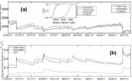
is clearly apparent in the inset graph in the top panel of Fig. 9, which shows that the cumulative distribution func-tion (CDF) of neutron counts computed by COSMIC us-ing soil moisture profiles from an offline simulation of Noah LSM (NOAH-COSMIC, shown in black) has systematically lower values than those observed by both the COSMOS sen-sor (COSMOS-real, shown in blue) and the counts computed with the average soil moisture profile from the TDT network (TDT-derived, shown in purple). Although it is clear that in this particular case the source of bias originates from the in-ability of the model to accurately represent reality, nonethe-less we proceed to demonstrate use of COSMIC when used in the “modifying the data to match the model” approach and apply CDF-matching (Reichle and Koster, 2004; Drusch et al., 2005) to scale the COSMOS observations (COSMOS-scaled, in green) to match the CDF obtained from Noah LSM offline simulation. Figure 9a shows the time series of the re-sulting scaled version of the observed neutron count (green) together with the neutron count (calculated by COSMIC) from the soil moisture profiles simulated by the Noah model when running open loop (black) and with the assimilation of COSMOS data (red). Similarly, Fig. 9b shows the depth-average soil moisture for the Noah model when running open loop (black) and with the assimilation of COSMOS data (red), together with the area-average soil moisture measured by the TDT network (purple). To enhance consistency be-tween these three depth averages they are all weighted by the relative contribution to the aboveground fast-neutron flux for each level (calculated by COSMIC).

30

Fig. 9. Application of the COSMIC model to assimilate COSMOS probe counts into the Noah land surface model at the Santa Rita Range field site. The insert in (a) shows the Cumulative Distribution Function (CDF) of neutron counts measured by the COSMOS probe (COSMOS-real, blue), computed by COSMIC from the measured area-average TDT profile (TDT-derived, shown in purple), computed by COSMIC from soil moisture profiles simulated by the (uncalibrated) Noah LSM, and from the COSMOS observations after they have been scaled by CDF matching (NOAH-COSMOS-scaled, shown in green). (a) Time series of the resulting scaled version of the observed neutron count (green) together with the neutron count (calculated by COSMIC) from the soil moisture profiles simulated by the Noah model when running open loop (black) and with the assimilation of COSMOS data (red). (b) shows the depth-average soil moisture for the Noah model when running open loop (black) and with the assimilation of COSMOS data (red) together with the area-average soil moisture measured by the TDT network (purple). To enhance consistency between the three depth averages in (b) they are all weighted by the relative contribution to the above ground fast neutron flux for each level (calculated by COSMIC).

Fig. 9. Application of the COSMIC model to assimilate COSMOS probe counts into the Noah land surface model at the Santa Rita Range field site. The insert in (a) shows the cumulative distribution function (CDF) of neutron counts measured by the COSMOS probe (COSMOS-real, blue), computed by COSMIC from the measured area-average TDT profile (TDT-derived, shown in purple), com-puted by COSMIC from soil moisture profiles simulated by the (un-calibrated) Noah LSM, and from the COSMOS observations after they have been scaled by CDF matching (NOAH-COSMOS-scaled, shown in green). (a) Time series of the resulting scaled version of the observed neutron count (green) together with the neutron count (calculated by COSMIC) from the soil moisture profiles simulated by the Noah model when running open loop (black) and with the assimilation of COSMOS data (red). Panel (b) shows the depth-average soil moisture for the Noah model when running open loop (black) and with the assimilation of COSMOS data (red) together with the area-average soil moisture measured by the TDT network (purple). To enhance consistency between the three depth averages in (b) they are all weighted by the relative contribution to the above-ground fast-neutron flux for each level (calculated by COSMIC).

sought to eliminate the systematic bias by improving the performance of Noah LSM via a priori parameter calibra-tion. When doing this we again employed the AMALGAM method (see Sect. 3) withn=100, k =4, and s=200 to constrain 10 parameters used in Noah (and each individual layer soil moisture initial condition) which were selected based on a preliminary sensitivity analysis. We found that the values of all ten parameters were changed by calibration to some extent, but four model parameters changed signif-icantly, namely FXEXP, REFKDT, SMCREF, and DKSAT, which control bare-soil evaporation, surface infiltration, on-set of transpiration stress due to soil water content, and soil hydraulic conductivity, respectively. This multi-objective op-timization was performed on the individual components of the mean squared error (Gupta et al., 2009; Rosolem et al., 2012) between observed neutron counts and neutron counts computed via COSMIC from model-derived soil mois-ture profiles. The recalibrated version of the Noah model was then used in an experiment in which the observed (un-scaled) neutron counts were assimilated. Figure 10a shows the time series of the observed neutron count (green) together with the neutron count (calculated by COSMIC) from the soil

31

Fig. 10. Application of the COSMIC model to assimilate COSMOS probe counts into the Noah land surface model at the Santa Rita Range field site. (a) Time series of the observed neutron count (green) together with the neutron count (calculated by COSMIC) from the soil moisture profiles simulated by the recalibrated Noah model when running open loop (black) and with the assimilation of COSMOS data (red). (b) Depth-average soil moisture for the Noah model when running open loop (black) and with the assimilation of COSMOS data (red), together with the area-average soil moisture measured by the TDT network (purple). To enhance consistency between these three depth averages they are all weighted by the relative contribution to the above ground fast neutron flux for each level (calculated by COSMIC).

Fig. 10. Application of the COSMIC model to assimilate COS-MOS probe counts into the Noah land surface model at the Santa Rita Range field site. (a) Time series of the observed neutron count (green) together with the neutron count (calculated by COSMIC) from the soil moisture profiles simulated by the recalibrated Noah model when running open loop (black) and with the assimilation of COSMOS data (red). (b) Depth-average soil moisture for the Noah model when running open loop (black) and with the assimilation of COSMOS data (red), together with the area-average soil moisture measured by the TDT network (purple). To enhance consistency between these three depth averages they are all weighted by the relative contribution to the aboveground fast-neutron flux for each level (calculated by COSMIC).

moisture profiles simulated by the recalibrated Noah model when running open loop (black) and with the assimilation of COSMOS data (red). Figure 10b shows the depth-average soil moisture for the Noah model when running open loop (black) and with the assimilation of COSMOS data (red), to-gether with the area-average soil moisture measured by the TDT network (purple). Again, to enhance consistency be-tween these three depth averages they are all weighted by the relative contribution to the aboveground fast-neutron flux for each level (calculated by COSMIC).

Table 3. Values of criteria that characterize the comparison between the different time series illustrated in Figs. 9 and 10.

Neutron Counts

Mean Bias RMSE

(counts per hour) (counts per hour) R2

Open Loop Assimilated Open Loop Assimilated Open Loop Assimilated

Uncalibrated Noah 83 2 95 31 0.87 0.94

model versus scaled observations

Calibrated Noah 24 −5 65 38 0.95 0.97

model versus real observations

Integrated (depth-weighted) Soil Moisture: Noah LSM versus TDT-derived

Mean Bias RMSE

(m3m−3) (m3m−3) R2

Open Loop Assimilated Open Loop Assimilated Open Loop Assimilated

Uncalibrated Noah 0.12 0.14 0.12 0.14 0.74 0.80

model versus scaled observations

Calibrated Noah 0.00 0.00 0.01 0.01 0.88 0.84

model versus real observations

of the uncertainty in the model (the structural deficiencies as-sociated with poor parameter definition) because the value of

R2is very similar for the calibrated Noah open-loop simu-lation and the simusimu-lation using the uncalibrated Noah model with scaled COSMOS observations assimilated (R2 values are 0.95 and 0.94, respectively). Consequently there is only a a small improvement in the value ofR2(to 0.97) when COS-MOS neutron counts are assimilated relative to the open-loop simulation with the calibrated Noah model. Similar improve-ments are demonstrated in Table 3 when other metrics are analyzed and when the integrated soil moisture is compared with the average soil moisture measured by the TDT net-work.

6 Summary and conclusions

This study showed that COSMIC, a simple, physically based analytic model, can substitute for the time-consuming MC-NPX model in data assimilation applications, and that COS-MIC can be calibrated by multi-parameter optimization at 42 COSMOS sites to provide calculated neutron fluxes which are within a few percent of those given by the MCNPX model. The parametersαandL3are correlated withρs, the

bulk density for the soil at each site, and consequently are mutually correlated. This correlation withρs might provide

an approximate estimate of their value if parameter optimiza-tion against MCNPX model is not feasible. The value ofN, the third optimized parameter in COSMIC, is very strongly

related toF, i.e., to the ratio between the number of counts observed during COSMOS probe calibration at a specific site and the calculated neutron fluence given by MCNPX when run with the soil chemistry and water content (including lat-tice water) observed at each probe site during calibration. The origin of this real site-to-site variability inF across the COSMOS sensor array, which is presumably mainly associ-ated with site-to-site differences in soil chemistry or more likely vegetation cover, is currently under investigation.

Appendix A

Integration of fast-neutron attenuation over angles of emission

Calculation of the aboveground fast-neutron detection rate by the COSMOS probe detector requires evaluation of the integral,A(z), where

A (z)=

2

π

π/2

Z

0

exp

₋

1 cos(θ )

ms(z) L3

+mw(z)

L4

·dθ . (A1)

This integral can be re-written more simply as

A (z)= ₂

π

Zπ/2

0

exp _−x

cos(θ )

·dθ , (A2)

wherexlies in the range zero to infinity and is defined to be

x= _m

s(z)

L3

+mw(z)

L4

. (A3)

Eq. (A2) can be evaluated numerically for any value ofx, but to speed calculations when using COSMIC in data assimila-tion applicaassimila-tions, it can alternatively be calculated with ac-curacy better than one part in a thousand by expressingA

analytically in the form

A (z)=ey, (A4)

and the functionycalculated fromxusing functions that are defined for different ranges ofxas follows:

forx ≤0.05 y= −347.86105x3+41.64233x2

−4.018x−0.00018 (A5) for 0.05<x≤0.1 y= −16.24066x3+6.64468x2

−2.82003x−0.01389 (A6) for 0.1<x≤0.5 y= −0.95245x3+1.44751x2

−2.18933x−0.04034 (A7) for 0.5<x≤1 y= −0.09781x3+0.36907x2

−1.72912x−0.10761 (A8) for 1<x≤5 y= −0.00416x3+0.05808x2

−1.361482x−0.25822 (A9)

for5<x y= +0.00061x2−1.04847x−0.96617. (A10)

Acknowledgements. The COSMOS project is funded by the

Atmospheric Science, Hydrology, and Ecology Programs of the US National Science Foundation (grant ATM-0838491). We thank those who contributed in various ways to the COSMOS project and this paper, especially Xubin Zeng, Ty Ferre and Bobby Chrisman. We also acknowledge Jeffrey Anderson and Tim Hoar at the National Center for Atmospheric Research (NCAR) for providing substantial support during the imple-mentation of the Noah LSM and COSMIC model into the Data Assimilation Research Testbed (DART) framework (available at http://www.image.ucar.edu/DAReS/DART/).

Edited by: H.-J. Hendricks Franssen

References

Anderson, J. L.: An ensemble adjustment Kalman filter for data as-similation, Mon. Weather Rev., 129, 2884–2903, 2001.

Anderson, J., Hoar, T., Raeder, K., Liu, H., Collins, N., Torn, R., and Avellano, A.: The Data Assimilation Research Testbed: A Community Facility, B. Am. Meteorol. Soc., 90, 1283–1296, doi:10.1175/2009BAMS2618.1, 2009.

Cavanaugh, M. L., Kurc, S. A., and Scott, R. L.: Evapotranspiration partitioning in semiarid shrubland ecosystems: a two-site evalu-ation of soil moisture control on transpirevalu-ation, Ecohydrology, 4, 671–681, doi:10.1002/eco.157, 2011.

Chen, F. and Dudhia, J.: Coupling an Advanced Land Surface-Hydrology Model with the Penn State-NCAR MM5 Modeling System. Part I: Model Implementation and Sensitivity, Mon. Weather Rev., 129, 569–585, 2001.

Deb, K., Pratap, A., Agarwal, S., and Meyarivan, T.: A fast and eli-tist multiobjective genetic algorithm: NSGA-II, IEEE T. Evolut. Comput., 6, 182–197, 2002.

Desilets, D. and Zreda, M.: Spatial and temporal distribution of secondary cosmic-ray nucleon intensities and applications to in-situ cosmogenic dating, Earth Plane. Sc. Lett., 206, 21–42, doi:10.1016/S0012-821X(02)01088-9, 2003.

Desilets, D., Zreda, M., and Ferre, T.: Nature’s neutron probe: Land-surface hydrology at an elusive scale with cosmic rays, Water Resour. Res., 46, W011505, doi:10.1029/2009WR008726, 2010. Draper, C., Mahfouf, J.-F., Calvet, J.-C., Martin, E., and Wagner, W.: Assimilation of ASCAT near-surface soil moisture into the SIM hydrological model over France, Hydrol. Earth Syst. Sci., 15, 3829–3841, doi:10.5194/hess-15-3829-2011, 2011. Drusch, M., Wood, E. F., and Gao, H.: Observation

opera-tors for the direct assimilation of TRMM microwave im-ager retrieved soil moisture, Geophys. Res. Lett., 32, L15403, doi:10.1029/2005GL023623, 2005.

Dunne, S. and Entekhabi, D.: An ensemble-based reanalysis ap-proach to land data assimilation, Water Resour. Res., 41, W02013, doi:10.1029/2004WR003449, 2005.

Ek, M. B., Mitchell, K. E., Lin, Y., Rogers, E., Grummann, P., Ko-ren, V., Gayno, G., and Tarpley, J. D.: Implementation of Noah land surface model advances in the National Centers for Environ-mental Prediction operational Mesoscale Eta Model, J. Geophys. Res., 108, 8851, doi:10.1029/2002JD003296, 2003.

hy-drogen from various sources, Water Resour. Res., 48, W08515, doi:10.1029/2012WR011871, 2012a.

Franz, T. E., Zreda, M., Rosolem, R., and Ferre, P. A.: Field valida-tion of cosmic-ray soil moisture sensor using a distributed sensor network, Vadose Zone J., doi:10.2136/vzj2012.0046, 2012b. Franz, T. E., Zreda, M., Rosolem, R., and Ferre, T. P. A.: A

uni-versal calibration function for determination of soil moisture with cosmic-ray neutrons, Hydrol. Earth Syst. Sci., 17, 453–460, doi:10.5194/hess-17-453-2013, 2013a.

Franz, T. E., Zreda, M., Rosolem, R., Hornbuckle, B., Irvin, S., Adams, H., Kolb, T., Zweck, C., and Shuttleworth, W. J.: Ecosys-tem scale measurements of biomass water using cosmic-ray neu-trons, Geophys. Res. Lett., online first, doi:10.1002/grl.50791, 2013b.

Gupta, H. V., Kling, H., Yilmaz, K. K., and Martinez, G. F.: De-composition of the mean squared error and NSE performance criteria: Implications for improving hydrological modelling, J. Hydrol., 377, 80–91, doi:10.1016/j.jhydrol.2009.08.003, 2009. Koren, V., Schaake, J., Mitchell, K., Duan, Q.-Y., and Chen, F.:

A parameterization of snowpack and frozen ground intended for NCEP weather and climate models, J. Geophys. Res., 104, 19569–19585, 1999.

Kumar, S. V., Reichle, R. H., Harrison, K. W., Peters-Lidard, C. D., Yatheendradas, S., and Santanello, J. A.: A comparison of meth-ods for a priori bias correction in soil moisture data assimilation, Water Resour. Res., 48, W03515, doi:10.1029/2010WR010261, 2012.

Kurc, S. A. and Benton, L. M.: Digital image-derived greenness links deep soil moisture to carbon uptake in a creosotebush-dominated shrubland, J. Arid Environ., 4, 585–594, 2010. Margulis, S. A., McLaughlin, D., Entekhabi, D., and Dunne,

S.: Land data assimilation and estimation of soil mois-ture using measurements from the Southern Great Plains 1997 Field Experiment, Water Resour. Res., 38, 1299, doi:10.1029/2001WR001114, 2002.

McKay, M. D., Beckman, R. J., and Conover, W. J.: A Comparison of three methods for selecting values of input variables in the analysis of output from a computer code, Technometrics, 21 239– 245, doi:10.2307/1268522, 1979.

Pelowitz, D. B.: MCNPX user’s manual, version 5, LA-CP-05-0369, Los Alamos National Laboratory, Los Alamos, 2005. Reichle, R. H., Walker, J. P., Koster, R. D., and Houser, P. R.:

Ex-tended versus ensemble Kalman filtering for land data assimila-tion, J. Hydrometeorol., 3, 728–740, 2002.

Reichle, R. H. and Koster, R. D.: Bias reduction in short records of satellite soil moisture, Geophys. Res. Lett., 31, L19501, doi:10.1029/2004GL020938, 2004.

Reichle, R. H., Koster, R. D., Liu, P., Mahanama, S. P. P., Njoku, E. G., and Owe, M.: Comparison and assimilation of global soil moisture retrievals from the Advanced Microwave Scan-ning Radiometer for the Earth Observing System (AMSR-E) and the Scanning Multichannel Microwave Radiometer (SMMR), J. Geophys. Res., 112, D09108, doi:10.1029/2006JD008033, 2007. Reichle, R. H., Crow, W. T., and Keppenne, C. L.: An adaptive en-semble Kalman filter for soil moisture data assimilation, Water Resour. Res., 44, W03423, doi:10.1029/2007WR006357, 2008.

Rosolem, R., Gupta, H. V., Shuttleworth, W. J., de Gonc¸alves, L. G. G., and Zeng, X.: Towards a comprehensive approach to parame-ter estimation in land surface parameparame-terization schemes, Hydrol. Process., 27, 2075–2097, doi:10.1002/hyp.9362, 2012.

Rosolem, R., Shuttleworth, W. J., Zreda, M., Franz, T. E., and Zeng, X.: The effect of atmospheric water vapor on the cosmic-ray soil moisture signal, J. Hydrometeorol., online first, doi:10.1175/JHM-D-12-0120.1, 2013.

Sabater, J. M., Jarlan, L., Calvet, J.-C., Bouyssel, F., and de Rosnay, P.: From Near-Surface to Root-Zone Soil Moisture Using Dif-ferent Assimilation Techniques, J. Hydrometeorol., 8, 194–206, doi:10.1175/JHM571.1, 2007.

Shuttleworth, W. J., Zreda, M., Zeng, X., Zweck, C., and Ferre, P. A.: The COsmic-ray Soil Moisture Observing System (COS-MOS): a non-invasive, intermediate scale soil moisture measure-ment network. Proceedings of the British Hydrological Society’s Third International Symposium: “Role of hydrology in manag-ing consequences of a changmanag-ing global environment”, Newcastle University, 19–23 July 2010, ISBN: 1 903741 17 3., 2010. Vrugt, J. A. and Robinson, B. A.: Improved evolutionary

optimiza-tion from genetically adaptive multimethod search. Proceedings of the Academy of Sciences of the United States of America 104, 708–711, 2007.

Walker, J. P. and Houser, P. R.: Requirements of a global near-surface soil moisture satellite mission: accuracy, repeat time, and spatial resolution, Adv. Water Resour., 27, 785–801, doi:10.1016/j.advwatres.2004.05.006, 2004.

Yilmaz, M. T. and Crow, W. T.: The optimality of potential rescal-ing approaches in land data assimilation, J. Hydrometeorol., 14, 650–660, doi:10.1175/JHM-D-12-052.1, 2013.

Zhang, S.-W., Zeng, X., Zhang, W., and Barlage, M.: Revising the Ensemble-Based Kalman Filter Covariance for the Retrieval of Deep-Layer Soil Moisture, J. Hydrometeorol., 11, 219–227, doi:10.1175/2009JHM1146.1, 2010.

Zhou, Y., McLaughlin, D., and Entekhabi, D.: Assessing the perfor-mance of the ensemble Kalman filter for land surface data assim-ilation, Mon. Weather Rev., 134, 2128–2142, 2006.

Zreda, M., Desilets, D., Ferre, T. P. A., and Scott, R. L.: Measuring soil moisture content non-invasively at intermediate spatial scale using cosmic-ray neutrons, Geophys. Res. Lett., 35, L21402, doi:10.1029/2008GL035655, 2008.

Zreda, M., Zeng, X., Shuttleworth, W. J., Zweck, C., Ferre, T., Franz, T., Rosolem, R., Desilets, D., Desilets, S., and Womack, G.: Cosmic-Ray Neutrons, An Innovative Method for Measuring Area-Average Soil Moisture, GEWEX News, 21, 6–10, 2011. Zreda, M., Shuttleworth, W. J., Zeng, X., Zweck, C., Desilets, D.,