Sensitivity and identifiability of hydraulic and geophysical parameters from streaming potential signals in unsaturated porous media

https://doi.org/10.5194/hess-22-3561-2018 © Author(s) 2018. This work is distributed under the Creative Commons Attribution 4.0 License.

Sensitivity and identifiability of hydraulic and geophysical

parameters from streaming potential signals in

unsaturated porous media

Anis Younes1,2,3, Jabran Zaouali1, François Lehmann1, and Marwan Fahs1

1_{LHyGES, Université de Strasbourg/EOST/ENGEES, CNRS, 1 rue Blessig, 67084 Strasbourg, France} 2_{LISAH, Univ. Montpellier, INRA, IRD, SupAgro, Montpellier, France}

3_{LMHE, ENIT, Tunis, Tunisia}

Correspondence:Marwan Fahs (fahs@unistra.fr)

Received: 13 December 2017 – Discussion started: 24 January 2018 Revised: 7 May 2018 – Accepted: 11 June 2018 – Published: 2 July 2018

Abstract.Fluid flow in a charged porous medium generates electric potentials called streaming potential (SP). The SP signal is related to both hydraulic and electrical properties of the soil. In this work, global sensitivity analysis (GSA) and parameter estimation procedures are performed to assess the influence of hydraulic and geophysical parameters on the SP signals and to investigate the identifiability of these parame-ters from SP measurements. Both procedures are applied to a synthetic column experiment involving a falling head infil-tration phase followed by a drainage phase.

GSA is used through variance-based sensitivity indices, calculated using sparse polynomial chaos expansion (PCE). To allow high PCE orders, we use an efficient sparse PCE algorithm which selects the best sparse PCE from a given data set using the Kashyap information criterion (KIC). Pa-rameter identifiability is performed using two approaches: the Bayesian approach based on the Markov chain Monte Carlo (MCMC) method and the first-order approximation (FOA) approach based on the Levenberg–Marquardt algo-rithm. The comparison between both approaches allows us to check whether FOA can provide a reliable estimation of parameters and associated uncertainties for the highly non-linear hydrogeophysical problem investigated.

GSA results show that in short time periods, the saturated hydraulic conductivity(Ks)and the voltage coupling coeffi-cient at saturation(Csat)are the most influential parameters, whereas in long time periods, the residual water content(θs), the Mualem–van Genuchten parameter (n) and the Archie saturation exponent(na)become influential, with strong in-teractions between them. The Mualem–van Genuchten

pa-rameter(α)has a very weak influence on the SP signals dur-ing the whole experiment.

Results of parameter estimation show that although the studied problem is highly nonlinear, when several SP data collected at different altitudes inside the column are used to calibrate the model, all hydraulic(Ks, θs, α, n) and geo-physical parameters(na, Csat)can be reasonably estimated from the SP measurements. Further, in this case, the FOA ap-proach provides accurate estimations of both mean parameter values and uncertainty regions. Conversely, when the num-ber of SP measurements used for the calibration is strongly reduced, the FOA approach yields accurate mean parame-ter values (in agreement with MCMC results) but inaccurate and even unphysical confidence intervals for parameters with large uncertainty regions.

1 Introduction

coupled or uncoupled approaches can be used for hydraulic parameter estimation from SP signals (Mboh et al., 2012). In the uncoupled approach, Darcy velocities (e.g., Jardani et al., 2007; Bolève et al., 2009) are obtained from the tomographic inversion of SP signals and are then used for the calibration of the hydrologic model. In the coupled approach, anomalies related to the tomographic inversion are avoided by invert-ing the full coupled hydrogeophysical model (Hinnell et al., 2010).

The SP signals have been widely studied in saturated porous media (Bogoslovsky and Ogilvy, 1973; Patella, 1997; Sailhac and Marquis, 2001; Richards et al., 2010; Bolève et al., 2009, among others). Fewer studies focused on the appli-cation of the SP signal in unsaturated flow despite the large interest in such nonlinear problems (Linde et al., 2007; Allè-gre et al., 2010; Mboh et al., 2012; Jougnot and Linde, 2013). Hence, in this work we are interested in the SP signals in unsaturated porous media. Our main objective is to investi-gate the usefulness of the SP signals for the characterization of soil parameters. For this purpose, we evaluate the impact of uncertain hydraulic and geophysical parameters on the SP signals and assess the identifiability of these parameters from the SP measurements.

The impact of soil parameters on SP signals is investi-gated using global sensitivity analysis (GSA). This is a use-ful tool for characterizing the influential parameters that con-tribute the most to the variability of model outputs (Saltelli et al.,1999; Sudret, 2008) and for understanding the behavior of the modeled system. GSA has been applied in several areas, for risk assessment for groundwater pollution (e.g., Volkova et al., 2008), nonreactive (Fajraoui et al., 2011) and reac-tive transport experiments (Fajraoui et al., 2012; Younes et al., 2016), for unsaturated flow experiments (Younes et al., 2013), natural convection in porous media (Fajraoui et al., 2017) and seawater intrusion (Rajabi et al., 2015; Riva et al., 2015). To the best of our knowledge, GSA has never been used for SP signals in unsaturated porous media. Hence, in the first part of this study, GSA is performed on a conceptual model inspired from the laboratory experiment of Mboh et al. (2012) in which SP signals are measured at different alti-tudes in a sandy soil column during a falling-head infiltration phase followed by a drainage phase. Four uncertain hydraulic parameters, saturated hydraulic conductivity (Ks), residual water content (θr), fitting Mualem–van Genuchten parame-ters(α, n)and two geophysical parameters (Archie’s satura-tion exponent(na)and voltage coupling coefficient at satura-tion(Csat)), are investigated. GSA of SP signals is performed by computing the variance-based sensitivity indices using polynomial chaos expansion (PCE). To reduce the number of PCE coefficients while maintaining high PCE orders, we use the efficient sparse PCE algorithm developed by Shao et al. (2017) which selects the best sparse PCE from a given data set using the Kashyap information criterion (KIC).

In the second part of this study, we investigate the identi-fiability of hydrogeophysical parameters from SP

measure-Figure 1.Illustration of the experimental device.

ments. For this purpose, parameter estimation is performed using two different approaches. The first is a Bayesian ap-proach in which model parameters are treated as random variables and characterized by their probability density func-tions. With this approach, the prior knowledge about the model and the observed data is merged to define the joint posterior probability distribution function of the parame-ters. In the sequel, Bayesian analysis is conducted using the DREAM(ZS)software (Laloy and Vrugt, 2012; Vrugt, 2016) based on the Markov chain Monte Carlo (MCMC) method. MCMC has been successfully used in various inverse prob-lems (e.g., Vrugt et al., 2003, 2008; Arora et al., 2012; Younes et al., 2017). The MCMC method yields an ensem-ble of possiensem-ble parameter sets that satisfactorily fit the avail-able data. These sets are then employed to estimate the pos-terior parameter distributions and hence the optimal parame-ter values and the associated 95 % confidence inparame-tervals (CIs) in order to quantify the parameters’ uncertainty. The second inversion approach is the commonly used first-order approx-imation (FOA) approach based on the standard Levenberg– Marquardt algorithm. Two scenarios are considered to check whether FOA can provide a reliable estimation of parame-ters and associated uncertainties for the highly nonlinear hy-drogeophysical problem investigated in the case of abundant data (small uncertainty regions) and in the case of scarcity of data (large uncertainty regions). In the first scenario, SP data collected from sensors at five different locations are taken into account for the calibration. In the second scenario, only the SP data from one sensor are used for model calibration.

2 Test case description and numerical solution 2.1 Test case description

The test case considered in this work is similar to the labo-ratory experiment developed in Mboh et al. (2012), involv-ing a fallinvolv-ing-head infiltration phase followed by a drainage phase (Fig. 1). This experiment is representative of several laboratory SP experiments (Linde et al., 2007; Allègre et al., 2010; Jougnot and Linde, 2013, among others). Quartz sand is evenly packed in a plastic tube with an internal diameter of 5 cm to a height ofLs=117.5 cm. The column is initially saturated with a ponding ofLw=48 cm above the soil sur-face. Five sensors allowing SP measurements are installed 5, 29, 53, 77 and 101 cm from the surface, respectively. The col-umn has a zero pressure head maintained at its bottom. At the top of the column, the boundary condition corresponds to a Dirichlet condition with a prescribed pressure head condition during the falling-head phase, followed by a Neumann con-dition with zero infiltration flux during the drainage phase. During the falling-head phase, the prescribed pressure head

htop=48 cm has an exponential behavior driven by the satu-rated conductivityhtop=(Ls+Lw) e−

Ks

Lst−Ls. The falling-head phase remains until the ponding vanishes at the critical timetc= −_KLs

sln

Ls Ls+Lw

. 2.2 Mathematical model

The total electrical current densityj (A m−2) is determined from the generalized Ohm’s law as follows:

j = −σ∇ϕ+js, (1)

where ϕ (V) is the streaming potential, js (A m−2) is the streaming current density andσ(S m−1) is the electrical con-ductivity distribution that is assumed to be isotropic.

Hence, the conservation equation(∇ ·j =0)is written as ∇ ·(σ∇ϕ)= ∇ ·js. (2) In addition, the electrical conductivity distribution can be es-timated using the saturationSw=θ/θs as follows (Mboh et al., 2012):

σ =σsatSwna, (3)

whereσsat(S m−1) is the electric conductivity at saturation andnais the Archie saturation exponent (Archie, 1942).

The streaming current density (js)can be related to the Darcy velocity q (cm min−1)by (Linde et al., 2007; Revil et al., 2007)

js=

−σsat

ρg Ks

CsatSw

q, (4)

whereKs(cm min−1) is the saturated hydraulic conductivity,

ρ (kg min−3) is the water density, g(m s−1) is the gravita-tional acceleration andCsat(V Pa−1) is the voltage coupling coefficient at saturation.

Hence, the combination of the previous Eqs. (1)–(4) leads to the following partial differential equation governing the SP signals:

∇ · Sna

w∇ϕ

= ∇ ·

−ρgCsatSw

Ks

q

. (5)

However, the flow through an unsaturated soil column can be modeled by the one-dimensional Richard’s equation:

∂θ ∂t =

c (h)+Ss

θ θs

∂H

∂t = −∇ ·q, (6)

whereH (cm) and h (cm) are, respectively, the hydraulic and pressure head, such that H=h−z; z (cm) is the depth (downward positive); Ss (–) is the specific storage;

θs (cm3cm−3) and θ (cm3cm−3) are the saturated and ac-tual water contents, respectively;c(h)(cm−1) is the specific moisture capacity; and K(h) (cm min−1) is the hydraulic conductivity.

The water velocity(q)is given from Darcy’s law:

q= −K (h)∇H. (7)

In the current study, the standard models of Mualem (1976) and van Genuchten (1980) are used to relate pressure head, hydraulic conductivity and water content:

Se(h)=

θ (h)−θr

θs−θr =

 



1

1+ |αh|nmh <0 1h≥0

K (Se)=KsSe1/2 h

1−

1−S1e/m mi2

, (8)

whereSe(–) is the effective saturation,θr(cm3cm−3) is the residual water content,Ks (cm min−1) is the saturated hy-draulic conductivity,m=1−1/n, andα (cm−1) andn(–) are the Mualem–van Genuchten-shaped parameters.

2.3 Numerical model

Although several numerical techniques have been developed for the solution of the multidimensional Richards equation (e.g., Fahs et al., 2009; Belfort et al., 2009; Younes et al., 2013; Deng and Wang, 2017), the standard finite volume method is used here for the spatial discretization of the one-dimensional Richard’s equation (Eq. 6). The integration of this equation over the finite volume (i)between (i−1/2)

and(i+1/2)gives

i+1/2 Z

i−1/2

c (h)+Ss

θ θs

_∂H

∂t dz=qi−1/2−qi+1/2. (9)

Using expressions of the Darcy velocity at the ele-ment interfaces qi−1/2= −

K

i−1 2

0 200 400 600 800 1000 1200 1400 1600 1800 -5

-4 -3 -2 -1 0

Strea

ming

po

ten

tial (

mv)

Time (min)

5 cm 29 cm 53 cm 77 cm 101 cm

Figure 2.Reference SP signals. Solid lines represent the reference SP solution and dots represent the sets of perturbed data serving as conditioning information for model calibration.

−

K

i+1 2

1z (Hi+1−Hi)in the case of a uniform spatial

discretiza-tion with a spatial step, we obtain

1z

ci+Ss

θi θs

_∂H

i

∂t =Ki+1/2(Hi+1−Hi) (10)

−Ki−1/2(Hi−Hi−1) . (11) Using τ =Sna

w andδ=ρgC_Ksat_sSw, the integration of Eq. (5) over the finite volume(i)yields

τi+1/2

1z (ϕi+1−ϕi)− τi−1/2

1z (ϕi−ϕi−1) (12)

−δi+1/2Ki+1/2(Hi+1−Hi) (13)

+δi−1/2Ki−1/2(Hi−Hi−1)=0, (14) where the values at the interface τi±1/2,δi±1/2 andKi±1/2 are calculated using the arithmetic mean between adjacent elements (for instance,τi+1/2=(τi+τi+1) /2).

Then, the temporal discretization of the obtained nonlin-ear ODE/DAE system (9–10) is performed with the method of lines (MOL) using the DASPK (Brown et al., 1994) time solver. The MOL is suitable for strongly nonlinear systems since it allows high-order temporal integration methods with formal error estimation and control (Miller et al., 1998; Younes et al., 2009; Fahs et al., 2009, 2011). In the current study, the relative and absolute local error tolerances are fixed to 10−6_.

Numerical simulations are performed assuming typical MVG hydraulic parameters for the sandy soil with (accord-ing to Carsel and Parrish, 1988)Ks=0.495 cm min−1,θs= 0.43 cm3cm−3, θr=0.045 cm3cm−3, α=0.145 cm−1 and

n=2.68. The voltage coupling coefficient at saturation is

Csat= −2.9×10−7V Pa−1and the Archie saturation expo-nent isna=1.6.

Based on these hydraulic and geophysical parameters, a reference (mesh-independent) solution is obtained using a uniform mesh of 235 cells of 0.5 cm length. Data are gen-erated by sampling the output SP signals every 10 min dur-ing 1800 min. Figure 2 shows that the SP signals have an almost linear behavior in the saturated falling-head phase. During the drainage phase, they have a nonlinear behavior and approach zero voltage for the dry conditions occurring toward the end of the experiment. The SP signals are inde-pendent Gaussian random noises with a standard deviation of 2.73 10−5V. This noise level was obtained by Mboh et al. (2012) from laboratory measurements. The noised data (Fig. 2) are used as “observations” in the calibration exer-cise.

3 Global sensitivity analysis of SP signals 3.1 GSA method

The aim of GSA is to assess the effect of the variation of parameters on the model output (Mara and Tarantola, 2008). Such knowledge is important for determining the most in-fluential parameters as well as their regions and periods of influence (Fajraoui et al., 2011). The sensitivity of a model to its parameters can be assessed using variance-based sensi-tivity indices. These indices evaluate the contribution of each parameter to the variance of the model (Sobol’, 2001). Poly-nomial chaos theory (Wiener, 1938) has been largely used to perform variance-based sensitivity analysis of computer models (see for instance, Sudret, 2008; Blatman and Sudret, 2010; Fajraoui et al., 2012; Younes et al., 2016; Shao et al., 2017; Mara et al., 2017). It can be stated that the PCE method is a surrogate-based approach. However, we argue that this method employs ANOVA (analysis Of variance) decomposi-tion and hence can be considered as a spectral method (such as the Fourier amplitude sensitivity test; Cukier et al., 1973; Saltelli et al., 1999). Indeed, with this method, the sensitiv-ity indices are directly obtained from the PCE coefficients without needing to run the surrogate model.

Let us consider a mathematical model with a random re-sponsef (ξ )which depends on(d)independent random pa-rameters ξ = {ξ1, ξ2, . . ., ξd}. With PCE, f (ξ ) is expanded

using a set of orthonormal multivariate polynomials (up to a polynomial degreep):

f (ξ )≈

sα9α(ξ )

X

|α|≤p

, (15)

whereα=α1. . .αd ∈Rdis adth-dimensional index.Sα

rep-resents the polynomial coefficients and 9α represents the

generalized polynomial chaos of degree|α| =Pd

i=1αi, such

noninformative uniform distributions are used here to ex-press the absence of prior information, which makes all pos-sible values of the parameter equally likely.

Equation (12) is similar to an ANOVA representation of the original model (Sobol’ 1993), from which it is straight-forward to expressV[f (ξ )], the variance off (ξ )as the sum of the partial contribution of the inputs, as follows:

V

f (ξ )₌

sα2

X

α

. (16)

The first-order sensitivity index Si and the total sensitivity

index STiare defined by Si =

VEf (ξ )|ξi Vf (ξ )

∈[0,1] (17)

STi= E

V

f (ξ )|ξ−i

Vf (ξ ) ∈[0,1], (18)

whereξ−i=ξ ξi,E(|) is the conditional expectation operator

andV(|) the conditional variance.Simeasures the amount of

variance off (ξ )due to ξi alone, while STi ≥Si measures

the amount of all contributions ofξi to the variance off (ξ ),

including its cooperative nonlinear contributions with the other parametersξj. The input/output relationship is said to

be additivewhen STi =Si,∀, i=1, . . ., d, and in this case

Pd

i=1Si=1.

In the sequel, a PCE is constructed for each SP signal at each observable time. The number of coefficients for a full PCE representation isP =(d+p)!/(d!p!). The evaluation of the PCE coefficients requires at least P simulations of the nonlinear hydrogeophysical model. Note thatP increases quickly with the order of the PCE and the number of param-eters. Hence, several sparse PCE representations, in which only the significant coefficients are sought, have been pro-posed in the literature in order to reduce the computational cost of the estimation of the Sobol indices. For instance, Blat-man and Sudret (2010) developed a sparse PCE representa-tion using an iterative forward–backward approach based on nonintrusive regression. Fajraoui et al. (2012) developed a technique whereby only the sensitive coefficients (that affect significantly model variance) are retained in the PCE. Re-cently, Shao et al. (2017) developed an algorithm based on Bayesian model averaging (BMA) to select the best sparse PCE from a given data set using the KIC (Kayshap, 1982). The main idea of this algorithm is to increase the degree of an initial PCE progressively and compute the KIC until a sat-isfactory representation of the model responses is obtained. This algorithm is used hereafter to compute the sensitivity indices of the SP signals.

3.2 GSA results

The SP responses are considered for uniformly distributed parameters over the large intervals shown in Table 1. These

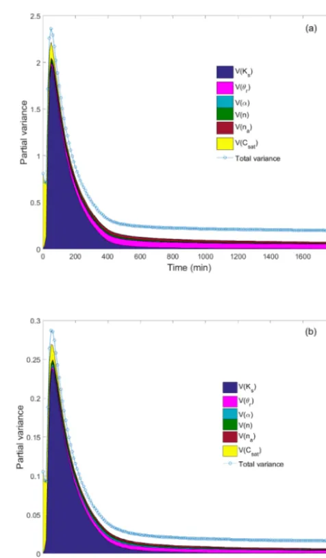
Figure 3.Time distribution of the SP variance at 5 cm(a)and 77 cm (b)depth. The shaded area under the variance curve represents the partial marginal contributions of the random input parameters; the contribution of interactions between parameters is represented by the blank region between the shaded area and the variance curve.

intervals include the reference values reported in Mboh et al. (2012). The sensitivity indices of the six input parame-ters(Ks, θrα, n, na, Csat)are estimated using an experimental design formed byN=212=4096 parameter sets. The order of the sparse PCE is automatically adapted for each observ-able time and location. For some observobserv-able times, the PCE is highly sparse; it reaches a degree of 31 but only contains 112 nonzero coefficients.

Table 1.Reference values, lower and upper bounds for hydraulic and geophysical parameters.

Parameters Lower bounds Upper bounds Reference values

Ks(cm min−1) 0.1 2 0.495

θr(cm3min−3) 0 0.2 0.045

α(cm−1) 0.01 0.2 0.145

n 1.5 7 2.68

na(–) 1 3 1.6

Csat× −10−7(V Pa−1) 2 4 2.9

for sensor 4 (77 cm from the soil surface). Interactions tween parameters are represented by the blank region tween the variance curves and the shaded area. Note that be-cause a Dirichlet boundary condition with zero SP is main-tained at the outlet boundary, the variance of the SP signal is zero at the bottom and reaches its maximum value near the soil surface. Hence, the variance is higher for the first sensor, located 5 cm from the soil surface (Fig. 3a) than for sensor 4, located 77 cm from the soil surface (Fig. 3b).

The SP signals at different altitudes exhibit similar behav-ior (Fig. 3). In the following, we comment on the results of sensor 1 (Fig. 3a). Because Ks varies between 0.1 and 2 cm min−1, the saturated falling-head phase remains until the ponding vanishes attc= −_KLs_sln

Ls Ls+Lw

. Depending on the value ofKs (see Table 1),tcvaries betweent1=20 min andt2=403 min. Thus, in Fig. 3a, we can see that during the first time period(t≤t1), the SP signal is strongly influ-enced by the value of the parameterCsat. The first-order and total sensitivity indices att=10 min (Table 2a) confirm that only the saturated parametersKsandCsatare influential.Csat is about 17 times more influential thanKs. As expected, the remaining parameters have no influence during the first pe-riod. The total variance is 0.72 mv, and there is no interaction between the two parametersKsandCsatsince STi=Si for

both of them andPd

i=1Si=1.

During the second period (t1≤t≤t2), the flow is either saturated or unsaturated depending on the value ofKs. Fig-ure 3a shows that the variance of the SP signal exhibits its maximum value around 2.4 mv, with strong influences of the parameters Ks andCsatand weak interactions between them (small blank region between the variance curve and the shaded area). These results are confirmed by the sensitivity indices calculated att=70 min and reported in Table 2a for sensor 1. Both first-order and total sensitivity indices indi-cate that Ks is the most influential parameter. The second influential parameter isCsat, which has a total sensitivity in-dex about 12 times less thanKs. The parameterαis irrele-vant since its total sensitivity index is 109 times less thanKs and its partial variance is Vi=Si×Vi=0.01 mv, which is

less than the 95 % confidence interval associated with the SP measurement(±0.055 mv). The total variance att=70 min is calculated to be 2.17 mv, and the output–input relationship is close to being additive sincePd

i=1Si=0.94, which means

that interactions between parameters exist but are not signif-icant.

During the third period(t≥t2), the variance of the SP sig-nal reduces to 0.3 mv (Fig. 3a) and significant interactions are observed between parameters (large blank region between the shaded area and the variance curve). Table 2a shows that fort=800 min, which corresponds to dry conditions, the to-tal variance is 0.22. First-order sensitivity indices are very small, except forθr. The latter is highly influential since it has a significant first-order sensitivity index(Si=0.27)and

a more significant total-sensitivity index(STi=0.74). The

parametersCsatandKsare irrelevant as they have very small first-order and total sensitivity indices. Further, strong inter-actions are observed between the parameters since the sum of the first-order indices is far from 1Pd

i=1Si=0.47

. The total sensitivity indices are significantly different from first-order sensitivity indices for almost all parameters. For in-stance, the ratio between these two indices is around 4 forα, 5 fornaand 7 forn. The total sensitivity index ofαremains small (0.065), whereas significant total sensitivity indices are obtained forn (STi=0.27)andna(STi =0.47), which

indi-cates that these two parameters are influential (although their first-order sensitivity indices are small) because of the inter-action between the parameters.

Figure 3b shows similar behavior for sensor 4 located 77 cm from the soil surface. The results in Table 2b indicate that the total variance observed at t=10, 70 and 800 min are around 8 times less than for sensor 1. For the first time period, the first and total sensitivity indices are identical to those observed for sensor 1 since saturated conditions occur inside the whole column and the same effect ofKs andCsat can be observed whatever the location inside the column. For the second time period, the sensitivity indices for sensor 4 (Table 2b) are similar to those observed for sensor 1. How-ever, the results for the third time period show an improve-ment of the relevance of the parameterα, with an increase of both first and total sensitivity indices. Indeed, compared to the results of sensor 1, both first-order and total sensitiv-ity indices tripled. Moreover, the total sensitivsensitiv-ity index for

α (STi =0.22)becomes close to that ofn (STi=0.24).

Table 2.The first-order sensitivity indexSiand the total sensitivity index STi for the SP signal 5(a)and 77 cm(b)below the soil surface at different times.

Ks θr α n na Csat

(cm min−1) (cm3min−3) (cm−1) (V Pa−1)

(a)Sensor 1 (5 cm from the soil surface)

t=10 min (total variance=0.72)

Si 0.055 0 0 0 0 0.942

ST_i 0.057 0 0 0 0 0.945

t=70 min (total variance=2.17)

Si 0.841 0.217 0.005 0.014 0.008 0.045

STi 0.894 0.043 0.008 0.028 0.021 0.078

t=800 min (total variance=0.224)

Si 0.053 0.266 0.015 0.038 0.094 0.008

ST_i 0.085 0.738 0.065 0.266 0.472 0.041

(b)Sensor 4 (77 cm from the soil surface)

t=10 min (total variance=0.094)

Si 0.055 0 0 0 0 0.942

ST_i 0.057 0 0 0 0 0.945

t=70 min (total variance=0.2744)

Si 0.839 0.015 0.014 0.013 0.005 0.053

STi 0.891 0.028 0.024 0.025 0.011 0.086

t=800 min (total variance=0.224)

Si 0.099 0.225 0.054 0.043 0.085 0.01

ST_i 0.138 0.621 0.218 0.238 0.379 0.043

– the parameter Csatis highly influential during the first time period(t≤t1)during which no interactions are ob-served between parameters;

– the parameter Ks is highly influential during the sec-ond time period(t1≤t≤t2)during which small inter-actions occur between parameters;

– the parameters θr, n and na are influential during the third time period (t≥t2)during which dry conditions occur; during this period, strong interactions take place between parameters;

– the parameterαhas no influence on the SP signals dur-ing the two first periods and presents a very small in-fluence (Si=0.015 and STi=0.065)during the third

period on sensor 1 (near the surface of the column); – the relevance of the parameterαimproves with the

dis-tance from the soil surface, although the total variance diminishes with respect to this distance. The influence ofαbecomes significant (STi=0.22)on sensor 4

(lo-cated 77 cm from the soil surface) during the third pe-riod.

4 Parameters’ estimation

4.1 MCMC and FOA approaches

Calibration of computer models is an essential task since some parameters (like the Mualem–van Genuchten-shaped parametersα andn) cannot be directly measured. In such an exercise, the unknown model parameters are investigated by comparing the model responses to the observations. Re-cently, Mboh et al. (2012) showed that the inversion of SP signals can yield an accurate estimate of the saturated hy-draulic conductivityKs, the MVG fitting parametersα and

nand the Archie saturation exponent(na). Moreover, they showed that the quality of the estimation was comparable to that obtained from the calibration of pressure heads. In their study, Mboh et al. (2012) used the FOA approach with the shuffled complex evolution optimization algorithm SCE-UA (Duan et al., 1993).

responses are highly nonlinear functions of model parame-ters (Christensen and Cooley, 1999). In the sequel, the pa-rameter estimation is performed using two approaches: the popular FOA approach and the Bayesian approach based on the MCMC sampler. Contrarily to FOA, the MCMC method is robust since no assumptions of model linearity or differen-tiability are required. Furthermore, prior information avail-able for the parameters can be included. MCMC provides not only an optimal point estimate of the parameters but also a quantification of the entire parameter space. Several MCMC strategies have been developed for Bayesian sampling of the parameter space (Gallagher and Doherty, 2007; Vrugt, 2016). In a groundwater and vadose zone modeling context, the most widely used of these strategies is the Metropolis– Hastings algorithm (Metropolis et al., 1953; Hastings, 1970). It proceeds as follows (Gelman et al., 1996).

i. Choose an initial candidate x0= ξ0, σ0formed by the initial estimate of the parameter setξ0and the hyperpa-rameterσ0 and a proposal distributionq that depends on the previous accepted candidate.

ii. A new candidate xi = ξi, σi is generated from the current one xi−1 with the generator q xixi−1

asso-ciated with the transition probabilityp ξi|ymes, σ

. iii. Calculate p ξi|ymes, σ

and compute the ratio α=

p ξi_|y

mes,σ

qxi xi−1

p(ξi−1_|y

mes,σ)q(xi−1|xi). Additionally, draw a random

numberu∈[0,1] from a uniform distribution.

iv. Ifα≥u, then accept the new candidate, otherwise it is rejected.

v. Resume from (ii) until the chainx0, . . .,xk converges or a prescribed number of iterationsimaxis reached. Many improvements have been proposed in the literature to accelerate the MCMC convergence rate (e.g., Haario et al., 2006; ter Braak and Vrugt, 2008; Dostert et al., 2009, among others). Vrugt et al. (2009a, b) developed the DREAM MCMC sampler based on the differential evolution–Markov chain method of ter Braak (2006) to improve sampling ef-ficiency. DREAM runs multiple Markov chains in paral-lel and uses subspace sampling and outlier chain correction to speed up MCMC convergence (Vrugt, 2016). Laloy and Vrugt (2012) developed the DREAM(ZS)MCMC sampler, in which a candidate for each chain is drawn from an archive of past states denotedZ, which plays the role of the generator

q. Interested readers are referred to Vrugt (2016) for more details about the properties and implementation of DREAM and DREAM(ZS). In the current study, the DREAM(ZS) soft-ware is used for the MCMC estimation of the hydrogeo-physical parameters. Note that because of the large number of model evaluations required, the MCMC method remains rarely used in practical applications compared to the FOA approach. Indeed, with FOA, the CIs are estimated once by

assuming that the Jacobian remains constant within the CIs. This assumption was found to be reasonably accurate in non-linear problems by Donaldson and Scnabel (1987). However, recently, several authors stated that parameter interdepen-dences and model nonlinearities violate this assumption (see, for instance, Vrugt and Bouten, 2002; Vurgin et al. 2007; Gallagher and Doherty, 2007; Mertens et al., 2009; Kahl et al., 2015).

In the following, both MCMC and FOA approaches are employed for the inversion of the highly nonlinear hydro-geophysical problem using SP measurements.

4.2 Parameters estimation results

Hydrogeophysical parameters are estimated using the DREAM(ZS)MCMC sampler (Laloy and Vrugt, 2012). In-dependent uniform distributions are considered for model pa-rameter priors and likelihood hyperpapa-rameters (see Table 1). The parameter posterior distribution is written as

p (ξ|ymes, σ )∝σ−Nexp

−SS(ξ ) 2σ2

, (19)

where SS(ξ )=PN

k=1

ymes(k) −y(k)_mod(ξ ) 2

is the sum of the squared differences between the observedymes(k) and modeled

y_mod(k) SP signals at timetk forN, the total number of SP

ob-servations.

The DREAM(ZS) software computes multiple sub-chains in parallel to thoroughly explore the parameter space. Taking the last 25 % of individuals (when the chains have converged) yields multiple sets used to estimate the updated parameter distributions and therefore the optimal parameter values and their CIs. In the sequel, the DREAM(ZS)MCMC sampler is used with three parallel chains.

We assume that the saturated water content has been ini-tially measured with a fair degree of accuracy. However, instead of fixing its value (as in Kool et al. , 1987, van Dam et al., 1994, and Nützmann et al., 1998, among oth-ers), we assign a Gaussian distribution toθs to take asso-ciated uncertainty and its effect on the estimation of the rest of the parameters into account. It is assumed here that the saturated water content was accurately measured to be

θs=0.43 cm3cm−3by weighing the saturated soil. The cor-responding error measurements are independently and nor-mally distributed with a zero mean and a standard devia-tionσθ =0.01 cm3cm−3. Hence a Gaussian distribution is

hydrogeophysi-Table 3.Estimated mean values (bold), confidence intervals (CIs) and size of the posterior CIs (italic) with MCMC and FOA ap-proaches for scenario 1.

MCMC FOA

Ks 0.49 0.49

(cm min−1) (0.487–0.498) (0.487–0.497)

0.01 0.01

θs 0.43 0.43

(cm3min−3) (0.41–0.45) (0.41–0.45)

0.04 0.04

θr 0.046 0.046

(cm3min−3) (0.025–0.068) (0.026–0.066)

0.04 0.04

α 0.14 0.14

(cm−1) (0.12–0.17) (0.12–0.16)

0.05 0.04

n 2.64 2.64

(2.54–2.77) (2.54–2.76)

0.23 0.22

na 1.64 1.64

(1.37–1.98) (1.38–1.90)

0.6 0.5

Csat 2.90 2.90

(V Pa−1) (2.89–2.91) (2.89–2.91)

0.02 0.02

cal problem investigated, both in the case of abundant data (small uncertainty regions) and in the case of scarcity of data (large uncertainty regions). In the first scenario, SP data col-lected from the sensors located at the five locations are taken into account for the calibration. In the second scenario, only the SP data from the first sensor located 5 cm from the soil surface serve as conditioning information for model calibra-tion. Results of the MCMC sampler are compared to those of the FOA approach for both scenarios.

4.2.1 Scenario 1: inversion using all SP measurements Figure 4 shows the results obtained with MCMC when the SP data of the five sensors are used for the calibration. The “on-diagonal” plots in this figure display the posterior parameter distributions, whereas the “off-diagonal” plots represent the correlations between parameters in the MCMC sample. Fig-ure 4 shows nearly bell-shaped posterior distributions for all parameters. A strong correlation is observed betweenθrand

na(r=0.98).

From the obtained MCMC sample, it is straightforward to estimate the posterior 95 % confidence interval of each rameter. This as well as the mean estimate value of each pa-rameter obtained with both MCMC and FOA approaches are reported in Table 3.

Table 4.Estimated mean values (bold), confidence intervals (CIs) and size of the posterior CIs (italic) with MCMC and FOA ap-proaches for scenario 2.

MCMC FOA

Ks 0.49 0.49

(cm min−1) (0.481–0.495) (0.474–0.503)

0.014 0.029

θs 0.43 0.43

(cm3min−3) (0.41–0.45) (0.41–0.45)

0.04 0.04

θr 0.053 0.053

(cm3min−3) (0.011–0.093) (0.002–0.103)

0.08 0.1

α 0.13 0.13

(cm−1) (0.07–0.20) (-0.15–0.43)

0.13 0.58

n 2.54 2.56

(2.44–2.68) (2.44–2.68)

0.24 0.24

na 1.82 1.78

(1.36–2.41) (1.29–2.27)

1.05 0.98

Csat 2.89 2.89

(V Pa−1) (2.88–2.91) (2.88–2.91)

0.03 0.03

out-Figure 4. MCMC solutions in which all SP data are considered for the calibration. The diagonal plots represent the inferred posterior probability distribution of the model parameters. The off-diagonal scatterplots represent the pairwise correlations in the MCMC drawing.

comes should be interpreted with caution in the context of parameter estimation since (i) a parameter which is not rel-evant for the model output in one sensor can be influential for another sensor and (ii) GSA does not presume the quality of the estimation since two parameters with similar sensitiv-ity indices can have a different qualsensitiv-ity of estimation with the inversion procedure.

Further, the results of Table 3 show that FOA and MCMC approaches yield similar mean estimated values. Moreover, very good agreement is observed between FOA and MCMC uncertainty bounds. Concerning the efficiency of the two cal-ibration methods for this scenario, the FOA approach is by far the most efficient method since it requires only 95 s of CPU time. The MCMC method was terminated after 16 000 model runs, which required 14 116 s. The convergence was reached at around 12 000 model runs. The last 4000 runs were used to estimate the statistical measures of the poste-rior distribution. Recall that contrarily to FOA, MCMC can include prior information available for the parameters and al-lows a quantification of the entire parameter space.

4.2.2 Scenario 2: inversion using only SP measurements near the surface

In this scenario, the number of measurements used for the calibration is strongly reduced. Only SP measurements from sensor 1 (located 5 cm below the soil surface) are considered. The results of MCMC are plotted in Fig. 5. The correlation observed between θr andna decreases slightly tor=0.95. Almost bell-shaped posterior distributions are observed for all parameters except for the parametersθrandα.

The results obtained with MCMC and FOA approaches depicted in Table 4 show the following.

– The FOA approach yields accurate mean estimated val-ues similar to MCMC results for all parameters. – The MCMC and FOA mean estimated values are close

to the reference solution and to the previous scenario. The maximum difference is observed for θr for which the mean estimated value with scenario 2 is 15 % greater than for scenario 1.

– The MCMC CIs for the parametersKs,θs,nandCsatare close to the previous scenario. The parametersθsandn are well estimated (CIs<10 %) and the parametersKs andCsatare very well estimated (CIs≤5 %).

– Due to the reduction of the number of data used for model calibration in scenario 2, the MCMC CIs for the parametersna,αandθrare much larger than in the pre-vious scenario. Indeed, compared to scenario 1, the CI fornaandθrincreases by around 60 %, whereas the CI ofαis 3 times larger than for scenario 1.

– The FOA method yields accurate CIs for the parameters

θs,n,na andCsat, whereas it overestimates the CIs of

θr(by 24 %),Ks(by 100 %) andα(by 427 %). An un-physical uncertainty region (including negative values) is obtained for the parameterα.

These results show that the FOA can fail to provide realis-tic parameter uncertainties and can yield larger CIs than their corresponding nonlinear MCMC counterpart. Indeed, the lin-earization in the FOA method assumes that the Jacobian re-mains constant across the CIs. This assumption was fulfilled for the first scenario in which a large number of measure-ments ensured small uncertainty regions. However, the as-sumption is not fulfilled for some parameters of the current scenario because of the large uncertainty regions induced by the reduction of the number of SP measurements.

Concerning the efficiency of the calibration methods, the FOA required approximately 174 s of CPU time, and the MCMC required many more runs to reach the convergence than in the previous scenario. Indeed, the sampler was used with 50 000 runs (35 000 runs were necessary to reach the convergence).

5 Conclusions

In this work, a synthetic test case dealing with SP signals during a drainage experiment has been studied. The test case is similar to the laboratory experiment developed in Mboh et al. (2012), involving a falling-head infiltration phase fol-lowed by a drainage phase. GSA and Bayesian parameter inference have been applied to investigate (i) the influence of hydraulic and geophysical parameters on the SP signals and (ii) the identifiability of hydrogeophysical parameters us-ing only SP measurements. The GSA was performed usus-ing variance-based sensitivity indices which allow the contribu-tion of each parameter (alone or by interaccontribu-tion with other pa-rameters) to the output variance to be measured. The sensitiv-ity indices have been calculated using a PCE representation of the SP signals. To reduce the number of coefficients and explore PCE with high orders, we used the efficient sparse PCE algorithm developed by Shao et al. (2017), which se-lects the best sparse PCE from a given data set using the Kashyap information criterion (KIC).

The GSA applied to SP signals showed that the parameters

CsatandKsare highly influential during the first period cor-responding to saturated conditions. The parametersθr,nand

naare influential when dry conditions occur. In such condi-tions, strong interactions take place between these parame-ters. The parameterαhas a very small influence on the SP signals near the soil surface but its sensitivity increases with depth although the total variance decreases with depth.

Parameter estimation has been performed using MCMC and FOA approaches to check whether FOA can provide a re-liable estimation of parameters and associated uncertainties for the highly nonlinear hydrogeophysical problem investi-gated. All hydraulic (Ks,θr,αandn)and geophysical (naand

sce-nario for which the whole SP data (measured at five different locations) are used as conditioning information for the model calibration. The confrontation with GSA results shows that the latter should be interpreted with caution when used in the context of parameter estimation since (i) a parameter which is not relevant for the model output in one sensor can be influ-ential for another sensor and (ii) GSA does not presume the quality of the estimation since two parameters with similar sensitivity indices can have a different quality of estimation with the inversion procedure (see, for instance, parametersn

andna). Furthermore, although the studied problem is highly nonlinear, the FOA approach provides accurate estimations of both mean parameter values and CIs in the first scenario. These results are identical to those obtained with MCMC.

When the number of SP measurements used for the cal-ibration is considerably reduced (i.e., data are scarce), the MCMC inversion provides larger uncertainty regions of the parameters. The FOA approach yields accurate mean param-eter values (in agreement with MCMC results) but inaccurate and even unphysical CIs for some parameters with large un-certainty regions.

Data availability. No data sets were used in this article.

Author contributions. AY framed the research question, worked on sensitivity analysis and finalized the manuscript. JZ and FL worked on parameter estimation and numerical model development. MF performed simulations, analyzed the results and reviewed the manuscript.

Competing interests. The authors declare that they have no conflict of interest.

Acknowledgements. The authors acknowledge the financial support from the Tunisian–French joint international laboratory NAILA (http://www.lmi-naila.com/).

Edited by: Bill X. Hu

Reviewed by: two anonymous referees

References

Allègre, V., Jouniaux, L., Lehmann, F., and Sailhac, P.:

Streaming potential dependence on water-content in

Fontainebleau sand, Geophys. J. Int., 182, 1248–1266, https://doi.org/10.1111/j.1365-246X.2010.04716.x, 2010. Archie, G. E.: The Electrical Resistivity Log as an Aid in

Determin-ing Some Reservoir Characteristics, Transactions of the AIME, 146, 54–62, https://doi.org/10.2118/942054-G, 1942.

Arora, B., Mohanty, B. P., and McGuire, J. T.: Uncertainty in dual permeability model parameters for structured soils, Water Re-sour. Res., 48, https://doi.org/10.1029/2011WR010500, 2012.

Belfort, B., Ramasomanan, F., Younes, A., anf Lehmann, F.: An ef-ficient Lumped Mixed Hybrid Finite Element Formulation for variably saturated groundwater flow, Vadoze Zone Journal, 8, 352–362, https://doi.org/10.2136/vzj2008.0108, 2009.

Blatman, G. and Sudret, B.: Efficient computation of global sensitivity indices using sparse polynomial chaos expansions, Reliability Engineering & System Safety, 95, 1216–1229, https://doi.org/10.1016/j.ress.2010.06.015, 2010.

Bogoslovsky, V. A. and Ogilvy, A. A.: Deformation of natural elec-tric fields near drainage structures, Geophys. Prospect., 21, 716– 723. https://doi.org/10.1111/j.1365-2478.1973.tb00053, 1973. Bolève, A., Revil, A., Janod, F., Mattiuzzo, J. L., and Fry, J.-J.:

Preferential fluid flow pathways in embankment dams imaged by self-potential tomography, Near Surf. Geophys., 7, 447–462, https://doi.org/10.3997/1873-0604.2009012, 2009.

Brown, P. N., Hindmarsh, A. C., and Petzold, L. R.: Using Krylov Methods in the Solution of Large-Scale Differential-Algebraic Systems, SIAM J. Sci. Comp., 15, 1467–1488, https://doi.org/10.1137/0915088, 1994.

Carsel, R. F. and Parrish, R. S.: Developing joint probability dis-tributions of soil water retention characteristics, Water Resour. Res., 24, 755–769, https://doi.org/10.1029/WR024i005p00755, 1988.

Christensen, S. and Cooley, R. L.: Evaluation of confidence inter-vals for a steady-state leaky aquifer model, Adv. Water Res., 22, 807–817, https://doi.org/10.1016/S0309-1708(98)00055-4, 1999.

Cukier, R. I., Fortuin, C. M., Shuler, K. E., Petschek, A. G., and Schaibly, J. H.: Study of the sensitivity of coupled reaction sys-tems to uncertainties in rate coefficients, I. theory, J. Chem. Phys., 59, 3873–3878, 1973.

Darnet, M., Marquis, G., and Sailhac, P.: Estimating aquifer hydraulic properties from the inversion of surface Stream-ing Potential (SP) anomalies, Geophys. Res. Lett., 30, https://doi.org/10.1029/2003GL017631, 2003.

Deng, B. and Wang, J.: Saturated-unsaturated groundwater model-ing usmodel-ing 3D Richards equation with a coordinate transform of nonorthogonal grids, Applied Mathematical Modelling, 50, 39– 52, doi10.1016/j.apm.2017.05.021; 2017.

Donaldson, J. R. and Schnabel, R. B.: Computational Ex-perience with Confidence Regions and Confidence In-tervals for Nonlinear Least Squares, Technometrics, 29, https://doi.org/10.2307/1269884, 1987.

Dostert, P., Efendiev, Y., and Mohanty, B.: Efficient uncertainty quantification techniques in inverse problems for Richards’ equa-tion using coarse-scale simulaequa-tion models, Adv. Water Res., 32, 329–339, https://doi.org/10.1016/j.advwatres.2008.11.009, 2009.

Duan, Q. Y., Gupta, V. K., and Sorooshian, S.: Shuffled com-plex evolution approach for effective and efficient global minimization, J. Optimiz. Theory App., 76, 501–521, https://doi.org/10.1007/BF00939380, 1993.

Fahs, M., Younes, A., and Lehmann, F.: An easy and

efficient combination of the Mixed Finite Element

Method and the Method of Lines for the resolution of Richards’ Equation, Environ. Modell. Soft., 24, 1122–1126, https://doi.org/10.1016/j.envsoft.2009.02.010, 2009.

Transport Equations, Water Air. Soil Pollut., 215, 273–283, https://doi.org/10.1007/s11270-010-0477-y, 2011.

Fajraoui, N., Ramasomanana, F., Younes, A., Mara, T. A., Ack-erer, P., and Guadagnini, A.: Use of global sensitivity analysis and polynomial chaos expansion for interpretation of nonreactive transport experiments in laboratory-scale porous media, Water Resour. Res., 47, https://doi.org/10.1029/2010WR009639, 2011. Fajraoui, N., Mara, T. A., Younes, A., and Bouhlila, R.: Reactive Transport Parameter Estimation and Global Sensitivity Analysis Using Sparse Polynomial Chaos Expansion, Water Air. Soil Pol-lut., 223, 4183–4197, https://doi.org/10.1007/s11270-012-1183-8, 2012.

Fajraoui, N., Fahs, M., Younes, A. and Sudret, B.: Analyzing nat-ural convection in porous enclosure with polynomial chaos ex-pansions: Effect of thermal dispersion, anisotropic permeabil-ity and heterogenepermeabil-ity, Int. J. Heat Mass Trans., 115, 205–224, https://doi.org/10.1016/j.ijheatmasstransfer.2017.07.003, 2017. Gallagher, M. and Doherty, J.: Parameter estimation and

uncer-tainty analysis for a watershed model, Environ. Modell. Soft., 22, 1000–1020, https://doi.org/10.1016/j.envsoft.2006.06.007, 2007. Gelman, A., Carlin, J., Stern, H., and Rubin, D.: Bayesian Data Analysis, Second Edition, London, Great Britain: Chapman Hall, 696 p., ISBN:0-158-48838-8, 1996.

Haario, H., Laine, M., Mira, A., and Saksman, E.: DRAM: Efficient adaptive MCMC, Statist. Comput., 16, 339–354, https://doi.org/10.1007/s11222-006-9438-0, 2006.

Hastings, W. K.: Monte Carlo Sampling Methods Using Markov Chains and Their Applications, Biometrika, 57, https://doi.org/10.2307/2334940, 1970.

Hinnell, A. C., Ferré, T. P. A., Vrugt, J. A., Huisman, J. A., Moysey, S., Rings, J., and Kowalsky, M. B.: Improved extrac-tion of hydrologic informaextrac-tion from geophysical data through coupled hydrogeophysical inversion, Water Resour. Res., 46, https://doi.org/10.1029/2008WR007060, 2010.

Ishido, T. and Mizutani, H.: Experimental and theoretical ba-sis of electrokinetic phenomena in rock–water systems and its applications to geophysics, J. Geophys. Res., 86, 1763–1775, https://doi.org/10.1029/JB086iB03p01763, 1981.

Jardani, A., Revil, A., Bolève, A., Crespy, A., Dupont, J.-P., Bar-rash, W., and Malama, B.: Tomography of the Darcy veloc-ity from self-potential measurements, Geophys. Res. Lett., 34, https://doi.org/10.1029/2007GL031907, 2007.

Jougnot, D. and Linde, N.: Self-Potentials in Partially Saturated Me-dia: The Importance of Explicit Modeling of Electrode Effects, Vadose Zone J., 12, https://doi.org/10.2136/vzj2012.0169, 2013. Kahl, G. M., Sidorenko, Y., and Gottesbüren, B.: Local and global inverse modelling strategies to estimate parameters for pesticide leaching from lysimeter studies: Inverse modelling to estimate pesticide leaching parameters from lysimeter studies, Pest Man-age. Sci., 71, 616–631, https://doi.org/10.1002/ps.3914, 2015. Kayshap, R. L.: Optimal choice of AR and MA parts in

autoregres-sive moving average models, IEEE T. Pattern Anal., 4, 99–104, 1982.

Kool, J. B., Parker, J. C., and van Genuchten, M. T.: Parame-ter estimation for unsaturated flow and transport models – A review, J. Hydrol., 91, 255–293, https://doi.org/10.1016/0022-1694(87)90207-1, 1987.

Laloy, E. and Vrugt, J. A.: High-dimensional posterior explo-ration of hydrologic models using multiple-try DREAM (ZS)

and high-performance computing, Water Resour. Res., 48, https://doi.org/10.1029/2011WR010608, 2012.

Linde, N., Jougnot, D., Revil, A., Matthäi, S. K., Arora, T., Renard, D., and Doussan, C.: Streaming current genera-tion in two-phase flow condigenera-tions, Geophys. Res. Lett., 34, https://doi.org/10.1029/2006GL028878, 2007.

Mara, T. A. and Tarantola, S.: Application of global sensitivity anal-ysis of model output to building thermal simulations, Build. Sim., 1, 290–302, https://doi.org/10.1007/s12273-008-8129-5, 2008. Mara, T. A., Belfort, B., Fontaine, V., and Younes, A.:

Ad-dressing factors fixing setting from given data: A compari-son of different methods, Environ. Modell. Soft., 87, 29–38, https://doi.org/10.1016/j.envsoft.2016.10.004, 2017.

Mboh, C. M., Huisman, J. A., Zimmermann, E., and Vereecken, H.: Coupled Hydrogeophysical Inversion of Streaming Potential Signals for Unsaturated Soil Hydraulic Properties, Vadose Zone J., 11, https://doi.org/10.2136/vzj2011.0115, 2012.

Mertens, J., Kahl, G., Gottesbüren, B. and Vanderborght, J.: Inverse Modeling of Pesticide Leaching in Lysimeters: Local versus Global and Sequential Single-Objective ver-sus Multiobjective Approaches, Vadose Zone J., 8, 793, https://doi.org/10.2136/vzj2008.0029, 2009.

Metropolis, N., Rosenbluth, A. W., Rosenbluth, M. N., Teller, A. H., and Teller, E.: Equation of State Calculations by Fast Computing Machines, J. Chem. Phys., 21, 1087–1092, https://doi.org/10.1063/1.1699114, 1953.

Miller, C. T., Williams, G. A., Kelley, C. T., and Tocci, M. D.: Robust solution of Richards’ equation for nonuni-form porous media, Water Resour. Res., 34, 2599–2610, https://doi.org/10.1029/98WR01673, 1998.

Mualem, Y.: A new model for predicting the hydraulic conductivity of unsaturated porous media, Water Resour. Res., 12, 513–522, https://doi.org/10.1029/WR012i003p00513, 1976.

Nützmann, G., Thiele, M., Maciejewski, S., and Joswig, K.: In-verse modelling techniques for determining hydraulic properties of coarse-textured porous media by transient outflow methods, Adv. Water Res., 22, 273–284, https://doi.org/10.1016/S0309-1708(98)00009-8, 1998.

Patella, D.: Introduction to ground surface self-potential

tomography, Geophys. Prospect, 45, 653–681,

https://doi.org/10.1046/j.1365-2478.1997.430277, 1997. Rajabi, M. M., Ataie-Ashtiani, B., and Simmons, C. T.:

Polynomial chaos expansions for uncertainty propaga-tion and moment independent sensitivity analysis of sea-water intrusion simulations, J. Hydrol., 520, 101–122, https://doi.org/10.1016/j.jhydrol.2014.11.020, 2015.

Revil, A., Linde, N., Cerepi, A., Jougnot, D., Matthäi, S., and Finsterle, S.: Electrokinetic coupling in unsaturated porous media, J. Colloid Interface Sci., 313, 315–327, https://doi.org/10.1016/j.jcis.2007.03.037, 2007.

Richards, K., Revil, A., Jardani, A., Henderson, F., Batzle, M., and Haas, A.: Pattern of shallow ground water flow at Mount Princeton Hot Springs, Colorado, using geoelec-tric methods, J. Volcanol. Geotherm. Res., 198, 217–232, https://doi.org/10.1016/j.jvolgeores.2010.09.001, 2010. Riva, M., Guadagnini, A., and Dell’Oca, A.:

Sailhac, P. and Marquis, G.: Analytic potentials for the for-ward and inverse modeling of SP anomalies caused by subsurface fluid flow, Geophy. Res. Lett., 28, 1851–1854, https://doi.org/10.1029/2000GL012457, 2001.

Saltelli, A., Tarantola, S., and Chan, K. P.-S.: A Quantita-tive Model-Independent Method for Global Sensitivity Analysis of Model Output, Technometrics, 41, 39–56, https://doi.org/10.1080/00401706.1999.10485594, 1999. Shao, Q., Younes, A., Fahs, M., and Mara, T. A.: Bayesian

sparse polynomial chaos expansion for global sensitiv-ity analysis, Comput. Method Appl. M., 318, 474–496, https://doi.org/10.1016/j.cma.2017.01.033, 2017.

Sobol’, I. M.: Global sensitivity indices for nonlinear mathematical models and their Monte Carlo estimates, Math. Comput. Sim., 55, 271–280, https://doi.org/10.1016/S0378-4754(00)00270-6, 2001.

Sobol’, I. M.: Sensitivity estimates for nonlinear mathematical mod-els, Math. Model. Comput. Exp., 407–414, 1993.

Sudret, B.: Global sensitivity analysis using polynomial chaos expansions, Reliab. Eng. Syst. Safe., 93, 964–979, https://doi.org/10.1016/j.ress.2007.04.002, 2008.

ter Braak, C. J. F.: A Markov Chain Monte Carlo version of the genetic algorithm differential evolution: Easy Bayesian com-puting for real parameter spaces, Stat Comput., 16, 239–249, https://doi.org/10.1007/s11222-006-8769-1, 2006.

ter Braak, C. J. F. and Vrugt, J. A.: Differential Evolution Markov Chain with snooker updater and fewer chains, Statist. Comput., 18, 435–446, https://doi.org/10.1007/s11222-008-9104-9, 2008. van Dam, J. C., Stricker, J. N. M., and Droogers, P.: In-verse Method to Determine Soil Hydraulic Functions from Multistep Outflow Experiments, Soil Sci. Soc. Am. J., 58, https://doi.org/10.2136/sssaj1994.03615995005800030002x, 1994.

van Genuchten, M. T.: A Closed-form Equation

for Predicting the Hydraulic Conductivity of

Un-saturated Soils, Soil Sci. Soc. Am. J., 44, 892,

https://doi.org/10.2136/sssaj1980.03615995004400050002x, 1980.

Volkova, E., Iooss, B., and Van Dorpe, F.: Global sensitivity analysis for a numerical model of radionuclide migration from the RRC “Kurchatov Institute” radwaste disposal site, Stoch. Env. Res. Risk A., 22, 17–31, https://doi.org/10.1007/s00477-006-0093-y, 2008.

Vrugt, J. A., Gupta, H. V., Bouten, W. and Sorooshian, S.: A Shuf-fled Complex Evolution Metropolis algorithm for optimization and uncertainty assessment of hydrologic model parameters, Wa-ter Resour. Res., 39, doi:10.1029/2002WR001642, 2003. Vrugt, J. A. and Bouten, W.: Validity of First-Order Approximations

to Describe Parameter Uncertainty in Soil Hydrologic Models, Soil Sci. Soc. Am. J., 66, https://doi.org/10.2136/sssaj2002.1740, 2002.

Vrugt, J. A., ter Braak, C. J. F., Clark, M. P., Hyman, J. M., and Robinson, B. A.: Treatment of input uncertainty in hydrologic modeling: Doing hydrology backward with Markov chain Monte Carlo simulation: FORCING DATA ER-ROR USING MCMC SAMPLING, Water Resour. Res., 44, https://doi.org/10.1029/2007WR006720, 2008.

Vrugt, J. A., ter Braak, C. J. F., Diks, C. G. H., Robin-son, B. A., Hyman, J. M., and Higdon, D.: Accelerat-ing Markov chain Monte Carlo simulation by differen-tial evolution with self-adaptive randomized subspace sam-pling, Int. J. Nonlinear Sci. Numer. Simul., 10, 273–290, https://doi.org/10.1515/IJNSNS.2009.10.3.273, 2009a.

Vrugt, J. A.: Markov chain Monte Carlo simulation using the DREAM software package: Theory, concepts, and MAT-LAB implementation, Environ. Modell. Soft., 75, 273–316, https://doi.org/10.1016/j.envsoft.2015.08.013, 2016.

Vrugt, J. A., Robinson, B. A., and Hyman, J. M.: Self-adaptive multimethod search for global optimization in real parameter spaces, IEEE Trans. Evol. Comput., 13, 243–259, https://doi.org/10.1109/TEVC.2008.924428, 2009b.

Vugrin, K. W., Swiler, L. P., Roberts, R. M., Stucky-Mack, N. J., and Sullivan, S. P.: Confidence region estima-tion techniques for nonlinear regression in groundwater flow: Three case studies, Water Resour. Res., 43, W03423, https://doi.org/10.1029/2005WR004804, 2007.

Wiener, N.: The Homogeneous Chaos, Am. J. Math., 60, https://doi.org/10.2307/2371268, 1938.

Younes, A., Fahs, M., and Ahmed, S.: Solving density driven flow problems with efficient spatial discretizations and higher-order time integration methods, Adv. Water Res., 32, 340–352, https://doi.org/10.1016/j.advwatres.2008.11.003, 2009. Younes, A., Fahs, M., and Belfort, B.: Monotonicity of the

cell-centred triangular MPFA method for saturated and unsaturated flow in heterogeneous porous media, J. Hydrol., 504, 132–141, https://doi.org/10.1016/j.jhydrol.2013.09.041, 2013.

Younes, A., Mara, T. A., Fajraoui, N., Lehmann, F., Belfort, B., and Beydoun, H.: Use of Global Sensitivity Analysis to Help As-sess Unsaturated Soil Hydraulic Parameters, Vadose Zone J., 12, https://doi.org/10.2136/vzj2011.0150, 2013.

Younes, A., Delay, F., Fajraoui, N., Fahs, M., and Mara, T. A.: Global sensitivity analysis and Bayesian param-eter inference for solute transport in porous media

col-onized by biofilms, J. Contam. Hydrol., 191, 1–18,

https://doi.org/10.1016/j.jconhyd.2016.04.007, 2016.

Younes, A., Mara, T., Fahs, M., Grunberger, O., and Ackerer, P.: Hydraulic and transport parameter assessment using column in-filtration experiments, Hydrol. Earth Syst. Sci., 21, 2263–2275, https://doi.org/10.5194/hess-21-2263-2017, 2017.