https://doi.org/10.5194/hess-23-2897-2019 © Author(s) 2019. This work is distributed under the Creative Commons Attribution 4.0 License.
On the uncertainty of initial condition and initialization
approaches in variably saturated flow modeling
Danyang Yu1, Jinzhong Yang1, Liangsheng Shi1, Qiuru Zhang1, Kai Huang2, Yuanhao Fang3, and Yuanyuan Zha1 1State Key Laboratory of Water Resources and Hydropower Engineering Sciences,
Wuhan University, Wuhan, Hubei 430072, China
2Guangxi Hydraulic Research Institute, Nanning, Guangxi 530023, China
3School of Earth Sciences and Engineering, Hohai University, Nanjing, Jiangsu 210098, China Correspondence:Yuanyuan Zha ([email protected])
Received: 4 November 2018 – Discussion started: 20 December 2018 Revised: 28 April 2019 – Accepted: 13 June 2019 – Published: 12 July 2019
Abstract. Soil water movement has direct effects on envi-ronment, agriculture and hydrology. Simulation of soil water movement requires accurate determination of model parame-ters as well as initial and boundary conditions. However, it is difficult to obtain the accurate initial soil moisture or matric potential profile at the beginning of simulation time, mak-ing it necessary to run the simulation model from the arbi-trary initial condition until the uncertainty of the initial con-dition (UIC) diminishes, which is often known as “warming up”. In this paper, we compare two commonly used methods for quantifying the UIC (one is based on running a single simulation recursively across multiple hydrological years, and the other is based on Monte Carlo simulations with real-ization of various initial conditions) and identify the warm-up timetwu(minimum time required to eliminate the UIC by warming up the model) required with different soil textures, meteorological conditions and soil profile lengths. Then we analyze the effects of different initial conditions on parame-ter estimation within two data assimilation frameworks (i.e., ensemble Kalman filter and iterative ensemble smoother) and assess several existing model initializing methods that use available data to retrieve the initial soil moisture profile. Our results reveal that Monte Carlo simulations and the recursive simulation over many years can both demonstrate the tempo-ral behavior of the UIC, and a common threshold is recom-mended to determinetwu. Moreover, the relationship between
twufor variably saturated flow modeling and the model set-tings (soil textures, meteorological conditions and soil profile length) is quantitatively identified. In addition, we propose a
warm-up period before assimilating data in order to obtain a better performance for parameter and state estimation.
1 Introduction
Many publications have addressed the issue of the uncer-tainty of the initial condition (UIC) in modeling soil water movement. For example, Walker and Houser (2001) com-pared the simulation with the degraded soil moisture initial condition to that with the true initial condition and found that the discrepancy did not fade away even after 1 month. Then, Mumen (2006) concluded that the initial soil water state was one of the most important factors for estimating soil moisture in the case of bare soil. Chanzy et al. (2008) tested three ini-tial water potenini-tial profiles and found that iniini-tialization had a strong impact on the soil moisture prediction. These stud-ies showed that the incorrect initial condition may lead to false results. Based on the availability of information, differ-ent initialization approaches can be used for constructing ini-tial conditions, e.g., an arbitrary uniform profile (Chanzy et al., 2008; Das and Mohanty, 2006; Varado et al., 2006), a lin-ear interpolation with in situ observation (Bauser et al., 2016) or a steady-state soil moisture profile induced with a constant infiltration flux (Freeze, 1969). All of the approaches involve great uncertainties due to nonlinearity of soil moisture pro-file, observation error or the inaccurate boundary condition. As a result, it is crucial to explore the effects of the UIC on model outputs and compare the uncertainties inherited from various initialization approaches.
Besides the simple initialization methods referred to above, another common approach is to obtain the initial condition inherited from the warm-up model with preced-ing meteorological data. Startpreced-ing from an arbitrary initial condition, this approach runs the model using a certain pe-riod (i.e., warm-up time twu) of meteorological data until the model state (e.g., soil moisture) reaches an equilibrium state, which is defined as the state when the uncertainty orig-inating from the UIC is negligible during simulation. The equilibrium state can be obtained by either running Monte Carlo simulations until the states from different initial con-ditions converge to the same value (hereafter referred to as the Monte Carlo method; Chanzy et al., 2008) or running a single simulation for several years by repeating a 1-year or multiple-year meteorological condition until the state at an arbitrary date ceases to vary from year to year (spin-up method; DeChant and Moradkhani, 2011; Seck et al., 2014). The spin-up method is widely used in large-scale hydrolog-ical model due to its smaller computational cost, while the less-common Monte Carlo method has the merit of quanti-fying the UIC explicitly at arbitrary time, which can be po-tentially used to construct state covariance matrix for data assimilation. To the best of our knowledge, there is no com-parison made between these two methods to date. Finding an equivalency between these two methods is beneficial for link-ing initialization methods and data assimilation techniques. Moreover, the determination of warm-up timetwuis crucial to the success of this approach (Ajami et al., 2014; Rahman and Lu, 2015). An underestimation oftwumay bring uncer-tainty from an arbitrarily specified initial condition prior to initialization, while a largetwuleads to higher computational
demands (Rodell et al., 2005). A variety of modeling settings, such as soil hydraulic properties, meteorological conditions and soil profile lengths, have strong influences ontwu(Ajami et al., 2014; Cosgrove et al., 2003; Lim et al., 2012; Walker and Houser, 2001). Thus, the determination oftwushould be investigated thoroughly with different settings.
As well as model predictions, the UIC also has consid-erable effects on parameter estimation. One of the com-monly used inverse methods in the field of vadose zone hy-drology is the data assimilation approach (Vereecken et al., 2010; Chirico et al., 2014; Medina et al., 2014a, b). Pre-vious studies showed that a poor initial soil moisture pro-file can be corrected by assimilating near-surface measure-ments (Galantowicz et al., 1999; Walker and Houser, 2001; Das and Mohanty, 2006). Oliver and Chen (2009) discussed several possible approaches for improving the performance of data assimilation through improved sampling of the ini-tial ensemble and suggested the use of the pseudo-data. Re-cently, Tran et al. (2013) found that decreasing assimilation interval could improve the soil moisture profile results in-duced by the wrong initial condition, and Bauser et al. (2016) addressed the importance of the UIC in the data assimila-tion framework. However, these preliminary investigaassimila-tions of the influence of the UIC in data assimilation results are de-graded by the narrow choice of initialization and data assim-ilation methods and the lack of comprehensive assessment of the temporal evolution of state or parameter uncertainty when the UIC and the parameter uncertainty coexist. For in-stance, during data assimilation, the initial ensemble is often assumed to be known without uncertainty (Shi et al., 2015) or created by adding Gaussian noise to the initial estimate (Huang et al., 2008), both of which may result in false out-puts. The researches mentioned above are all based on a se-quential data assimilation approach (i.e., ensemble Kalman filter or EnKF; Walker and Houser, 2001; Oliver and Chen, 2009), which incorporates observation in a sequential fashion so that the effect of the UIC can be eliminated quickly. Com-pared to EnKF, an iterative ensemble smoother (IES), which assimilates all data available simultaneously, can obtain rea-sonably good history-matching results and performs better in strongly nonlinear problems (Chen and Oliver, 2013). How-ever, the IES utilizes all the observation simultaneously at every iteration, and the UIC may have a more persistent ef-fect on the IES. Thus, a systematical analysis for the efef-fects of the UIC and initialization methods within various data as-similation frameworks is necessary and obligatory.
different data assimilation frameworks to minimize the influ-ence of the UIC. We first summarize the governing equations of variably saturated flow and methods of the UIC quantifi-cation in Sect. 2. Then we present results of synthetic sim-ulations designed to investigate the propagation of the UIC under different scenarios in Sect. 3, which is complemented by the results for field data in Sect. 4. Finally, we present our conclusions in Sect. 5.
2 Method
2.1 One-dimensional soil water movement
Richards’ equation can be used to describe the one-dimensional, vertical soil water movement, which is given as ∂θ ∂t = ∂ ∂z K ∂h
∂z+1
, (1)
whereh(L) represents the pressure head,θ(–) denotes volu-metric soil moisture,t(T) indicates the time,z(L) is the spa-tial coordinate taken positive upward andK(L T−1) denotes the unsaturated hydraulic conductivity. The solution of the one-dimensional Richards’ equation is numerically solved by a noniterative numerical scheme, which was originally pro-posed in Ross (2003). By using the primary variable switch-ing scheme, this scheme uses the soil moisture as the un-known variable for unsaturated nodes and the pressure head for saturated nodes (Zha et al., 2013). It can greatly reduce the computational cost of variably saturated flow modeling in soils under the atmospheric boundary condition, where al-ternative drying–wetting conditions are often encountered.
To obtain the solution of Eq. (1), the knowledge of func-tionsKandθversushmust be required. In this study, we use the van Genuchten–Mualem model (van Genuchten, 1980; Mualem, 1976) to describe these relationships:
θ (h)=θr+
θs−θr
[1+ |αh|n]m, (2)
K(θ )=KsSe0.5
h
1−1−Se1/m
mi2
, (3)
whereKs(L T−1) denotes the saturated hydraulic conductiv-ity,θs andθrrepresent the saturated and residual soil mois-ture, respectively, parametersα(L−1) andnare related to the measure of the pore-size density functions andm=1−1/n
(n >1), and the effective saturation degreeSe is defined as
Se=(θ−θr)/(θs−θr).
Initial and boundary conditions are needed to solve the one-dimensional Richards’ equation. The initial condition could be the state of soil moisture,
θ (z, t )|t=0=θ0(z) , (4)
whereθ0(z)is the initial soil moisture profile.
The state-dependent, atmospheric boundary condition can be described as (Šim˚unek et al., 2013)
|q| =
−K∂h ∂z−K
≤Ep−Pp
, (5)
hm> h > hc, (6)
where q (L T−1) is the Darcian flux at the soil surface,
Ep (L T−1) denotes the potential evaporation, Pp (L T−1) represents the precipitation intensity, andhm(L) andhc(L) are maximum and minimum pressure heads allowed at the soil surface, respectively. The value ofhmis set to 0, whereas
hcis determined as−100 m.
The bottom boundary condition is the free drainage bound-ary:
∂h ∂z
z=zN =0, (7)
wherezNis the depth of bottom boundary. 2.2 UIC quantification
The investigation of uncertainty in this study includes model states (e.g., soil moisture) and model parameters, where the UIC is a special case of state uncertainty att=0. The analy-sis is twofold. First, we consider a particular situation when the UIC is the only uncertain source and all the model pa-rameters are known. Thus, the choice of initial conditions is solely responsible for the accuracy of the model outputs. In this case, the temporal decay of the UIC can be clearly demonstrated by utilizing the spin-up or Monte Carlo meth-ods. Second, a more complex and realistic situation, includ-ing both the uncertain initial condition and model parame-ters, is considered during the data assimilation of soil mois-ture observation. The UIC and data assimilation are smoothly combined in our approach, since we choose Monte Carlo-based methods (EnKF and IES). At t=0, we generate an ensemble of soil moisture profiles based on one initializa-tion method (which introduces UIC) and use this ensemble to initiate the data assimilation (assimilate observations and estimate parameter). Finally, we can evaluate our data assim-ilation performance based on different initializing methods. 2.2.1 The indices of spin-up and Monte Carlo methods The uncertainty of the initial condition can be measured by the percent change (PC) for the spin-up method (Ajami et al., 2014; Seck et al., 2014) or the ensemble spreadSp for the Monte Carlo method (Reichle and Koster, 2003). Percent change is an index that reflects the deviation of soil moisture between 2 adjacent years in a recursive run after a period of warm-up timetwu, which could be calculated as
PC(t )=100
M(t )−M(t+12) M(t+12)
where M(t ) and M(t+12) are the monthly averaged soil moisture after model spin-up fortmonths andt+12 months (De Goncalves et al., 2006).
The ensemble spread (Sp), calculated as a square root of averaged variance over all interested nodes, is an index for quantifying the difference among various realizations in the Monte Carlo simulation, and it is given as
Sp(k)=
v u u t
1
N (Ne−1) N X
i=1 Ne
X
j=1
yi,j,ka −yi,ka
2
, (9)
whereyi,j,ka is nodal soil moisture value,hyi,ka iis the ensem-ble mean of yi,j,ka , i=1, 2, . . . ,N values are the nodes of interest (can be part of the profile), j=1, 2, . . . ,Ne is the ensemble number index andNeis the ensemble size, which is taken as 300 in this study, based on sensitivity analysis of the ensemble size on the calculated results. WhenN=1, the concept ofSp(k)is equivalent to the standard deviation ofyka at one location and timetk.
2.2.2 Data assimilation approaches
We employ EnKF and the IES for data assimilation in this study. Figure 1 illustrates the basic ideas and differences of the two methods.
The EnKF approach was first proposed by Evensen (1994) and has been widely used in variably saturated flow problems (Huang et al., 2008; De Lannoy et al., 2007). This approach is a sequential data assimilation method (as shown in Fig. 1a) which incorporates observations into the model in order.
In this part, we assume that hydraulic parameters Ks, α
andnare unknown, while the other parametersθrandθs are deterministic. The vector of the parameter and state is de-scribed as
yk=[mk,uk]T, (10) wheremk is the parameter vector (i.e.,Ks,αandn),uk is state variables (i.e., soil moisture) at time tk, the dimension ofyk isNy:Ny=Nm+Nd, whereNmindicates the amount of the parameters to be estimated, and Ndis the number of nodes of the numerical model. The updated soil moisture en-semble can be converted to the pressure head to drive the model. The observation vector can be defined as
dj,k=dk+εj,k, (11) wheredkdenotes the observations at timetk,εj,kvalues (j= 1, 2, . . . ,Ne) are independent Gaussian noises added to the observations anddj,kis the observation vector for ensemble indexjat timetk. Based on the differences of model forecast and observations, the state–parameter vector can be updated to
yaj,k=yfj,k+Kk
dj,k−Hyfj,k
, (12)
whereyfj,k denotes the estimated or initially guessed values of parameter and state, whileyaj,k is the updated estimates, andHis an observation operator, linking the relationship be-tween the state–parameter vector and the observation vector. Krepresents the Kalman gain matrix, which can be calcu-lated as
KK=CfkHT h
HCfkHT+CDK
i−1
, (13)
whereCDk indicates the covariance matrix of observed data
errors, whileCfk is the error covariance matrix of forecast ensemble, given by
Cfk≈ 1 Ne−1
Ne
X
j=1
h
yfj,k−DyfkEi hyfj,k−DyfkEiT
, (14)
wherehyf
kiis the ensemble mean ofyfk.
Compared to EnKF, the IES gives a better estimate by taking all the available observations into consideration (van Leeuwen and Evensen, 1996), as presented in Fig. 1b. Thus, it can keep the overall consistency of parameters and state variables over time effectively and has been increas-ingly used to solve the parameter estimation problem in hy-drology (Crestani et al., 2013; Emerick and Reynolds, 2013). By calculating iteratively, the nonlinear relationship between observation and parameter is linearized and the information content of the observations can be fully utilized (Chen and Oliver, 2013). In this case, we write the analyzed vector of model parametersmrj as
mrj+1=mrj+Krdrj−Hmrj. (15) The notation is similar to the one presented for EnKF, where “r” is the iteration index,mrj is the initially guessed or esti-mated parameters for realizationj at iterationr, andmrj+1is the updated estimates for realizationjby conditioning on the observed information at iterationr. It should be noted that thedrj andHmr
jdenote the total number of observations and predicted data at iterationr, which is different from EnKF. The Kalman gainKis defined as
Kr=CfrHThHCfrHT+CD+λdiag
HCfrHTi
−1
, (16)
Figure 1.Flow charts of simulation period – or data assimilation period with(a)ensemble Kalman filter (EnKF) and(b)iterative ensemble smoother (IES) – and warm-up period.t0is the initial time, andtend is the end of simulation time.mk anduk are the vectors of model parameters (e.g., hydraulic conductivity) and state variables (e.g., soil moisture), respectively, at timetk, whilemrandurare the vectors at iterationr; the superscripts “a” and “f” refer to model analysis and forecast (or initial guess). Besides this, the period betweentpreandt0
donates the process of warming up, andtwuis the required warm-up time.
2.2.3 Quantitative index for data assimilation
To assess model parameter and state estimations, the root-mean-square error (RMSE) of estimated parame-ters (RMSEm) and soil moisture (RMSEobs) and the relative error index (RE) are computed as follows:
RMSEm=
v u u t
1
Ne Ne
X
j=1
mEj−mT2, (17)
RMSEobs= v u u t
1
Nobs Nobs
X
n=1
dne−dnobs 2
, (18)
RE=RMSE e m RMSEpm
, (19)
wheremEj represents the estimated parameter of realizationj
at the last simulation day (EnKF) or the last iteration (IES) andmTrepresents the true parameter listed in Table 1.dneand
dnobs indicate the predicted and measured soil moisture, re-spectively.Nobsis the amount of observations. RMSEemand RMSEpmrepresent the RMSE of the estimated and prior pa-rameters, respectively. RE varies from 0 to positive infinity. As RE approaches 0, the analysis result is close to the truth, but a large value of RE (more than 1) indicates a bad pa-rameter estimation. Compared with the RMSEm, this index can better present the improvement of parameter estimation during data assimilation.
3 Numerical examples
[image:5.612.310.545.345.412.2]A series of synthetic numerical experiments are performed in this section. In Sect. 3.1, we give a general description
Table 1.Soil hydraulic parameters used in simulation.
Soil θs θr Ks(m d−1) α(m−1) n
Sand 0.43 0.045 7.128 14.5 2.68 Loam 0.43 0.078 0.2496 3.6 1.56 Silt 0.46 0.034 0.06 1.6 1.37 Clay loam 0.41 0.095 0.062 1.9 1.31
of the numerical experiments. In order to gain a better un-derstanding of the propagation of the UIC, all the hydraulic parameters (i.e.,Ks,αandn) are deterministic, and the UIC is the only uncertainty source in Sect. 3.2. Finally, the nu-merical cases are designed to evaluate performances of data assimilation algorithms combined with various initialization methods in Sect. 3.3, in which the parameter uncertainty is taken into consideration in conjunction with the UIC. 3.1 General description of model inputs
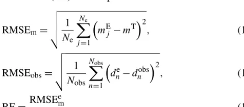
As shown in Table 1, four soils (sand, loam, silt and clay loam) are chosen in this study to explore the impacts of soil hydraulic property on the UIC. The values of hydraulic parameters are determined according to Carsel and Par-rish (1988). Besides this, the effects of the meteorological condition are also considered: M-AC, M-SC and M-HC in Fig. 2 represent three sets of precipitation and potential evap-oration data from three different regions (arid region, semi-arid region and humid region) in China.
[image:5.612.46.285.401.506.2]Figure 2.Synthetic rainfall (blue bars) and potential evaporation (red bars) of three typical climates:(a)arid climate,(b)semi-arid climate and(c)humid climate. It should be noted that the meteorological data of simulation period are from day 366 to day 730.
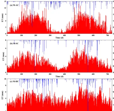
is discretized into 60 grids with a grid size of 5 cm, which has been proved to be sufficient for evaluating the UIC in our study (results not shown). Besides this, the total simula-tion time during the synthetic simulasimula-tion is 1 year (365 d). In addition, the default upper and bottom boundaries are set to be M-SC and the free drainage boundary, respectively. Other specifications and assumptions for our model simulation runs are given in Table 2.
3.2 The temporal evolution of UIC
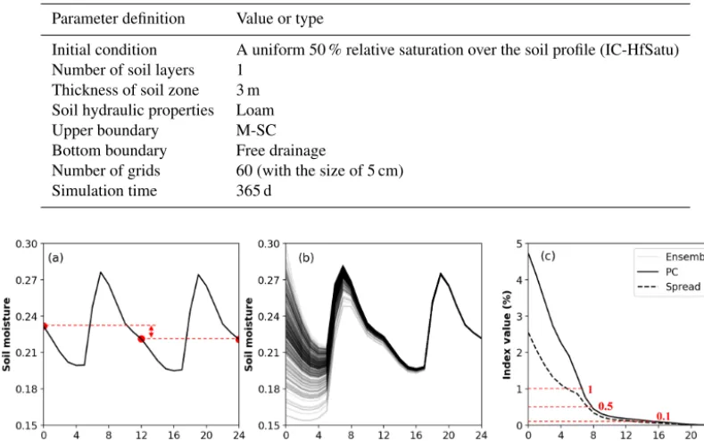
3.2.1 Comparison of UIC quantification methods A synthetic experiment is conducted to compare two meth-ods (i.e., spin-up method and Monte Carlo method) in quanti-fying the UIC. Using the spin-up method, the first case runs a single simulation for 10 years by repeating the preceding
me-teorological condition starting with IC-HfSatu (Fig. 3a), and the percentage cutoff PC is calculated. In the second case, the Gaussian noise with a standard deviation of 3 % (deter-mined according to the observation error of soil moisture) is added to the IC-HfSatu to generate an ensemble with differ-ent initial soil moisture profiles. Then we run differdiffer-ent model realizations (Fig. 3b). Finally, the PC andSpvalues of the two cases versus time are compared in Fig. 3c.
Table 2.The default model settings used in the simulations.
Parameter definition Value or type
Initial condition A uniform 50 % relative saturation over the soil profile (IC-HfSatu) Number of soil layers 1
Thickness of soil zone 3 m Soil hydraulic properties Loam Upper boundary M-SC Bottom boundary Free drainage
Number of grids 60 (with the size of 5 cm) Simulation time 365 d
Figure 3.Comparison of spin-up and Monte Carlo methods in determining warm-up time.(a)The spin-up method with monthly averaged soil moisture versus time by running a simulation recursively for 10 years,(b)Monte Carlo method with monthly averaged soil moisture of different realizations versus time based on various initial conditions, and(c)comparison of PC andSpversus time. For the purpose of
demonstration, the parameter uncertainty is not considered, and we only show the results of the first 2 years in the figure.
4.7 % and Spof 2.6 %) is due to different initial soil mois-ture values given by the spin-up and Monte Carlo methods. The result indicates that the widely used the spin-up method and Monte Carlo method are equivalent in terms of quanti-fying the UIC. We will use Monte Carlo method for the rest of the study, since it is consistent with the data assimilation approaches used in this study.
The determination of the threshold value when the UIC is regarded to have negligible effects on modeling has been discussed in previous studies (Ajami et al., 2014; Lim et al., 2012; Seck et al., 2014). PC orSp values of 1 % (Yang et al., 1995), 0.1 % (De Goncalves et al., 2006) or 0.01 % (Henderson-Sellers et al., 1993) have been used. As shown in Fig. 3c, there is a significant diversity in the results between the spin-up and Monte Carlo methods at the index value of 1 %, indicating that the UIC still plays a significant role. In contrast, the requestedtwuis more than 15 months for a value of 0.1 %. To balance the estimation accuracy and computa-tional cost, we recommend a threshold of 0.5 % for both the spin-up and Monte Carlo methods; the corresponding warm-up timetwuis 8 months, which is long enough for the UIC to diminish, and the difference between PC andSpis insignifi-cant.
3.2.2 The influencing factors on UIC
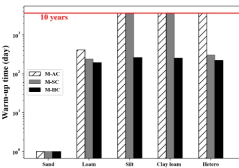
The Monte Carlo method is used in this part to obtain the warm-up timetwu, and a number of scenarios are constructed under a variety of conditions (different soils, meteorological conditions and soil profile lengths). First, the influence of soil texture and the meteorological condition on twu are exam-ined. Four different types of homogeneous soils (sand, loam, silt and clay loam listed in Table 1) and a heterogeneous soil with multiple layers – consisting of loam (0–75 cm), clay loam (75–150 cm), silt (150–225 cm) and sand (225–300 cm) – under three typical meteorological conditions (AC, M-SC and M-HC) are employed in these scenarios, while the other model inputs use the default values (see Table 2). Be-sides this, the influence of different soil profile lengths (1, 3, 5, 10, 15 and 20 m) on the UIC is also investigated.
a. The influences of soil texture and meteorological condition
Figure 4.The length of warm-up timetwuwith various soils and
meteorological conditions. Note that some of the twu values are
larger than 10 years and are not able to be obtained due to the 10-year simulation time. The heterogeneous soil profile consists of loam (0–75 cm), clay loam (75–150 cm), silt (150–225 cm) and sand (225–300 cm).
with M-HC are 264 and 253 d. The results imply that the warm-up timetwufor the fine-textured soil is larger than that for coarse-textured soil. This may be attributed to the diver-sity of the drainage property for different soils. For sand, due to its fast drainage property, the soil moisture ensemble con-verges extremely quickly and most of the values at the profile are maintained as residual soil moisture. Thus, the UIC of sand disappears very quickly. In contrast, the soil moisture states for silt and clay loam change more slowly than sand during the simulation. Therefore, the faster drainage prop-erty leads to a smaller warm-up time.
In addition, the meteorological condition has a strong im-pact on the UIC. For example, with soil loam, the order oftwu is M-HC<M-SC<M-AC. For silt and clay loam,twu val-ues of M-AC and M-SC decrease from more than 10 years to 264 and 253 d with a humid climate M-HC, respectively. With intensive and excessive rainfall events, θ approaches the saturated soil moisture, leading to a sudden drop in Sp. Thus, the meteorological condition, especially the precipita-tion, plays an important role in the propagation of the UIC. Moreover, regarding the heterogeneous soil with multiple layers, thetwuunder the M-AC is larger than 10 years (sim-ilar to silt and clay loam), while that under M-SC or M-HC becomes much smaller (higher than that of loam, but they are of the same magnitude). Thus, it is conjectured thattwuis de-termined by the fine soil texture in the layered profile under the dry meteorological condition but averaged soil hydraulic properties under the wet meteorological condition.
It should be noted that thetwuis also relevant to the initial state of soil. Regarding the initial condition in an extremely dry state under the arid climate, the hydraulic conductivity is very small and the initial spread extends for a long time. For
instance,twuof sand increases from 1 to 8 d when the ensem-ble mean value of initial soil moisture decreases from 0.2375 to 0.15 (results not shown). Yet, if a sufficiently large rain event takes place, the soil moisture increases and then con-verges to a similar state rapidly.
b. The influence of soil profile length
To investigate the effects of soil profile length on warm-up time, we investigate thetwuvalues for simulations with vari-ous soil profile lengths. As presented in Fig. 5a, thetwu val-ues for soil lengths of 1, 3, 5, 10, 15 and 20 m are 0.11, 0.57, 0.74, 1.57, 2.78 and 4.3 years, respectively, indicating that the warm-up time increases with increasing depth of soil col-umn. Figure 5b plots thetwu value for each depth with the profile length of 20 m, showing that a longer warm-up time is needed if the soil layer is deeper. Both subfigures imply that the UIC decays more slowly if the effects of the boundary condition become less important. We also examine the case for substituting the free drainage boundary for a prescribed groundwater table. The results indicate that thetwuis further shortened due to the influence of the bottom saturation con-dition (not shown).
In addition,twuin homogeneous loam reveals a power-law relationship with the length of soil profile. According to the fitted curve in Fig. 5a, the warm-up timetwu is more than 7 years for a depthdof 30 m (e.g., North China Plain; Huo et al., 2014) and 700 years ford=1000 m (e.g., Yucca Moun-tain site; Flint et al., 2001) with loam soil. This result sug-gests that we should be very careful in dealing with a sim-ulation with a long unsaturated profile where the UIC lasts for an extremely long time and influences the simulation and data assimilation results.
3.3 Initialization of data assimilation
with-Figure 5.The value of the warm-up timetwu.(a)The overall profiletwuvalues versus different soil profile lengths (l), and(b)twuvalue as
a function of depthzwith a 20 m soil profile.
out uncertainty, while for the IC-flux, IC-WUP and IC-WUE, the uncertainty of states is introduced by warming up the model with uncertain parameters.
Thus, a total of five initialization methods (HfSatu, IC-ObsInt, IC-NetFlux, IC-WUP and IC-WUE) are assessed to investigate the effect of the UIC on model state and pa-rameter estimations within two data assimilation frameworks (EnKF and IES). The initial realizations of soil hydraulic parameters Ks, α and n for all data assimilation models are generated following logarithm-normal distributions, with mean values of 4.7 m d−1, 8.6 m−1and 1.8 and variances (log transformed) of 0.1, 0.3 and 0.006. The saturated soil mois-ture θs and residual soil moistureθr are assumed to be de-terministic with the value of 0.43 and 0.078. Compared with the reference values (Ks,αandnfor loam are 0.2496 m d−1, 3.6 m−1 and 1.56, respectively) listed in Table 1, the prior means of unknown parameters are biased.
3.3.1 General description for various data assimilation cases
Several test cases are conducted to explore the effects of ini-tialization on parameter estimation under various data assim-ilation frameworks. Case 1 investigates the effects of five ini-tialization methods on individual parameter estimation with EnKF and the IES, respectively. Then, we increase the en-semble size of IC-HfSatu and IC-ObsInt to 500 (hereafter referred to as IC-HfSatu-500 and IC-ObsInt-500) in Case 2 to demonstrate the impacts of ensemble size. Case 3 ex-plores the effects of the uncertainty magnitude of the ini-tial ensemble on the parameter estimations. A Gaussian noise with a standard deviation of 0.017 (counted from IC-WUP) is added to both IC-HfSatu-500 and IC-ObsInt-500 (here-after referred to as IC-HfSatu-500-Un and IC-ObsInt-500-Un). Furthermore, to find out the role of the initial condition in multi-parameter inverse problems, Case 4 is conducted to estimateKs,αandnsimultaneously. Case 5 is implemented
with a simulation time of 60 d to explore the influence of assimilation time on multiple parameter estimation with the IES. It should be noted that the warm-up methods (IC-WUP and IC-WUE) are used in the IES warm-up model before ev-ery iteration (as presented in Fig. 1b), since the initialization of the IES by warming up the model for only the first itera-tion leads to poor assimilaitera-tion results.
The synthetic observations used for data assimilation are generated by running the model with the true parameter (loam) and true initial condition (produced by warming up model with a sufficient long time of 10 years). The generated observations are perturbed by a Gaussian noise with a stan-dard deviation of 0.01. A total number of 37 observations are assimilated into the model. The observation depth is at
z=10 cm, and the observed soil moisture is assimilated ev-ery 10 d, starting from day 3. The details of the model inputs for Case 1 to Case 5 are listed in Table 3.
3.3.2 Result
[image:9.612.100.497.64.219.2]Table 3.Case summary for parameter estimation within EnKF and IES.
Case Description Ensemble Initial Simulation Framework size uncertainty time
Case 1 Individual – – – EnKF–IES Case 2 Parameter 500 – – EnKF–IES Case 3 Estimation 500 0.017 – EnKF–IES
Case 4 Multiple – – – EnKF–IES
Case 5 Parameter – – 60 IES
Estimation
Note: values that are not given use the default values. The default value of initial uncertainty for IC-ObsInt and IC-HfSatu is 0.
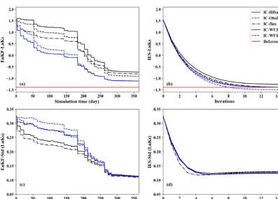
Figure 6. The results of lnKs estimations(a, b)and their associated standard deviations(c, d)within two data assimilation frameworks
(a, c: EnKF;b, d: IES) under five initialization methods (Case 1).
diversity of the meteorological condition. Since IC-ObsInt and IC-flux are created by adding observation information or simple infiltration information, they perform better than that with IC-HfSatu but worse than warm-up methods. Similarly, the assimilation results for the IES with IC-WUP are also the best, while those with IC-HfSatu have the worst parameter estimation in the five initialization methods (Fig. 6b). In ad-dition, by comparing Fig. 6a and b, the cases using the IES show better results than those using EnKF, indicating a supe-rior ability of the IES to estimate the individual parameter in variably saturated model. However, since the IES estimates parameter iteratively, it has a much larger computational cost than EnKF when using warm-up methods.
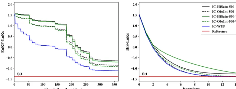
[image:10.612.101.499.224.509.2]prob-Figure 7.The impacts of increased ensemble size (Case 2) and uncertainty of initial state (Case 3) on the results of lnKsestimations within
EnKF and IES.
lem for the IES could be reduced significantly. This partly explains the inferior result of EnKF compared to the IES.
Increasing the ensemble size and model uncertainty is an efficient approach for reducing the filter inbreeding (Hen-dricks Franssen and Kinzelbach, 2008). To demonstrate the impacts of ensemble size and initial uncertainty on data as-similation results, the results of lnKs estimations utilizing the initial condition IC-HfSatu and IC-ObsInt with the en-semble size of 500 (Case 2) and a Gaussian noise (Case 3) are plotted in the Fig. 7.
The results of IC-HfSatu-500 and IC-ObsInt-500 with the ensemble size of 500 in Fig. 7 are similar to those of IC-HfSatu and IC-ObsInt (Fig. 6), indicating that the improve-ment of the parameter estimation result is slight when the ensemble size increases from 300 to 500. Hence, the ensem-ble size of 300 is sufficient for the data assimilation proensem-blem in this study. In contrast, the influences of adding the uncer-tainty to the initial state on parameter estimation are totally different for EnKF and the IES. Compared with the results of IC-ObsInt-500 and IC-HfSatu-500, the results of lnKs es-timation with IC-ObsInt-500-Un and IC-HfSatu-500-Un im-prove for EnKF (Fig. 7a) but deteriorate for the IES (Fig. 7b). This may be attributed to the diversity between two algo-rithms. EnKF is a sequential algorithm, so the state uncer-tainty introduced by the UIC could decrease over assimila-tion steps. A larger ensemble state variance implemented at the beginning leads to a larger trust in data and thus a quicker update of the parameter to truth and can prevent EnKF from inbreeding, leading to a better result than that with an ini-tial condition of small variance. On the contrary, the IES is a batch optimization method. The uncertainty of the ini-tial state exists at each iteration and has a negative effect on the model calibration during the whole simulation, worsen-ing the parameter estimation results. Besides this, we also investigate the influences of spatial correlation of the added noise (e.g., with correlation length of 50 cm or infinity) for constructing IC-HfSatu and IC-ObsInt, but their parameter estimation results are similar (not shown), indicating that the
effects of spatial correlation of noise during the construction of IC-HfSatu and IC-ObsInt are not significant in parameter estimation.
Moreover, the parameter estimation results of IC-WUP are still superior to those of HfSatu-500-Un and IC-ObsInt-500-Un even though they all have a similar compu-tational cost, showing the promising performance of warm-up methods. The results are reasonable, since all ensemble Kalman filter methods are affected by the quality of the auto-covariance matrix and the mean value of the predicted state ensemble (Eqs. 11 and 12 for EnKF; Eqs. 14 and 15 for IES). For the WUP method, the initial condition is constructed by warming up the model with the prior parameter; thus IC-WUP contains useful information of prior parameter, even it is biased. Besides this, the state covariance matrix is im-plicitly inflated due to the introduction of uncertain prior parameter ensemble during warming up. These two aspects ensure the robust performance of warm-up methods. How-ever, the initial state ensembles of IC-HfSatu-500-Un and IC-ObsInt-500-Un are independent of the prior parameter, which introduces additional uncertainties, making the data assimilation results worse. Therefore, even using a larger en-semble size and enlarging the state uncertainty (covariance inflation), warm-up methods are still the optimal choice for both EnKF and IES algorithms. We also construct another case with larger parameter uncertainty to alleviate the filter inbreeding problem, and the data assimilation for all cases are improved (not shown). The results also agree with our conclusion that WUP performs the best among the five ini-tialization methods.
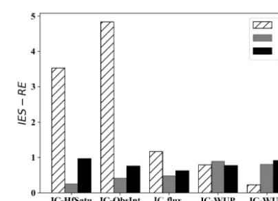
To evaluate the effects of the UIC in the multi-parameter inverse problem, the RE results ofKs,αandnestimates of Case 4 are presented in Fig. 8. In general, the RE results ofn
[image:11.612.100.498.65.216.2]Figure 8.The RE results of parameter estimations (α,nandKs) under five initialization methods with(a)EnKF and(b)IES (Case 4).
similar to the conclusion of the one-parameter inverse prob-lem, the parameter estimation results ofKs andαwith IC-HfSatu and IC-ObsInt are worse than those of IC-WUP and IC-WUE. There is not much difference between then esti-mates under various initial conditions, implying thatnis less affected by the UIC when estimating Ks,αandn simulta-neously. Compared with EnKF, the IES shows a smaller RE (Fig. 8b) for all parameters, indicating that the IES can also perform better in the multi-parameter inverse problem. How-ever, the assimilation results with various initialization meth-ods do not show much difference, implying that the final RE values are not significantly affected by the UIC, possibly due to abundant observations available over 1 year. Never-theless, long-term observation data may not be available in many cases.
To examine the impact of assimilation time on parameter estimation with the IES, Case 5 with a shorter assimilation period (60 d) and a fewer number of observations (i.e., six) is conducted. Figure 9 shows the RE results, and it is infe-rior to those in Case 4, where the simulation time is 1 year (Fig. 8b). Nevertheless, the effects of assimilation time on parameter estimation are different for different parameters. For instance, parameter ncan still be estimated well in the most of the situations. In addition, though the assimilation results ofKs degraded with a 60 d simulation, the variation inKs estimation values among different initialization meth-ods is small. The number of observations can greatly affect the estimation of parameterα, since RE values ofαin Case 5 (3.5, 4.8, 1.17, 0.79 and 0.23) are much larger than those in Case 4 (0.16, 0.29, 0.68, 0.24 and 0.31). Furthermore, the warm-up methods show the best data assimilation results among the five when the observations are insufficient.
4 Field validation
Synthetic observation in previous section is generated by running the model with uncertainty sources that are exactly known. By conducting synthetic experiments, we can thor-oughly analyze the impact of the UIC during data assimila-tion, with scenarios having different numbers of observations
Figure 9.The RE results of parameter estimations under five initial-ization methods with IES when the simulation time is 60 d (Case 5).
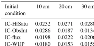
[image:12.612.325.527.233.379.2]Table 4.RMSEobsresults for the soil moisture predictions at ob-servation points with different initial conditions in the experimental case.
Initial 10 cm 20 cm 30 cm condition
IC-HfSatu 0.0232 0.0271 0.0280 IC-ObsInt 0.0286 0.0187 0.0134 IC-flux 0.0198 0.0222 0.0206 IC-WUP 0.0180 0.0153 0.0155
simulation time is also available to construct an initial profile via IC-ObsInt.
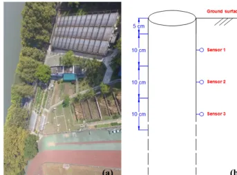
4.1 General description of the experimental case To analyze the experimental data, the 1-D numerical domain is set as 2 m and discretized in 50 grids. The top 40 grids have a size of 2.5 cm, and the rest have a size of 10 cm. The upper boundary is set as an atmospheric boundary using the data shown in Fig. 11a, and the bottom boundary is set to be free drainage, since the groundwater table is much deeper than the bottom of the domain.
The prior parameter distributions follow the study of Li et al. (2018). The saturated soil moisture θs and residual soil moistureθrare given as 0.43 and 0.078, while the other hy-draulic parameters are to be estimated. The initial means ofKs,αandnare set as 1 m d−1, 5 m−1and 2, and the initial natural logarithmic variances of them are set as 0.22, 0.16 and 0.003. The data from 18th April through 27 April are used for calibration, while the remaining data are reserved for validation. The climate of Wuhan is semi-arid condi-tions, and the soil of the experimental site is sandy loam. We use a warm-up time of 242 d based on our investigation in Sect. 3.2.2.
4.2 Results
The assimilation results with four different initialization re-sults (IC-HfSatu, IC-ObsInt, IC-flux and IC-WUP) are pre-sented in this part. Since the true hydraulic parameters at the experimental site are unknown, we assess the estima-tion by comparing the predicted (using estimated parameters) and observed soil moisture during the validation period. The RMSEobsvalues for soil moisture predictions under different assimilation scenarios are listed in Table 4. Generally speak-ing, RMSEobs values with IC-WUP are again the smallest, while IC-HfSatu has the largest RMSEobsvalues.
In order to evaluate the overall performances of the four initialization methods, the soil moisture observations and predictions at all depths are plotted in Fig. 12. The coeffi-cients of determination under the four scenarios are 0.033, 0.599, 0.083 and 0.553, and the RMSEobsvalues are 0.045, 0.037, 0.036 and 0.028, respectively. As shown in Fig. 12a
and c, IC-HfSatu and IC-flux show very large scattering, indicating a bad prediction performance. A significant im-provement is found in IC-WUP, with a large R2 and the smallest RMSEobsvalue, as shown in Fig. 12d. Surprisingly, IC-ObsInt has the largestR2among the four methods, though its RMSEobsvalue is bigger than that of IC-WUP. The simu-lation of real-world problems may have uncertainties that are not considered in data assimilation. For instance, the meteo-rological data prior to the simulation for warming up are not precise from the weather-station instrument error and calcu-lation of evapotranspiration, which has a detrimental effect on IC-WUP. IC-ObsInt, on the other hand, has the advantage of utilizing the soil moisture observations for both initializa-tion and predicinitializa-tions. However, IC-ObsInt may not be appli-cable when soil moisture observations att=0 are not avail-able or the soil moisture profile is discontinuous in layered soils, leading to a large interpolation error. In summary, for both the synthetic and field cases, models initialized using the warm-up method result in low uncertainty and superior soil moisture predictions even if the calibration data are in-sufficient.
5 Discussion and conclusions
The study investigates the effects of the UIC on variably sat-urated flow simulations subject to different soil hydraulic pa-rameters, meteorological conditions and soil profile lengths. Two common approaches (spin-up and Monte Carlo meth-ods) are applied to explore the required warm-up timetwu and temporal behavior of the UIC. In addition, the data as-similation performances with five common initialization ap-proaches are compared using synthetic experiments and a field soil moisture dataset.
Figure 10.The experimental site:(a)overhead view and(b)the cross-sectional view of the FDR sensor.
Figure 11. The meteorological information and observed soil moisture over the experimental time.(a)Observed rainfall and calculated potential evaporation.(b)Temporal change of soil moisture data at three different observed depths (10, 20 and 30 cm).
soil profile lengths, and special attention should be paid dur-ing vadose zone modeldur-ing.
Ideally, the initial ensemble should represent the error statistics of the initial guess for the model state during data assimilation (Evensen, 2003). Thus, effort should be invested in reducing the impact of the UIC on data assimilation. Meth-ods which do not consider the UIC (i.e., assuming an initial ensemble arbitrarily without uncertainty, which was used in some studies; e.g., Shi et al., 2015) can induce significant bias according to our data assimilation results. By construct-ing the initial condition usconstruct-ing the information of observa-tions or the boundary condition (averaged flux), the data as-similation results can be improved. However, these two
ini-tialization methods are also suboptimal due to the oversim-plification of the complex initial condition. By warming up the model with available meteorological data, the initializa-tion methods can improve data assimilainitializa-tion results. More-over, EnKF is more sensitive to the filter inbreeding problem than the IES. The initial condition with a larger state uncer-tainty gains better performance than that without covariance inflation for EnKF, while for the IES, this inflated uncertainty cannot decrease over iterations, making the results inferior.
[image:14.612.70.524.354.511.2]Figure 12.The comparisons between soil moisture observations and predictions (with estimated parameters from IES combined with differ-ent initialization methods) at all observation depths.
head (i.e., UIC in terms of the pressure head can be converted from that of soil moisture). The situation will be much more complex if the soil is heterogeneous, since a large number of unknown hydraulic parameters may introduce significant nonlinearity during the transformation between the head and soil moisture. For instance, the soil moisture profile is dis-continuous in layered soils. The use of the pressure head in-stead of soil moisture as the initial condition for heteroge-neous soils deserves investigation in our future work.
Our work leads to the following major conclusions: 1. The spin-up method and Monte Carlo method can both
quantify the UIC, and they agree well with each other after a sufficiently long simulation. A threshold of 0.5 % for percentage cutoff PC or ensemble spreadSpis rec-ommended to determine the warm-up time.
2. Warm-up time varies nonlinearly with soil textures, me-teorological conditions and soil profile length. Under most situations (e.g., loam with the soil profile length less than 5 m under non-arid climate), a 1-year warm-up time is sufficient for soil water movement modeling, but an extremely long time (exceeds 10 years) is needed to warm up the model for a long, fine-textured soil pro-file under an arid meteorological condition.
3. The IES shows better performance than EnKF in the strongly nonlinear problem and is affected less by the
UIC with a long period of observations. In addition, co-variance inflation of the initial condition could improve the data assimilation results for EnKF but deteriorate them for the IES.
4. The following procedure is recommended to initial-ize soil water modeling: (1) evaluate the approximate warm-up time based on the model settings, (2) initialize the model using the method of the WUP (if meteorolog-ical data are available) and make sure the warm-up time is larger than the requiredtwu, and (3) run the simula-tion with the initial condisimula-tion obtained in step 2. WUE is an alternative to WUP if the preceding meteorological data are not available. ObsInt is also a practical choice if dense soil moisture observations at the beginning of simulation are available.
Further research may examine the performance of these ini-tialization methods in two- or three-dimensional variably sat-urated flow conditions. Our approach can also be extended to other modeling and data assimilation problems in other disci-plines (e.g., groundwater flow and solute transport modeling and soil–water–crop modeling).
Author contributions. YZ and JY developed the new package for soil water flow modeling based switching the primary variable of the numerical Richards’ equation; DY and YZ developed EnKF and the IES codes for data assimilation of variably saturated flow and designed and conducted the numerical cases and field data val-idation for this study. Seven of the co-authors made non-negligible efforts in preparing the paper.
Competing interests. The authors declare that they have no conflict of interest.
Acknowledgements. This work is supported by the Natural Science Foundation of China through grant nos. 51609173, 51779179 and 51861125202. The authors appreciate Michael Tso (Lancaster Uni-versity, UK) for editing the paper. We thank the three reviewers for their constructive comments and suggestions.
Financial support. This research has been supported by the Na-tional Natural Science Foundation of China (grant nos. 51609173, 51779179 and 51861125202).
Review statement. This paper was edited by Bill X. Hu and re-viewed by Heng Dai and two anonymous referees.
References
Ajami, H., McCabe, M. F., Evans, J. P., and Stisen, S: Assessing the impact of model warm-up on surface water-groundwater interac-tions using an integrated hydrologic model, Water Resour. Res., 50, 1–21, https://doi.org/10.1002/2013WR014258, 2014. Ataie-Ashtiani, B., Volker, R. E., and Lockington, D. A.:
Numer-ical and experimental study of seepage in unconfined aquifers with a periodic boundary condition, J. Hydrol., 222, 165–184, https://doi.org/10.1016/S0022-1694(99)00105-5, 1999. Bauser, H. H., Jaumann, S., Berg, D., and Roth, K.: EnKF with
closed-eye period – Towards a consistent aggregation of informa-tion in soil hydrology, Hydrol. Earth Syst. Sci., 20, 4999–5014, https://doi.org/10.5194/hess-20-4999-2016, 2016.
Carsel, R. F. and Parrish, R. S.: Developing joint probability dis-tributions of soil water retention characteristics, Water Resour. Res., 24, 755–769, https://doi.org/10.1029/WR024i005p00755, 1988.
Castillo, V. M., Gómez-Plaza, A., and Martínez-Mena, M.: The role of antecedent soil water content in the runoff response of semi-arid catchments:A simulation approach, J. Hydrol., 284, 114– 130, https://doi.org/10.1016/S0022-1694(03)00264-6, 2003. Chanzy, A., Mumen, M., and Richard, G.: Accuracy of top
soil moisture simulation using a mechanistic model with limited soil characterization, Water Resour. Res., 44, 1–16, https://doi.org/10.1029/2006WR005765, 2008.
Chen, Y. and Oliver, D. S.: Levenberg-Marquardt forms of the iterative ensemble smoother for efficient history matching
and uncertainty quantification, Comput. Geosci., 17, 689–703, https://doi.org/10.1007/s10596-013-9351-5, 2013.
Chirico, G. B., Medina, H., and Romano, N.: Kalman filters for assimilating near-surface observations into the Richards equa-tion – Part 1: Retrieving state profiles with linear and nonlin-ear numerical schemes, Hydrol. Earth Syst. Sci., 18, 2503–2520, https://doi.org/10.5194/hess-18-2503-2014, 2014.
Cosgrove, B. A., Lohmann, D., Mitchell, K. E., Houser, P. R., Wood, E. F., Schaake, J. C., Robock, A., Sheffield, J., Duan, Q. Y., Luo, L. F., Higgins, R. W., Pinker, R. T., and Tarpley, J. D.: Land surface model spin-up behavior in the North Ameri-can Land Data Assimilation System (NLDAS), J. Geophys. Res., 108, 8845, https://doi.org/10.1029/2002JD003316, 2003. Crestani, E., Camporese, M., Baú, D., and Salandin, P.: Ensemble
Kalman filter versus ensemble smoother for assessing hydraulic conductivity via tracer test data assimilation, Hydrol. Earth Syst. Sci., 17, 1517–1531, https://doi.org/10.5194/hess-17-1517-2013, 2013.
Das, N. N. and Mohanty, B. P.: Root zone soil moisture assessment using remote sensing and vadose zone modeling, Vadose Zone J., 5, 296, https://doi.org/10.2136/vzj2005.0033, 2006.
DeChant, C. M.: Quantifying the impacts of initial condition and model uncertainty on hydrological forecasts, PhD thesis, Port-land State University, PortPort-land, USA, 2014.
DeChant, C. M. and Moradkhani, H.: Improving the characteriza-tion of initial condicharacteriza-tion for ensemble streamflow prediccharacteriza-tion us-ing data assimilation, Hydrol. Earth Syst. Sci., 15, 3399–3410, https://doi.org/10.5194/hess-15-3399-2011, 2011.
De Goncalves, L. G. G., Shuttleworth, W. J., Burke, E. J., Houser, P., Toll, D. L., Rodell, M., and Arsenault, K.: To-ward a South America Land Data Assimilation System: As-pects of land surface model warm-up using the Simpli-fied Simple Biosphere, J. Geophys. Res.-Atmos., 111, 1–13, https://doi.org/10.1029/2005JD006297, 2006.
De Lannoy, G. J., Reichle, R. H., Houser, P. R., Pauwels, V., and Verhoest, N. E.: Correcting for forecast bias in soil moisture as-similation with the ensemble Kalman filter. Water Resour. Res., 43, W09410, https://doi.org/10.1029/2006WR005449, 2007. Doussan, C., Jouniaux, L., and Thony, J. L.: Variations of
self-potential and unsatureated water flow with time in sandy loam and clay loam soils, J. Hydrol., 267, 173–185, https://doi.org/10.1016/S0022-1694(02)00148-8, 2002. Emerick, A. A. and Reynolds, A. C.: Ensemble smoother
with multiple data assimilation, Comput. Geosci., 55, 3–15, https://doi.org/10.1016/j.cageo.2012.03.011, 2013.
Erdal, D., Neuweiler, I., and Wollschläger, U.: Using a bias aware EnKF to account for unresolved structure in an un-saturated zone model, Water Resour. Res., 50, 132–147, https://doi.org/10.1002/2012WR013443, 2014.
Evensen, G.: Sequential data assimilation with a nonlinear quasi-geostrophic model using Monte Carlo methods to forecast error statistics, J. Geophys. Res.-Oceans, 99, 10143–10162, https://doi.org/10.1029/94JC00572, 1994.
Evensen, G.: The Ensemble Kalman Filter: Theoretical formula-tion and practical implementaformula-tion, Ocean Dynam., 53, 343–367, https://doi.org/10.1007/s10236-003-0036-9, 2003.
hydrology at Yucca Mountain, Nevada, J. Hydrol., 247, 1–30, https://doi.org/10.1016/S0022-1694(01)00358-4, 2001. Forsyth, P. A., Wu, Y. S., and Pruess, K.: Robust numerical
methods for saturated-unsaturated flow with dry initial condi-tions in heterogeneous media, Adv. Water Resour., 18, 25–38, https://doi.org/10.1016/0309-1708(95)00020-J, 1995.
Freeze, R. A.: The Mechanism of Natural Ground-Water Recharge and Discharge: 1. One-dimensional, Vertical, Un-steady, Unsaturated Flow above a Recharging or Discharging Ground-Water Flow System, Water Resour. Res., 5, 153–171, https://doi.org/10.1029/WR005i001p00153, 1969.
French, H. K., Van Der Zee, S. E. A. T. M., and Lei-jnse, A.: Differences in gravity-dominated unsaturated flow during autumn rains and snowmelt, Hydrol. Pro-cess., 13, 2783–2800, https://doi.org/10.1002/(SICI)1099-1085(19991215)13:17<2783::AID-HYP899>3.0.CO;2-9, 1999. Galantowicz, J. F., Entekhabi, D., and Njoku, E. G.: Tests of
sequen-tial data assimilation for retrieving profile soil moisture and tem-perature from observed L-band radiobrightness, IEEE. T. Geosci. Remote, 37, 1860–1870, https://doi.org/10.1109/36.774699, 1999.
Sellers, A., Yang, Z.-L., Dickinson, R. E., Henderson-Sellers, A., Yang, Z.-L., and Dickinson, R. E.: The project for in-tercomparison of land-surface parameterization schemes, B. Am. Meteorol. Soc., 74, 1335–1349, https://doi.org/10.1175/1520-0477(1993)074<1335:TPFIOL>2.0.CO;2, 1993.
Hendricks Franssen, H. J. and Kinzelbach, W.: Real-time groundwater flow modeling with the Ensemble Kalman Fil-ter: Joint estimation of states and parameters and the fil-ter inbreeding problem, Wafil-ter Resour. Res., 44, 1–21, https://doi.org/10.1029/2007WR006505, 2008.
Hu, S., Shi, L., Zha, Y., Williams, M., and Lin, L.: Simul-taneous state-parameter estimation supports the evaluation of data assimilation performance and measurement design for soil-water-atmosphere-plant system, J. Hydrol., 555, 812–831, https://doi.org/10.1016/j.jhydrol.2017.10.061, 2017.
Huang, C., Li, X., Lu, L., and Gu, J.: Experiments of one-dimensional soil moisture assimilation system based on en-semble Kalman filter, Remote Sens. Environ., 112, 888–900, https://doi.org/10.1016/j.rse.2007.06.026, 2008.
Huo, S., Jin, M., Liang, X., and Lin, D.: Changes of vertical ground-water recharge with increase in thickness of vadose zone simu-lated by one-dimensional variably saturated flow model, J. Earth Sci., 25, 1043–1050, https://doi.org/10.1007/s12583-014-0486-7, 2014.
Ji, S. and Unger, P. W.: Soil water accumulation under different precipitation, potential evaporation, and straw mulch conditions, Soil Sci. Soc. Am. J., 65, 442–448, https://doi.org/10.2136/sssaj2001.652442x, 2001.
Leeuwen, P. J. and Evensen, G.: Data assimilation and in-verse methods in terms of probabilistic formulation, Mon. Weather Rev., 124, 2898–2913, https://doi.org/10.1175/1520-0493(1996)124<2898:DAAIMI>2.0.CO;2, 1996.
Li, B., Toll, D., Zhan, X., and Cosgrove, B.: Improving esti-mated soil moisture fields through assimilation of AMSR-E soil moisture retrievals with an ensemble Kalman filter and a mass conservation constraint, Hydrol. Earth Syst. Sci., 16, 105–119, https://doi.org/10.5194/hess-16-105-2012, 2012.
Li, X., Shi, L., Zha, Y., Wang, Y., and Hu, S.: Data as-similation of soil water flow by considering multiple uncer-tainty sources and spatial-temporal features: a field-scale real case study, Stoch. Environ. Res. Risk A., 32, 2477–2493, https://doi.org/10.1007/s00477-018-1541-1, 2018.
Lim, Y.-J., Hong, J., and Lee, T.-Y.: Spin-up behavior of soil mois-ture content over East Asia in a land surface model, Meteorol. At-mos. Phys., 118, 151–161, https://doi.org/10.1007/s00703-012-0212-x, 2012.
Medina, H., Romano, N., and Chirico, G. B.: Kalman filters for assimilating near-surface observations into the Richards equa-tion – Part 2: A dual filter approach for simultaneous retrieval of states and parameters, Hydrol. Earth Syst. Sci., 18, 2521–2541, https://doi.org/10.5194/hess-18-2521-2014, 2014a.
Medina, H., Romano, N., and Chirico, G. B.: Kalman filters for as-similating near-surface observations into the Richards equation – Part 3: Retrieving states and parameters from laboratory evap-oration experiments, Hydrol. Earth Syst. Sci., 18, 2543–2557, https://doi.org/10.5194/hess-18-2543-2014, 2014b.
Montzka, C., Moradkhani, H., Weihermüller, L., Franssen, H. J. H., Canty, M., and Vereecken, H.: Hydraulic parame-ter estimation by remotely-sensed top soil moisture obser-vations with the particle filter, J. Hydrol., 399, 410–421, https://doi.org/10.1016/j.jhydrol.2011.01.020, 2011.
Mualem, Y.: Wetting front pressure head in the infiltration model of Green and Ampt, Water Resour. Res., 12, 564–566, https://doi.org/10.1029/WR012i003p00564, 1976.
Mumen, M.: Caractérisation du fonctionnement hydrique des sols à l’aide d’un modèle mécaniste de transferts d’eau et de chaleur mis en oeuvre en fonctions des informations disponibles sur le sol, PhD thesis, University of Avignon, Avignon, France, 2006. Oliver, D. S. and Chen, Y.: Improved initial sampling for
the ensemble Kalman filter, Comput. Geosci., 13, 13–27, https://doi.org/10.1007/s10596-008-9101-2, 2009.
Pujol, J.: The solution of nonlinear inverse problems and the Levenberg–Marquardt method, Geophysics, 72, W1–W16, https://doi.org/10.1190/1.2732552, 2007.
Rahman, M. M. and Lu, M.: Model spin-up behavior for wet and dry basins: A case study using the Xinanjiang model, Water, 7, 4256–4273, https://doi.org/10.3390/w7084256, 2015.
Reichle, R. H. and Koster, R. D.: Assessing the Im-pact of Horizontal Error Correlations in Background Fields on Soil Moisture Estimation, J. Hydrome-teorol., 4, 1229–1242, https://doi.org/10.1175/1525-7541(2003)004<1229:ATIOHE>2.0.CO;2, 2003.
Rodell, M., Houser, P. R., Berg, A. A., and Famiglietti, J. S.: Eval-uation of 10 Methods for Initializing a Land Surface Model, J. Hydrometeorol., 6, 146–155, https://doi.org/10.1175/JHM414.1, 2005.
Ross, P. J.: Modeling soil water and solute transport – fast, simplified numerical solutions, Agron. J., 95, 1352–1361, https://doi.org/10.2134/agronj2003.1352, 2003.
Seck, A., Welty, C., and Maxwell, R. M.: Spin-up be-havior and effects of initial conditions for an integrated hydrologic model, Water Resour. Res., 51, 2188–2210, https://doi.org/10.1002/2014WR016371, 2014.
unsaturated flow parameters, J. Hydrol., 524, 549–561, https://doi.org/10.1016/j.jhydrol.2015.01.078, 2015.
Šim˚unek, J., Šejna, M., Saito, H., Sakai, M., and van Genuchten, M. T.: The Hydrus-1D software package for simulating the move-ment of water, heat, and multiple solutes in variably saturated media, version 4.16, HYDRUS software series 3, Department of Environmental Sciences, University of California Riverside, Riverside, California, USA, 308 pp., 2013.
Szomolay, B.: Analysis of a moving boundary value problem aris-ing in biofilm modellaris-ing, Math. Method Appl. Sci., 31, 1835– 1859, https://doi.org/10.1002/mma.1000, 2008.
Tran, A. P., Vanclooster, M., and Lambot, S.: Improving soil mois-ture profile reconstruction from ground-penetrating radar data: A maximum likelihood ensemble filter approach, Hydrol. Earth Syst. Sci., 17, 2543–2556, https://doi.org/10.5194/hess-17-2543-2013, 2013.
van Genuchten, M. T.: A closed-form equation for predicting the hydraulic conductivity of unsatu-rated soils, Soil Sci. Soc. Am. J., 44, 892–898, https://doi.org/10.2136/sssaj1980.03615995004400050002x, 1980.
van Genuchten, M. T. and Parker, J. C.: Boundary condi-tions for displacement experiments through short labora-tory soil columns, Soil Sci. Soc. Am. J., 48, 703–708, https://doi.org/10.2136/sssaj1984.03615995004800040002x, 1984.
Varado, N., Braud, I., Ross, P. J., and Haverkamp, R.: Assessment of an efficient numerical solution of the 1D Richards’ equation on bare soil, J. Hydrol., 323, 244– 257, https://doi.org/10.1016/j.jhydrol.2005.07.052, 2006.
Vereecken, H., Huisman, J. A., Bogena, H., Vanderborght, J., Vrugt, J. A., and Hopmans, J. W.: On the value of soil moisture measure-ments in vadose zone hydrology: A review, Water Resour. Res., 46, 1–21, https://doi.org/10.1029/2008WR006829, 2010. Walker, J. P. and Houser, P. R.: A methodology for initializing soil
moisture in a global climate model: Assimilation of near-surface soil moisture observations, J. Geophys. Res.-Atmos., 106, 11761–11774, https://doi.org/10.1029/2001JD900149, 2001. Wu, C. C. and Margulis, S. A.: Feasibility of real-time soil state
and flux characterization for wastewater reuse using an embed-ded sensor network data assimilation approach, J. Hydrol., 399, 313–325, https://doi.org/10.1016/j.jhydrol.2011.01.011, 2011. Wu, C. C. and Margulis, S. A.: Real-time soil moisture
and salinity profile estimation using assimilation of em-bedded sensor datastreams, Vadose Zone J., 12, 1–17, https://doi.org/10.2136/vzj2011.0176, 2013.
Xie, T., Liu, X., and Sun, T.: The effects of groundwater table and flood irrigation strategies on soil water and salt dynamics and reed water use in the Yellow River Delta, China, Ecol. Model., 222, 241–252, https://doi.org/10.1016/j.ecolmodel.2010.01.012, 2011.
Yang, Z. L., Dickinson, R. E., Henderson-Sellers, A., and Pitman, A. J.: Preliminary study of spin-up processes in land surface models with the first stage data of Project for Intercomparison of Land Surface Parameterization Schemes Phase 1(a), J. Geophys. Res., 100, 16553, https://doi.org/10.1029/95JD01076, 1995. Zha, Y., Shi, L., Ye, M., and Yang, J.: A generalized