https://doi.org/10.5194/hess-23-351-2019 © Author(s) 2019. This work is distributed under the Creative Commons Attribution 4.0 License.
Contaminant source localization via Bayesian global optimization
Guillaume Pirot1, Tipaluck Krityakierne2,3,4, David Ginsbourger4,5,6, and Philippe Renard7 1Institute of Earth Sciences, University of Lausanne, Lausanne, Switzerland
2Department of Mathematics, Faculty of Science, Mahidol University, Bangkok, Thailand 3Centre of Excellence in Mathematics, CHE, Bangkok, Thailand
4Oeschger Center for Climate Change Research, University of Bern, Bern, Switzerland
5Uncertainty Quantification and Optimal Design group, Idiap Research Institute, Martigny, Switzerland 6Institute of Mathematical Statistics and Actuarial Science, University of Bern, Bern, Switzerland 7Centre for Hydrogeology and Geothermics, University of Neuchâtel, Neuchâtel, Switzerland Correspondence:Guillaume Pirot ([email protected])
Received: 29 June 2017 – Discussion started: 14 August 2017
Revised: 17 October 2018 – Accepted: 16 December 2018 – Published: 21 January 2019
Abstract.Contaminant source localization problems require efficient and robust methods that can account for geological heterogeneities and accommodate relatively small data sets of noisy observations. As realism commands hi-fidelity sim-ulations, computation costs call for global optimization al-gorithms under parsimonious evaluation budgets. Bayesian optimization approaches are well adapted to such settings as they allow the exploration of parameter spaces in a princi-pled way so as to iteratively locate the point(s) of global op-timum while maintaining an approximation of the objective function with an instrumental quantification of prediction un-certainty. Here, we adapt a Bayesian optimization approach to localize a contaminant source in a discretized spatial do-main. We thus demonstrate the potential of such a method for hydrogeological applications and also provide test cases for the optimization community. The localization problem is illustrated for cases where the geology is assumed to be per-fectly known. Two 2-D synthetic cases that display sharp hy-draulic conductivity contrasts and specific connectivity pat-terns are investigated. These cases generate highly nonlin-ear objective functions that present multiple local minima. A derivative-free global optimization algorithm relying on a Gaussian process model and on the expected improvement criterion is used to efficiently localize the point of minimum of the objective functions, which corresponds to the contam-inant source location. Even though concentration measure-ments contain a significant level of proportional noise, the al-gorithm efficiently localizes the contaminant source location. The variations of the objective function are essentially driven
by the geology, followed by the design of the monitoring well network. The data and scripts used to generate objective functions are shared to favor reproducible research. This con-tribution is important because the functions present multiple local minima and are inspired from a practical field appli-cation. Sharing these complex objective functions provides a source of test cases for global optimization benchmarks and should help with designing new and efficient methods to solve this type of problem.
1 Introduction
where forward runs are CPU-intensive. On the other hand, so-called Bayesian optimization algorithms have been gain-ing considerable importance in several fields lately as they enjoy a number of practical advantages while having been recently proven to possess desirable consistency properties (Vazquez and Bect, 2010; Bect et al., 2018). One of the great-est strengths of common Bayesian optimization algorithms is that they do not only guide evaluations towards the global optimum but also maintain an approximate representation of the objective function together with a quantification of pre-diction uncertainty. This enables space exploration with a memory so as to prevent or mitigate evaluations at redun-dant locations. Recent adaptations of popular Bayesian opti-mization approaches allow the accommodation of evaluation noise (Picheny and Ginsbourger, 2014), parallel evaluations (Marmin et al., 2015), high dimensions (Wang et al., 2018), nonstationarity (Snoek et al., 2014), gradient observations (Wu et al., 2017) and many more features (see for instance Ginsbourger, 2018, for a broader overview of sequential de-sign algorithms for computer experiments).
Despite the fantastic rise of Bayesian optimization in ma-chine learning and for the design of computer in various communities, its spread in the geosciences remains relatively modest so far, perhaps in part because, contrary to analytical test functions inspired by engineering problems or off-the-shelf machine learning algorithms trained on openly avail-able databases, it is often the case (e.g., in heavy-flow sim-ulations) that geoscientific data and/or computer codes can-not be publicly shared or easily handled for one or the other reason. One way around that is to share instead a finite num-ber of evaluation results performed on-site by the authors, so that users do not need to run new simulations when test-ing their algorithms. Yet, optimization algorithms typically used in hydrogeological inverse and related problems assume a continuous search space. When relying on a discretization of the input space, possible options that come to mind include (i) using discrete optimization algorithms, (ii) using contin-uous optimization algorithms on a re-interpolated function based on available evaluation results, and (iii) constraining continuous optimization methods by forcing novel evalua-tion points to remain among the considered finite set. Our approach here, guided by the willingness to share data with both geoscience and optimization communities and produce reproducible research, is to rely on a fine grid of evalua-tion results that allows any of the aforemenevalua-tioned three ap-proaches to be used.
By remaining in a two-dimensional framework, our dis-cretized 2601-element data set is actually fine enough to cap-ture the complex behavior of the misfit functions considered so that optimization algorithms can be possibly compared by users on high-fidelity approximations of the objective. That being said, we insist throughout the paper on a natural adap-tion of a popular Bayesian optimizaadap-tion algorithm to the dis-crete case, hence simultaneously addressing points (i) and (iii) above and thus demonstrating the applicability of this
family of techniques both to challenging contaminant local-ization problems in general and to discrete situations in par-ticular (that could be relevant in a number of practical situa-tions, e.g., well placement).
Coming back to more specific hydrogeological concerns underlying our application test case, contaminant character-ization problems are motivated by the fact that the concept of polluter pays (OECD, 1972) holds for groundwater pro-tection laws in many countries (USA, 1972; Swiss Confed-eration, 1983; European Union, 2000). A polluter can some-times be identified by a specific chemical signature (Man-suy et al., 1997; Rachdawong and Christensen, 1997; Venka-tramanan et al., 2016). However, when the signature is not unique, the ability to localize the contaminant source(s) can make defining responsibilities or reducing decontamination costs easier. Moreover, contaminant transport is dominated by the heterogeneity of the subsurface properties. In partic-ular, it is controlled by the connectivity of geobodies (e.g., characterized by lithofacies or by a range of hydraulic con-ductivity values) and by the sharpness of geobody property contrasts.
Within this last set of methods, different optimization tech-niques can be employed. Classical nonlinear optimization techniques following a derivative-based approach (Mahar and Datta, 2000; Datta et al., 2011), such as the Levenberg– Marquardt algorithm (Hansen and Vesselinov, 2016), present the risk of being stuck in local minima. Employing a tabu search algorithm (Yeh et al., 2007) presents the same incon-venience as it iteratively explores neighbor solutions. Com-bining a gradient descent algorithm with a genetic algorithm (Aral et al., 2001; Ayvaz, 2016) decreases the risk of becom-ing stuck in local minima, but the genetic algorithm may re-quire longer parameter exploration if the mutations are not guided by a smart rule. Simulated annealing (Amirabdol-lahian and Datta, 2014) allows for a broader exploration but at a very high computational cost. Bayesian optimization1 is a global approach that considerably limits the risk of be-ing trapped in local minima and does not require the com-putation of derivatives of the objective function. It smartly explores the parameter space by looking at figures of merit such as the expected improvement (EI) criterion (Mockus, 1989; Jones et al., 1998; Vazquez and Bect, 2010), trading off exploitation of available results and space exploration. To the best of our knowledge, the potential of this class of meth-ods for addressing contaminant source localization problems is still unexplored.
The objective of this paper is threefold.
The first objective is to assess the performance of an in-verse problem formulation to identify contaminant source characteristics on a synthetic case displaying strong hydro-geological property contrasts and complex connected struc-tures. This is important because in spite of its advantages, inverse problem formulation to identify contaminant source characteristics has been employed only on multi-Gaussian-type heterogeneities, and the multi-Gaussian-type of heterogeneities strongly influences mass transport.
The second objective is to test the efficiency and advan-tages of a Bayesian optimization algorithm which relies on expected improvement criteria in the formulated contaminant source identification problem. While Bayesian optimization has been applied to a variety of optimization problems, we believe that this is the first time the algorithm has been ap-plied to the contaminant source identification problem.
And last but not least, the third objective is to provide an open-source optimization benchmark case that allows the comparison of different optimization strategies on objective functions defined over a discrete domain and inspired by real
1While Bayesian methods have been massively used throughout
groundwater sciences and notably for contaminant source localiza-tion, let us emphasize that the term “Bayesian optimization” does not refer to any arbitrary method that combines “optimization” and “Bayesian statistics”. Instead, the term refers to a specific family of optimization algorithms where a prior distribution is put on the objective function (see for example Shahriari et al., 2016, and ref-erences therein for an overview).
applications, which are not currently available in the opti-mization community.
With these objectives, we propose an original application of an EI algorithm to infer, in a deterministic inverse prob-lem formulation, the contaminant source location in a 2-D heterogeneous aquifer that presents strong property contrasts and complex connected structures. To allow for a compar-ison between the optimizer exploration and an exhaustive search of the discrete parameter space, the model grid is lim-ited to 2-D to keep computational costs reasonable for flow and transport simulations. The hydraulic conductivity field is generated with the multiple-point statistics algorithm called DeeSse (Straubhaar et al., 2016), from a training image rep-resenting the heterogeneous hydrogeological properties of a braided-river aquifer, which was generated by a pseudo-genetic algorithm (see Appendix A; Pirot et al., 2015). The hydrogeological properties and flow boundary conditions are assumed to be perfectly known. The flow and transport equa-tions are solved numerically using the Groundwater software (Cornaton, 2007). Because the measurement error and mon-itoring network affect the objective function, the algorithm performances are tested for different levels of measurement error and for different configurations of monitoring wells. The optimization is performed using the DiceKriging and DiceOptim R packages (Roustant et al., 2012). In addition, we provide a benchmark for optimization algorithms, which relies on an objective function generator that can be cus-tomized by choosing between two geological scenarios, two possible locations for the contaminant source and by the se-lection of observations among 25 monitoring wells. The per-formance of the EI algorithm is assessed by 100 runs from different initial designs.
The paper is organized as follows. Section 2 describes the synthetic test case and the experimental setup. Section 3 ex-plains the objective function generator. Section 4 details the steps of the EI algorithm. The results are presented in Sect. 5 and are discussed in Sect. 6. Conclusions are summed up in Sect. 7. The open-source code provided online is listed in the Appendix.
2 Synthetic test cases
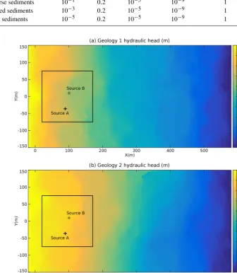
Figure 1.Experimental setup: 600 m×300 m 2-D facies model of the aquifer:(a)geology 1 and(b)geology 2. The black square delimits the possible locations for the search of the contaminant source. The two reference source locations are identified by black crosses.
facies are given in Table 1 and are inspired from analogs described in the literature (Jussel et al., 1994; Bayer et al., 2011).
Note that the contaminant spreading at the scale of this model is assumed to be mainly controlled by the geological heterogeneity. Since there is always some numerical disper-sion when solving the advection disperdisper-sion equation numeri-cally, we used the smallest possible value for the longitudinal and transverse dispersivities that would stabilize the numeri-cal problem. Another method to obtain 2-D horizontal mod-els of braided river aquifers from 3-D modmod-els would have been to vertically integrate the hydraulic conductivity field, but since this smoothes out the hydraulic conductivity, the re-sulting 2-D models present fewer contrasts and less realistic connected structures.
As boundary conditions for the flow and transport model, we impose a differential head of 2 m on the length of the model (between X= −20 m andX=580 m) and no flow on the sides (Y = −150 m and Y =150 m) parallel to the main flow direction. We assume steady-state flow conditions (Fig. 2) to run transport simulations by solving the advection
dispersion equation with the finite-element code Groundwa-ter (Cornaton, 2007).
The source of the contaminant is supposed to be unique, parameterized by the coordinates of its initial center of mass, and located within a search zone delimited by a 150 m×150 m domain whose coordinates belong to [20,170]×[−75,75]. To test the influence of the source loca-tion versus the geology, first on the misfit objective funcloca-tion and second on the ability of the proposed approach to deal with more or less complex objective functions, two reference locations (A and B) were chosen.
Source A is located at (xsA=89, ysA= −36). Source B is located at (xsB=100, ysB=10). Since surface spills usu-ally present some diffusion characteristics in their shape and can cover different geological features, the initial con-taminant mass distribution at time 0 is chosen as a multi-Gaussian distribution centered on the source location with a standard deviation (σx=2.5 m,σy=1.0 m) for a total mass
Table 1.Hydrogeological parameters.
Hydraulic Storage Molecular Longitudinal Transversal
Facies conductivity Porosity coefficient diffusion dispersivity dispersivity
K(m s−1) Ss(m−1) Dm(m2s−1) αL(m) αTh(m)
Coarse sediments 10−1 0.2 10−5 10−9 1 0.1
Mixed sediments 10−3 0.2 10−5 10−9 1 0.1
Fine sediments 10−5 0.2 10−5 10−9 1 0.1
Figure 2.Steady-state flow for(a)geology 1 and(b)geology 2. The black square delimits the possible locations for the search of the contaminant source. The two reference source locations are identified by black crosses.
breakthrough curves recorded at the well number 2, 16 and 22 are given as examples at the bottom of Fig. 3.
Real applications are always characterized by measure-ment errors. In our practical application of concentration measurements, as for chemical analysis, the errors are mainly due to data acquisition, sampling in the field, dilution proce-dure, etc. These errors can be assumed either with homo-geneous variance or with a standard deviation proportional to the noiseless measurements, e.g., with a proportionality factor supposed to be below 10 % (Ramsey and Argyraki, 1997). We denote by creal(i, t ) the actual concentration at wellsi and timet (1≤i≤25 and 1≤t≤T), i.e., the one
that corresponds with the observed concentrationcobs(i, t )in the noiseless case. Now, forcobs, let us assume in the present noisy case that measurements are corrupted with a propor-tional Gaussian noise, so that observed concentrations be-come random with
cobs(i, t )=creal(i, t )×(1+κ ε(i, t )), (1) whereε(i, t )are independent and identically distributed from
N(0,1)andκ is a constant such that the level of errors does not exceed a certain proportion.
Figure 3.Misfit objective function settings:(a)location of the search zone (grey area), of the two reference contaminant sources and of the 25 groundwater monitoring wells (denoted by a circle or a triangle) within the hydrogeological model boundaries. The blue dot denotes the trial location of the contaminant;(b),(c)and(d)misfit components at wells 2, 16 and 22 respectively, resulting from the comparison of the concentration breakthrough curves simulated at the trial location with the recorded ones for reference source A.
concentration level obtained at (i, t )when the contaminant source is located at x. The aim is to find the value(s) forx that minimize(s) the following misfit objective function:
f (x)= 25 X
i=1
T
X
t=1
|cobs(i, t )−csim(x, i, t )|p !p1
, (2)
which corresponds to the `p distance between the matrices (cobs(i, t ))i∈{1,...,25},t∈{1,...,T} and (csim(x, i, t ))i∈{1,...,25},t∈{1,...,T}, where p≥1 is a pa-rameter that can be arbitrarily chosen by the modeler (in our experiments both p=1 andp=2 were considered, as mentioned later). At the location of the reference source, the function reaches its minimum. In this synthetic study, we neglect conceptual or numerical errors incsimthat may result from an incomplete knowledge of the hydraulic conductivity field or boundary conditions, which would be important to consider in a real field application.
The search zone is restricted to a discrete domainZ, us-ing a regular grid of 3 m resolution for three reasons. First, in practical applications, the location of the source is often restricted to an area thanks to historical information about in-dustrial activities or accidents. Here, we apply the same
3 Benchmark case generator
An ensemble of time-varying concentrations at 25 observa-tion wells is provided at a full factorial design of candidate points in the search zoneZ, as well as at contaminant source location B (source location A belongs to the factorial design), for two geological geometries. Allowing any combination of observation wells among the 25, or any source location among the full factorial design, leads to 22×2602×(225−1) possible test functions (i.e., more than 349×109test cases). Moreover, any customized source of error can be added in the generation of the objective function. As these functions are known through their respective 512 values at the dis-cretized source spaceZ, they can be re-interpolated (e.g., us-ing splines) for continuous optimization purposes. Here we instead consider the discrete problem of selecting the optimal location among 512candidates and for that goal, we will ap-ply a straightforward discretized version of an EI algorithm as presented in the next section. The data and some R func-tions to generate benchmarks for any input parameters are provided on GitHub at https://github.com/gpirot/BGICLP (Pirot, 2018). A brief description of the repository is given in Appendix B of this paper.
4 Optimization methodology
The optimization algorithm used hereafter to minimizef (x) over the domain uses a machine learning approach relying on Gaussian process (GP) models (Rasmussen and Williams, 2006) to improve iteratively the knowledge off (x)over the domain. It is indeed based on the iterative evaluation off (x) at locations whose potential to improve the minimum among the evaluated objective function at previously explored loca-tions is the greatest. The following steps give an overview of the proposed algorithm. In what follows, more details are given about the required assumptions, the way to estimate f (x)and the definition of the expected improvement crite-rion.
The algorithm belongs to a class of Bayesian optimiza-tion algorithms (Mockus, 1989; Shahriari et al., 2016). The Bayesian aspect refers to placing a random process priorY on the unknown functionf (possibly computationally expen-sive) and updating its probability distribution thanks to avail-able evaluation results. The optimization part relies on us-ing conditional distributions ofY to iteratively choose points with the identification of f’s global optimum and/or op-timizer(s) in view. The crux is to fit adequate probabilis-tic models and also to design adapted acquisition functions (a.k.a. infill sampling criteria in surrogate-based optimiza-tion) in order to drive algorithms to an efficient optimization. GPs constitute a very popular class of probabilistic models that are fully specified by a mean functionm (x)and a covari-ance functionk x,x0(Rasmussen and Williams, 2006). In this work, we use ordinary kriging with a Matérn (ν=3/2)
Algorithm 1 Optimization algorithm overview; n0 is the number of initial locations used to define the initial knowl-edge;N is the budget, or the number of time the objective function can be evaluated;ncounts the number of times that the objective function has been evaluated.
Knowledge initialization: evaluatef (x)atn0initial locations
defined by an initial design Setn=n0
whilen≤Ndo
Based on the current knowledge, compute the expected im-provement criterion EIn(x)over the domain
Evaluatef (x)where EIn(x)is maximum
Increment the knowledge andn end while
Return the location wheref (x)is minimum over the evaluated locations
covariance function (see Roustant et al., 2012, for details) and the covariance parameters are estimated by maximum likelihood using the DiceKriging R package. While it is also possible to use a transformation of the response in GP-based optimization (e.g., Jones et al., 1998), on the considered data it did not lead to substantial differences in optimization per-formance despite the non-negativity of the misfit.
Denoting training inputs and outputs as Xn=
(x1,x2, . . .,xn) and fn=(f (x1) , f (x2) , . . ., f (xn))
and assuming a GP prior with a constant unknown mean (endowed with an improper uniform prior) leads to a Gaus-sian conditional distribution with the following marginal predictive mean and variance:
mn(x)= ˆµ+k(x)TK−1(fn− ˆµ1), (3)
sn2(x)=k(x,x)−k(x)TK−1k(x) +(1−k(x)
TK−11)2
1TK−11 , (4)
whereK=(k(xi,xj))i,j=1,...,nis then×nprior covariance
matrix (assumed invertible here) of responses at training in-puts,k(x)=(k(x,x1), . . ., k(x,xn))T is ann×1 covariance
vector andµˆ=1TK−1fn
1TK−11 is the best linear unbiased estimate
ofµ.
The optimization algorithm typically starts with construct-ing a space-fillconstruct-ing designXn0=(x1,x2, . . .,xn0)(see, e.g.,
Dupuy et al., 2015) and evaluatingf Xn0
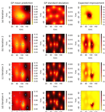
to initialize the knowledge of the algorithm (e.g.,n0=9 blue dots in the left panel of Fig. 4a). Here the initialXn0 is generated based on
Latin hypercube sampling (McKay et al., 1979). Then, the al-gorithm begins its iterations. In each iteration, the ensemble of n available evaluations fn=(f (x1) , f (x2) , . . ., f (xn))
the decision space how much the objective function value may be decreased relative tofmin=minfn, in expectation of
the following: EIn(x)=En
max(0, fmin−Y (x)). (5) The EI criterion offers a good balance between exploitation of regions with low predictive mean values and exploration of regions with high predictive variance, which provides an efficient optimization search scheme (e.g., red dot in the right panel of Fig. 4a). It turns out that EI can be calculated ana-lytically (Mockus, 1989; Jones et al., 1998). In our discrete settings with moderate number of search points, the EI can be computed at all unevaluated locations off (e.g., right pan-els of Fig. 4). The decision space location with the largest EI value is considered as the next pointxn+1 (e.g., red dot on right panels of Fig. 4) to evaluatef.
The optimization is run using the DiceKriging and DiceOptim R packages developed by Roustant et al. (2012). The number of iterations is fixed in advance (91 in what fol-lows) so that it stops when the maximum number of iterations allowed is reached. Covariance parameters are updated after each iteration by maximum likelihood estimation.
5 Results
The results for both the noiseless and noisy cases are pre-sented in this section. The main results are prepre-sented in Sect. 5.1. They rely on using information from all wells, and on noiseless concentration observations for the four con-figurations engendered by two geological scenarios and two possible sources of contaminant. For completeness, the al-gorithm sensitivity analysis with the noise added to the ob-jective function and with various well configurations are pre-sented in Sect. 5.2.
Note that with an initial space-filling design ofn0=9 ele-ments, and a number of iterations of 91, we define here a total budget ofN=100 evaluations of the objective function. 5.1 Main results for noiseless cases
Using information from the 25 observation wells, the opti-mization algorithm is applied over four configurations that depend on the retained geology and on the contaminant source location as described in Table 2, where the noise level κ (of Eq. 1) is set to 0 and the parameterpof the objective functionf (x)is set to 2.
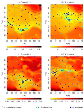
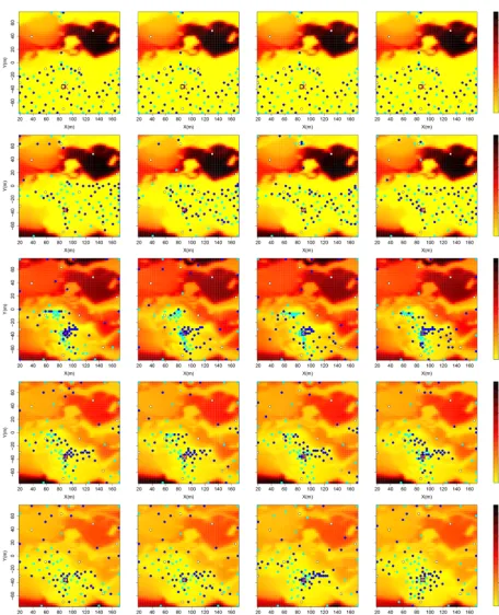
Starting from a specific initial design, the explorations of the objective functions by the EI algorithm (aiming at the contaminant source localization) are displayed in Fig. 5 for each scenario.
[image:8.612.338.518.85.153.2]These objective functions display multiple local minima, narrow valleys and sometimes very flat bottoms. These char-acteristics make the search for the global minimum challeng-ing, especially for gradient-based techniques. The locations
Table 2.Description of the four configurations.
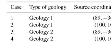
Case Type of geology Source coordinate
1 Geology 1 (89,−36)
2 Geology 1 (100,10)
3 Geology 2 (89,−36)
4 Geology 2 (100,10)
explored by the EI algorithm are plotted over the 3 m×3 m discretization of the objective functionf. The white and blue dots represent respectively the initial and then explored lo-cations where the objective function is evaluated by the al-gorithm. In most cases, the minimum of the discretized ob-jective function is reached in less than 50 evaluations. The geology seems to be the dominating factor for the global pat-terns of the objective function. Note that for scenarios 2 and 4, the contaminant source is located at (100,10), which is not within the discretized grid of the objective function; the closest point on the discretized grid is(101,9). For scenario 2, the minimum of the objective function is less than 3 m apart from the reference source located at(100,10). How-ever, for scenario 4, the reference source located at(100,10) and the minimum of the objective function located at(80,18) are 25 m apart.
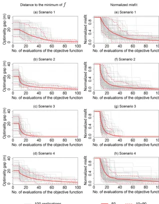
The performance of the optimization algorithm is assessed on 100 runs of the algorithms. Each run is characterized by a specific and uniformly drawn 9-point initial design. Each run is allowed a total budget of 100 evaluations of the ob-jective function. The performance depends on the number of iterations required to locate the minimum of the objective function min
x f (x). The performance can be assessed directly
by looking at the optimality gap, i.e., the distance between the location of the best estimated minimumfminof the ob-jective function and the location of its minimum min
x f (x)
as a function of the number of evaluations off (Fig. 6a–d). Another possibility is to look at the normalized best mini-mum misfit found between the true minimini-mum min
x f (x)and
Figure 4.Illustration of the first four EI algorithm iterations for scenario 1: the sub-figures in the left column illustrate the prediction mean off over the two-dimensional decision space at each iteration; the blue dots indicate the decision space locations wheref was previously evaluated; the sub-figures in the center column illustrate the prediction variance of f over the two-dimensional decision space at each iteration; the sub-figures in the right column illustrate the expected improvement map over the two-dimensional decision space at each iteration; the red dot denotes the decision space location with the maximum EI value.
5.2 Sensitivity of the algorithm performances to errors and to well configuration
In what follows, we show the results of a joint sensitivity analysis of the algorithm performance to proportional mea-surement errors and to the number of wells retained in the computation of the objective function. Four levels of propor-tional measurement errors are tested: 0 %, 10 %, 20 % and 40 %. Seven well configurations with 1, 3, 5, 10, 15, 20 or 25 wells are tested. The identification of the wells for each configuration is given in Table 3.
The cross-joint sensitivity analysis is then composed of 28 scenarios. The resulting objective functions are illustrated in Fig. D1. One can note that the precision becomes finer around the true minimum of the objective function, when increasing the number of wells. However, the improvement is limited once a line of five wells, orthogonal to the main
Table 3.Description of the seven well configurations.
Number of Well ID
wells
1 13
3 11,13,15
5 11,12,13,14,15
10 11,12,13,14,15,1,2,3,4,5
15 11,12,13,14,15,1,2,3,4,5,21,22,23,24,25 20 11,12,13,14,15,1,2,3,4,5,21,22,23,24,25,6,7,8,9,10
25 1 to 25
[image:9.612.308.547.533.645.2]uni-Figure 5.Solution exploration results for the four scenarios over the cost functions:(a, b)for geology 1;(c, d)for geology 2;(a, c)for initial contaminant location at(89,−36);(b, d)for contaminant initial location at(100,10).
formly drawn nine-point initial design. Each run is allowed a total budget of 100 evaluations of the objective function. The optimality gaps, showing the performance of the algorithm for the 28 scenarios, are displayed in Fig. D2. The optimality gap is improved with an increasing number of wells (until a full column of wells is used) and not affected by concentra-tion measurement errors.
6 Discussion
Through successive kriging of the misfit between simulated and observed concentrations, guided by the expected im-provement criterion, the proposed optimization algorithm lo-calizes efficiently the source of a contaminant in a 2-D geo-logical environment representing realistic patterns and
prop-erty contrasts. The algorithm requires approximately 50 eval-uations of the objective function in comparison to more than 2600 for an exhaustive evaluation of the discretized search zone (∼1.9 %). The total number of candidate points would increase exponentially in the number of dimensions of the parameter space, eliminating exhaustive search as an option, from even moderate dimensions, when assuming a high res-olution.
[image:10.612.140.456.63.478.2]Figure 6.Performances of the EI optimization algorithm as a function of number of evaluations of the objective function for 100 different initial design:(a, b, c, d)distance of the best solution to the location of the objective function minimum;(e, f, g, h)normalized misfit;
(a, e)scenario 1;(b, f)scenario 2;(c, g)scenario 3;(d, h)scenario 4.
an objective functionf computed withp=2, which corre-sponds to an `2 distance between reference and candidate concentration values (see Eq. 2). As the choice of p may substantially influence the flat or deep aspect of valleys (low value zones) of the objective function, we additionally tested the EI algorithm on the four scenarios for objective functions withp=1. We found that building f onto the`2 distance leads to flatter wide valleys of low values for the objective functions, which might not favor the efficiency of the EI op-timizer. However, the results and performances of the EI al-gorithm are very similar between the two norms tested. This is why we decided not to show the results of the algorithm objective functions built upon the`1distance.
When proportional measurement errors do not exceed 10 %, 20 %, 30 % or 40 %, the objective function is
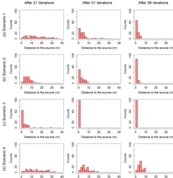
Figure 7.Distance to the contaminant source distribution for 100 runs for the best solution given by the EI algorithm: row(a)to(d)for scenarios 1 to 4.
An interesting result is that the number and configuration of wells has a strong impact on the objective function until a “full” line of wells, orthogonal to the main flow direction, is used. Increasing the number of wells on an axis orthogonal to the main flow direction greatly improves the characteriza-tion of the objective funccharacteriza-tion, notably around the true con-taminant source. It confirms what is often done in practice to catch contaminant plumes. Adding another line of obser-vation wells seems less promising than densifying a column of wells. Of course, densification might be limited in practice by minimum distances between wells to avoid connecting ar-tificially separated flowpaths for instance, but depending on the level of site characterization, a similar algorithm could then be used to optimize well configurations.
By making the source code of the objective function gen-erator available for public use, we provide several benchmark objective functions. These are driven by real hydrogeological applications and can be used for testing and comparing op-timization techniques. This benchmark will fill a gap for the community of applied mathematicians and statisticians who
Strong assumptions have been made to localize the con-taminant source in the presented application. The hydro-geolological properties and the flow boundary conditions are assumed to be perfectly known and the hydrogeologi-cal model is spatially limited to two dimensions. This al-lowed comparison of the outcome and efficiency of the algo-rithm with respect to a full grid search of the objective func-tion. Because of their expensive computing costs to assess the objective function at one location of the parameter space, three-dimensional applications will not allow for an exhaus-tive search of the solution; this is why they may require, in the near future, optimization algorithms such as the one pro-posed in this paper. Further research should also consider the uncertainty related to hydrogeological property characteriza-tion and flow and transport boundary condicharacteriza-tions. Some steps have already been made in that direction (Koch and Nowak, 2016), but were limited to common multi-Gaussian conduc-tivity fields. In addition, a regular grid discretization might compromise the ability to accurately locate the contaminant source in the presence of a strong flow path. For example, in a real-world application, the contaminant source has a very low probability of being located on a grid node. This problem could be avoided by using adaptive meshing, which would require more computing resources.
7 Conclusions
The use of 2-D hydraulic conductivity fields that present sharp contrasts and specific connectivity patterns produces complex objective functions with multiple local minima. The proposed benchmark tool produced from these complex functions offers a challenging real-world test for developers of optimization algorithms. The EI algorithm used in this 2-D study localized efficiently the contaminant source that is lo-cated on a grid node. More generally, the proposed algorithm is an interesting approach for combinatorial optimization al-gorithm. The objective functions and the performance of the algorithms are not affected by proportional measurement er-rors lower than 10 % (even 40 %). The objective function is strongly determined by the geology and by the monitoring well configuration (number and location). In particular, the characterization of the objective function, on which the per-formance of the algorithm rely, is greatly improved when a line of monitoring wells orthogonal to the main flow di-rection is densified. To improve the limitation imposed by a source centered on the nodes of a fixed mesh, which is inde-pendent of the optimization algorithm, future research could be conducted on optimization embedding adaptive meshing in flow and transport simulations; another possibility would be to relax the constraint on mass distribution of the initial plume as a way to deal with its related uncertainty. The effec-tive performance of the algorithm on this 2-D case is an en-couraging development toward 3-D applications and toward
integration of geological uncertainty in contaminant source localization problems.
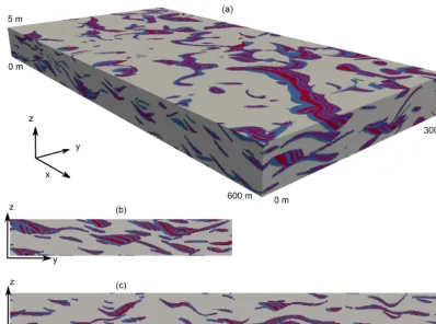
Appendix A: Training image
Appendix B: Open-source code
The electronic open-source code provided on the GitHub repository at https://github.com/gpirot/BGICLP (Pirot, 2018) with this paper contains three folders and two R scripts.
The “data” folder contains (1) the simulated concentration csim(i, t )and the actual concentrationscreal(i, t )overZand the contaminant source locations A and B ati=1,· · ·,25 ob-servation wells for the 2 geologies, and (2) thexcoordinates of the search zoneZand of the contaminant source locations A and B.
The “figures” folder contains illustrations of f (x) over Z for each of the four configurations when considering the 25 wells with the`2norm.
The “src” folder contains four R scripts. The “im-age.scale.R” script is used for graphic illustration purposes. The “generate_lhs_on_grid.R” script allows the generation of initial point designs by Latin hypercube sampling. The “functionAddNoise.R” script defines the measurement error to apply. The “functionGenerator.R” script takes as argu-ments a selection of observation wellsW, a type of geology, the source coordinates and the type of norm used. It produces the evaluation of the objective function f (x), as defined in Eq. (2).
The “plotGeneratedFunction.R” script illustrates the use of the function generator and saves the plot in the “figures” folder. The “runEGO.R” script gives an example of how to use the proposed optimization algorithm.
Appendix C: General form of error integration in the objective function
More generally, for cobs, one might assume that measure-ments are corrupted with a Gaussian noise with variance σ (i, t ) that may depend on both the welli and the time t, so that observed concentrations become random with cobs(i, t )=creal(i, t )+σ (i, t )ε(i, t ), (C1) whereε(i, t )∼N(0,1). Here for the sake of brevity we as-sume that theε(i, t )are independent for different(i, t )pairs, but the following can be extended without major difficulty to the case of correlated normals with prescribed correlation matrix.
Note that from the additive formulation above, a multiplicative noise setting can be obtained by taking σ (i, t ) to be proportional to creal(i, t ). Imposing for in-stance σ (i, t )=creal(i, t ), one indeed obtains cobs(i, t )= creal(i, t )(1+ε(i, t )).
Let us now focus on the effect of noise on the objec-tive function, and consider for simplicity the squared mis-fit in the casep=2, which becomes a random function de-noted henceforth byfε2whilef2stands for the deterministic
squared misfit from the noiseless case. We then have
fε2(x)= 25 X
i=1
T
X
t=1
(cobs(i, t )−csim(x, i, t ))2 (C2)
=
25
X
i=1 T
X
t=1
(creal(i, t )+σ (i, t )ε(i, t )−csim(x, i, t ))2 (C3)
=f2(x)+ 25 X
i=1
T
X
t=1
σ (i, t )2ε(i, t )2+2 25 X
i=1
T
X
t=1 σ (i, t )
(creal(i, t )−csim(x, i, t )) ε(i, t ). (C4) A first important note following the expansion above is that the second term, i.e.,P25i=1PT
t=1σ (i, t )2ε(i, t )2, does not depend onx so that ignoring it would not affect the behav-ior of optimization algorithms unless they are sensitive to a global shift (e.g., because of tuning parameters or stopping rules that would depend on the actual values and not solely on relative ones). In our case such a shift is not detrimental, and can even mitigate the potential issue of predicting negative misfits when using GP models without response transforma-tion. For information and, up to a multiplicative constant, the statistical distribution of this shift belongs to the generalized chi-square family (and to the usual chi-square family in the case of homogeneousσ). On the other hand, the last term of Eq. (C2) does depend both onx and on the noiseε. Denot-ingηx=2P25i=1
PT
t=1σ (i, t ) (creal(i, t )−csim(x, i, t )) ε(i, t ), it is then easy to show thatηdefines a centered Gaussian ran-dom field indexed byxin the search domainZ, and that the covariance kernel ofηboils down to the following:
Cov(ηx, ηx0)=4
25 X
i=1
T
X
t=1
σ (i, t )2(creal(i, t )−csim(x, i, t )) creal(i, t )−csim(x0, i, t ). (C5) In other words, in cases like here whencrealis actually known and experiments are run for benchmarking purposes, it is possible to propagate the effect of noise corruption on the objective function without needing to appeal to the whole set ofcsimvalues at all times and wells, but rather to a precalcu-lable covariance matrix from which the error affectingf over the grid search can be simulated. Denoting byAxthe 25×T
matrix of generic entry (2σ (i, t ) (creal(i, t )−csim(x, i, t ))) and by j a vector of ones in dimension j≥1, the
co-variance kernel of η can be written in compact form as Cov(ηx, ηx0)= 0
Appendix D: Sensitivity to concentration measurement errors and to the number of monitoring wells
Author contributions. The idea of this paper emerged from discus-sions between GP, DG, TK and PR. The hydrogeological test cases were designed by GP, with the contribution of PR. Statistical and optimization developments where mainly handled by TK and DG. Code implementation and run were performed by TK and GP. The paper was written by GP, with strong contributions from DG, TK and PR.
Competing interests. The authors declare that they have no conflict of interest.
Acknowledgements. The authors would like to thank Fabien Cornaton for his support in the parameterization and use of Groundwater, Emily Voytek and Andrew Greenwood for their support in improving the paper, and the anonymous reviewers and the editor Bill Hu for their comments and support. Tipaluck Krityakierne would like to acknowledge support from the Oeschger Center for Climate Change Research (University of Bern), the Swiss Government Excellence Scholarship, as well as the Thailand Research Fund (MRG6080208).
Edited by: Bill X. Hu
Reviewed by: three anonymous referees
References
Ababou, R., Bagtzoglou, A. C., and Mallet, A.: Anti-diffusion and source identification with the ’RAW’ scheme: a particle-based censored random walk, Environ. Fluid Mech., 10, 41–76, 2010. Ala, N. K. and Domenico, P. A.: Inverse analytical techniques
ap-plied to coincident contaminant distributions at Otis Air Force Base, Massachusetts, Groundwater, 30, 212–218, 1992. Alapati, S. and Kabala, Z.: Recovering the release history of
a groundwater contaminant using a non-linear least-squares method, Hydrol. Process., 14, 1003–1016, 2000.
Amirabdollahian, M. and Datta, B.: Identification of contaminant source characteristics and monitoring network design in ground-water aquifers: an overview, Journal of Environmental Protec-tion, 4, 23–41, 2013.
Amirabdollahian, M. and Datta, B.: Identification of pollutant source characteristics under uncertainty in contaminated water resources systems using adaptive simulated anealing and fuzzy logic, International Journal of GEOMATE, 6, 757–763, 2014. Aral, M. M., Guan, J., and Maslia, M. L.: Identification of
contam-inant source location and release history in aquifers, J. Hydrol. Eng., 6, 225–234, 2001.
Atmadja, J. and Bagtzoglou, A. C.: State of the art report on mathe-matical methods for groundwater pollution source identification, Environ. Forensics, 2, 205–214, 2001.
Ayvaz, M. T.: A hybrid simulation–optimization approach for solv-ing the areal groundwater pollution source identification prob-lems, J. Hydrol., 538, 161–176, 2016.
Bayer, P., Huggenberger, P., Renard, P., and Comunian, A.: Three-dimensional high resolution fluvio-glacial aquifer analog – Part 1: Field study, J. Hydrol., 405, 1–9, 2011.
Bect, J., Bachoc, F., and Ginsbourger, D.: A supermartingale ap-proach to Gaussian process based sequential design of experi-ments, Bernoulli, accepted, 2018.
Cornaton, F. J.: Ground water: a 3-D ground water and surface wa-ter flow, mass transport and heat transfer finite element simulator, reference manual, University of Neuchâtel, Neuchâtel, Switzer-land, 2007.
Datta, B., Chakrabarty, D., and Dhar, A.: Identification of unknown groundwater pollution sources using classical optimization with linked simulation, J. Hydro-Environ. Res., 5, 25–36, 2011. De Marsily, G.: Quantitative hydrogeology, Academic Press, Paris
School of Mines, Fontainebleau, France, 1986.
Dupuy, D., Helbert, C., and Franco, J.: DiceDesign and DiceEval: Two R Packages for Design and Analysis of Computer Experi-ments, J. Stat. Softw., 65, 1–38, 2015.
European Union: Good-quality water in Europe (EU Water Directive), available at: https://www.epa.gov/laws-regulations/ summary-clean-water-act (last access: 14 January 2019), 2000. Ginsbourger, D.: Sequential Design of Computer
Ex-periments, pp. 1–9, American Cancer Society, https://doi.org/10.1002/9781118445112.stat08124, 2018. Hansen, S. K. and Vesselinov, V. V.: Contaminant point source
lo-calization error estimates as functions of data quantity and model quality, J. Contam. Hydrol., 193, 74–85, 2016.
Jones, D., Schonlau, M., and Welch, W.: Efficient Global optimiza-tion of Expensive Black-Box Funcoptimiza-tions, J. Global Optim., 13, 455–492, 1998.
Jussel, P., Stauffer, F., and Dracos, T.: Transport modeling in hetero-geneous aquifers: 1. Statistical description and numerical gen-eration of gravel deposits, Water Resour. Res., 30, 1803–1817, 1994.
Koch, J. and Nowak, W.: Identification of contaminant source architectures-A statistical inversion that emulates multiphase physics in a computationally practicable manner, Water Resour. Res., 52, 1009–1025, 2016.
Mahar, P. S. and Datta, B.: Identification of pollution sources in transient groundwater systems, Water Resour. Manag., 14, 209– 227, 2000.
Mansuy, L., Philp, R. P., and Allen, J.: Source identification of oil spills based on the isotopic composition of individual compo-nents in weathered oil samples, Envir. Sci. Tech. Lib., 31, 3417– 3425, 1997.
Marmin, S., Chevalier, C., and Ginsbourger, D.: Differentiating the multipoint Expected Improvement for optimal batch design, in: Machine Learning, optimization, and Big Data, edited by: Parda-los, P., Pavone, M., Farinella, G., and Cutello, V., no. 9432 in Lecture Notes in Computer Science, 37–48, Springer Interna-tional Publishing, 2015.
McKay, M. D., Beckman, R. J., and Conover, W. J.: A Comparison of Three Methods for Selecting Values of Input Variables in the Analysis of Output from a Computer Code, Technometrics, 21, 239–245, 1979.
Milnes, E. and Perrochet, P.: Simultaneous identification of a sin-gle pollution point-source location and contamination time under known flow field conditions, Adv. Water Resour., 30, 2439–2446, 2007.
sur-rogate modeling for solving inverse problems, Environ. Foren-sics, 13, 348–363, 2012.
Mockus, J.: Bayesian Approach to Gobal optimization, vol. 37, Kluwer Academic Pub, Springer, the Netherlands, 1989. OECD: Guiding Principles Concerning International Economic
Aspects of Environmental Policies, Recommendation, available at: http://acts.oecd.org/Instruments/ShowInstrumentView.aspx? InstrumentID=4&InstrumentPID=255&Lang=en&Book= (last access: 14 January 2019), c(72)128, reprinted in 11 I.L.M. 1172, 1972.
Picheny, V. and Ginsbourger, D.: Noisy kriging-based optimization methods: a unified implementation within the DiceOptim pack-age, Comput. Stat. Data An., 71, 1035–1053, 2014.
Picheny, V., Wagner, T., and Ginsbourger, D.: A benchmark of kriging-based infill criteria for noisy optimization, Struct. Multi-discip. O., 48, 607–626, 2013.
Pirot, G.: gpirot/BGICLP v1.0, Benchmark Genera-tor Inspired by Contaminant Localization Problem, https://doi.org/10.5281/zenodo.2476286, 2018.
Pirot, G., Straubhaar, J., and Renard, P.: Simulation of braided river elevation model time series with multiple-point statistics, Geo-morphology, 214, 148–156, 2014.
Pirot, G., Straubhaar, J., and Renard, P.: A pseudo genetic model of coarse braided-river deposits, Water Resour. Res., 51, 9595– 9611, 2015.
Rachdawong, P. and Christensen, E. R.: Determination of PCB sources by a principal component method with nonnegative con-straints, Envir. Sci. Tech. Lib., 31, 2686–2691, 1997.
Ramsey, M. H. and Argyraki, A.: Estimation of measurement un-certainty from field sampling: implications for the classification of contaminated land, Sci. Total Environ., 198, 243–257, 1997. Rasmussen, C. E. and Williams, C. K. I.: Gaussian Processes for
Machine Learning, MIT Press, Cambridge, Massachusetts, 2006. Rios, L. M. and Sahinidis, N. V.: Derivative-free optimization: a re-view of algorithms and comparison of software implementations, J. Global Optim., 56, 1247–1293, 2013.
Roustant, O., Ginsbourger, D., and Deville, Y.: Dicekriging, Diceoptim: Two R packages for the analysis of computer experi-ments by kriging-based metamodelling and optimization, J. Stat. Softw., 51, p. 54, 2012.
Shahriari, B., Swersky, K., Wang, Z., Adams, R., and de Freitas, N.: Taking the human out of the loop: A review of bayesian op-timization, P. IEEE, 104, 148–175, 2016.
Skaggs, T. H. and Kabala, Z.: Recovering the history of a ground-water contaminant plume: Method of quasi-reversibility, Water Resour. Res., 31, 2669–2673, 1995.
Snoek, J., Swersky, K., Zemel, R., and Adams, R.: Input Warping for Bayesian optimization of Non-stationary Functions, Proceed-ings of the 31 st International Conference on Machine Learning, Beijing, China, 2014.
Straubhaar, J., Renard, P., and Mariethoz, G.: Conditioning multiple-point statistics simulations to block data, Spat. Stat.-Neth., 16, 53–71, 2016.
Swiss Confederation: Federal Act on the Protection of the Environment, available at: https://www.admin.ch/opc/en/ classified-compilation/19830267/index.html (last access: 14 January 2019), 1983.
USA: Clean Water Act, available at: https://www.epa.gov/ laws-regulations/summary-clean-water-act (last access: 14 Jan-uary 2019), 1972.
Vazquez, E. and Bect, J.: Convergence properties of the expected improvement algorithm with fixed mean and covariance func-tions, J. Stat. Plan. Infer., 140, 3088–3095, 2010.
Venkatramanan, S., Chung, S. Y., Kim, T. H., Kim, B.-W., and Selvam, S.: Geostatistical techniques to evaluate groundwater contamination and its sources in Miryang City, Korea, Environ. Earth Sci., 75, 1–14, 2016.
Wang, Z., Gehring, C., Kohli, P., and Jegelka, S.: Batched Large-scale Bayesian optimization in High-dimensional Spaces, Pro-ceedings of the 21st International Conference on Artificial Intel-ligence and Statistics (AISTATS), Lanzarote, Spain, 2018. Wu, J., Poloczek, M., Wilson, A., and Frazier, P.: Bayesian
opti-mization with Gradients, 31st Conference on Neural Information Processing Systems (NIPS 2017), Long Beach, CA, USA, 2017. Yeh, H.-D., Chang, T.-H., and Lin, Y.-C.: Groundwa-ter contaminant source identification by a hybrid heuristic approach, Water Resour. Res., 43, W09420, https://doi.org/10.1029/2005WR004731, 2007.