Does trade promote peace? squared: a gravity equation in a rectangular panel world

Munich Personal RePEc Archive

Does trade promote peace? squared: a

gravity equation in a rectangular panel

world

Parlow, Anton

University of Wisconsin-Milwaukee

31 November 2011

Online at

https://mpra.ub.uni-muenchen.de/36430/

Does Trade promote Peace? Squared: A gravity

equation in a rectangular panel world

Anton Parlow

November 2011

Abstract

The purpose of this paper is to revisit the question if trade promotes

peace or not? I account for heterogeneity of trade dyads over time in

using panel estimation techniques. The world is modeled as a rectangle.

I present models focusing on how conflict affects trade, and in another

set of models how trade affects conflict. To account for simultaneity I

use past values of trade and conflict, as well an instrumental variable

ap-proach. My instruments to explain conflict are military expenditures and

a military capability index. The instrumental variable to explain trade is

annual rainfall. I find in most setups that trade and interstate conflict

are reciprocal. Trade indeed promotes peace because of welfare gained

from international trade. Past values of conflict or trade have a negative

impact in their respective models. Only after accounting for endogeneity

in using an instrumental variable approach, the negative relationship

be-comes insignificant or positive in some setups. I employ a dynamic panel

estimator to deal with possible limitations of the instrumental variables.

JEL-Classification: F14, 019, N40

Keywords: Trade, Conflicts, GDP, Gravity model

∗_{Doctoral Student, Department of Economics, University of Wisconsin, Milwaukee,}

1

Introduction

The question if trade promotes peace, in reducing the probability of interstate conflict, has been in the focus of empirical research for the last 30 years. Up to today the answer is not conclusive, although a tendency exists that trade indeed reduces conflict (Barbierie 1996, 2001, Russet and Oneal 1999, 2001, Polachek 1980, 2004). A few researchers asked if conflict reduces trade and some evidence exists it does (Long 2008, Martin et Al 2008). Clearly the causality goes both ways and focusing on one direction only results in biased estimates by ignoring endogeneity.

Furthermore the approaches are diverse, which makes it difficult to compare results. Diversity is not just introduced by covering different countries or years or in using different regression techniques, but also by the use of regressors. For instance if a trade relationship involves two countries how does one include a variable like Polity, a measure of democracy? Is it the sum of the Polity scores of two countries, the product, the lower score or the simple average?

I suggest an empirical model widely accepted in economics to solve for this problem: the gravity equation. In a gravity equation variables describing coun-tryiandjenter the model for countryiandjrespectively. The gravity equation is flexible enough to model any dyadic relationship. I will use it not only for the question if trade promotes peace but also if conflict reduces trade or not. I follow Pollins (1989) who introduced the gravity model in this area as well Keshk, Pollins and Reveuny (2004) who show both directions in their work.

Most of the research done assumes that dyadic trade relationships do not change over time in using pooled regressions. Pooling data also introduces an omitted variable bias by not including fixed effects, which are common to all country pairs. Martin, Mayer and Thoenig (2008) introduce fixed effect panel estimations in their paper but only apply it to the question if trade promotes peace or in their words: ”Make trade not war”. They recognize that the causal-ity goes from conflict to trade as well but do not apply a panel model. I will fill this gap.

conflict model. I argue that PTAs work to a disadvantage for some countries, which could increase conflict potential. Furthermore those agreements cover only goods of lower quality and not all trade by countries.

A more serious concern is the structure of the world. It is common to follow Barbieri’s (1996) structure which is a world in a descending order. Every trade relationship enters the model once e.g. if the US trades with Canada it enters the model, but if Canada trades with the US it does not. This does not impose a problem necessarily, but the world has to start somewhere. It starts with the US and follows the Correlates of War country codes. The ordering in this structure includes more developed countries than developing or underdeveloped countries, which could bias results towards developed countries. I model the world as a rectangle common in the trade literature in economics, which includes the trade relationship US and Canada and Canada and US separately 1

. Trade in one direction is not necessarily the same when it goes in the other direction. My approach covers almost all countries of the world and the period 1948 to 2001. I find in many specifications that conflict indeed reduces trade and that trade indeed reduces conflict. After introducing past values of conflict in the trade model, conflict has a long-lasting negative impact on current trade. Using past values of conflict in the trade model shows that only last period’s trade level effects the probability of a conflict negatively. Once accounting for endogeneity in using current values I find that the relationship between trade and conflict tends to disappear. Conflict has a small positive impact on trade. Given that trade contracts are set in advance and arms trade is a part of overall trade, it is not surprising, that current conflict levels do not reduces current trade levels.

The paper is organized as follows. Section 2 will discuss the relevant litera-ture briefly as well present some arguments why trade and conflict affect each other. Section 3 describes the data and the models. Section 4 focuses on the effects of conflict on trade. Section 5 focuses on the effects of trade on conflict. Section 6 covers the robustness checks, while the paper concludes in section 7.

1

2

The Conflict Trade Nexus

A conflict between two countries, usually defined as a militarized interstate dispute (MID), can interrupt trade flows. MIDs can include threats, the display of force and battles having less than 1000 deaths but are short of war (Jones, Bremer and Singer 1996, p.163) . Furthermore countries having a history of dispute are less likely to trade for example Israel and its neighboring countries do not trade with each other at all. If we assume that free trade is beneficial for participating countries a conflict can reduce the gains of trade. Conflict therefore has opportunity cost in trade benefits forgone. Governments have to compare the marginal benefits of starting a conflict with possible marginal benefits from doing so (Polachek 1980,2004). Polachek (1980) presents this idea as a welfare maximization model.

Another explanation why trade can reduce the probability of conflict is that countries who trade with each other have to communicate. Trade therefore enhances cooperation. This understanding of the world, going back to Kant, is known as the liberal peace hypothesis (Barbieri 1996). Pollins (1989) and Keshk and Pollins (2004) use a gravity equation to test the liberal hypothesis and find that trade indeed reduces conflict.

Barbieri (1996,2001) contests this idea and argues that trade dependency increases conflict potentials. The reason is that some countries profit more from trade than others. Gains are asymmetrically distributed and create tensions between countries. Barbierie as well Russet and Oneal (1999,2001) find in their work that trade indeed increases conflict potentials. Trade gains could be used for national defense. Countries feel threatened by increased spending on national defense and tensions may arise; trade creates ”security externalities” (Gowa 1994).

Trade does not necessarily have to stop if there is a conflict between two countries. Barbieri and Schneider (1999) find that if a conflict is short (less than a year) trade levels do not necessarily decrease significantly. One explanation is offered by Morrow (1999).

coun-tries is based on contracts set in advance. A conflict increases transaction cost e.g. by creating trade barriers, shipments could be delayed at customs or never make it to the other firm. Furthermore a conflict changes export and import prices which a firm has to account for. Firms form rational expectations in using past outcomes of conflict. By the time a conflict occurs it has no effect on current trade. Only past levels of conflict have a negative impact on trade. Li and Sacko (2002) test Morrow’s hypothesis and find, in using one lag of conflict in a gravity-style specification, that conflict affects the change in trade levels negatively.

The results mentioned above could be biased because of the pooling of data. Green, Kim and Yoon (2001) apply a fixed effect logit model and find no re-lationship between trade and conflict. A fixed effect logit model explains why changes occur and cannot one to one be compared with an underlying pooled regression. Martin, Mayer and Thoenig (2008) apply a linear probability fixed effect model to explain how trade affects conflict. They find that trade reduces conflict in some specifications. Furthermore they apply a pooled model to the question how conflict affects trade. Past conflict outcomes have a long lasting and negative impact on current trade levels.

3

Empirical strategy and data

I use the gravity equation for my empirical models. The gravity equation is based on the potential concept from physics. The idea is that two objects attract each other because of their size and their distance. The idea goes back to Isard (1954) and was empirically applied in Tinbergen (1962) for the first time. The gravity equation takes the following basic form (Tinbergen, p.264):

Tij=β0Y_iβ1Y_jβ2D_ijβ3 (1)

whereYiandYjis the mass of an object or GDP andDijthe actual distance

between two objects or two countries. After taking the log, lettingTij be the

trade between two countries and adding a vector of country attributes (at), the gravity equation over timet is as follows:

+Pn_i=1 γi atit+ Pn

i=1γjt atjt +ǫijt

(2)

The gravity model assumes that there is attraction between the GDP of two countriesiandj, the same for attributesiandj. Attraction can be interpreted as dependence between two variables. The practical implication is that there is no need to construct summary variables containing the information for country iandj.

I model the world as a rectangle or ”square”. My rectangular world is based on the dataset available on the CEPII project website provided by Head, Mayer and Ries (2010). The dataset includes relevant gravity variables like GDP, per capita income, distance, official language, regional trade agreements and other variable describing similarities between countries. I add IMF trade data for the period 1948 to 2001 from the historical and current Direction of Trade Statistic. The conflict variables is a binary variable which equals one if an MID occurred between two countries in a given year and zero otherwise. I use MID because there have been only a few wars in the last 60 years. Information on MID is from the Correlates of War Project (2010) and their MID dataset (V3.1), as well from Maoz (2005) and his dyadic MID dataset (V2). The Correlates of War project also offers information on formal alliances, military capabilities proxied by military expenditures (Milex) and by a military capability index (CINC). The democracy measurement is the Unified Democracy Score (UDS) provided by Pemstein, Meserve and Melton (2010). Although Polity is a standard variable I use UDS for following reasons. The UDS is continuous and offers around 80.000 more observations than Polity. Both measurements for democracy behave similarly.

Overall I observe 50176 country pairs (or trade dyads) from 1948 to 2001. The dataset contains 2659381 observations and covers 224 countries of the world. Due to missing values in trade data and other relevant variables I can only make use of 640.000 observations in my typical regressions.

I want to know, if the pooling of data is crucial to the results or not. Pool-ing data in context where dyads are observed over time introduces an omitted variable bias, but also assumes that dyads do not change over time. For that reason I compare pooled models with fixed effect panel models. To be at the same page with the political science literature, I show results for population-average based GEE models. Although those models use the panel structure in the data, they are not panel models. Furthermore the coefficients have a different interpretation.

I approach the conflict trade relationship from two angles. First I want to know how conflict affects trade. In a second step I want to know how trade affects conflict. Causality clearly goes both ways. I will deal with endogeneity caused by simultaneity in using past values of the endogenous variables (trade or conflict respectively) and an instrumental variable approach for current values of trade or conflict.

The empirical part of the paper concludes with a series of robustness checks where I will only present the coefficients on trade or conflict respectively.

4

Does conflict affect trade?

Conflict can affect trade through two channels. First, governments can increase trade barriers if tensions arise. Tariffs can be imposed on imports, certain goods can be banned from importing or exporting to a country or countries do not trade with each other at all. In this light current or past conflict can have a negative impact on current trade. Second, another channel is the firm’s view. Even if trade is officially possible, a conflict increases transaction cost for firms. A simple tariff on firms exports to another country increase the price of a good. Trade deliveries could be held at custom or if small skirmishes are already taking place, the risk of loosing a shipment could increase. To compensate for the risk firms will increase their prices (Morrow 1999).

Table 1 shows the results for the baseline model. I present results for a pooled regression (column 2), for a fixed effect panel estimator (column 3) and for a population average GEE estimator (column 4).

I use a gravity equation to model the effects of conflict defined as a milita-rized instate dispute (Conflictij) on current trade levels. Trade is measured as

includes controls for size (GDP), wealth (PCI) and distance. Distance is mea-sured as the actual distance between two capitals (distij) and sharing a border

or not (contigij). Trade between two countries is more likely if linkages or

simi-larities exist (Head, Mayer and Ries 2010). Linkages can be proxied by sharing an official language (language_ij), regional trade agreements (RTAij), a common

currency (Currencyij), by former colonial relationships (Colonij) and a

com-mon legal system (Legalij). Democracies are more open to trade compared to

autocratic systems (Barbieri 1996). I use the Unified Democracy Score (UDS) to proxy for the political system. To account for effects common to every trade dyad, I include a time trend, time fixed effects and a variable indicating the Cold War period (Coldwar).

Conflict reduces trade in the pooled model. GDP has a positive effect on trade, as well per capita income (PCI). PCI could have a negative impact, be-cause wealthier countries diverse away from trade towards domestic consump-tion. Distance, measured as actual distance and contiguity, has the expected signs. Countries further away trade less, because transportation cost increase, while neighboring countries trade more. Variables measuring ties e.g. a com-mon currency, a colonial background and the same legal system increase trade flows. Regional trade agreements are ambiguous in the literature, ranging from a positive, a negative or no effect on trade (World Bank 2005). RTA has a negative impact on trade and shows trade diversion. RTA remains negative and significant in all my regressions. The Cold War had no significant effect on trade, especially given that trade flows have been increasing since the end of WW II. Finally states more democratic than others do trade more. The positive effect of democracy on trade remains a robust and highly significant finding in most of the setups.

Column 3 shows the results for the fixed effect panel regression. An F-test indicates that fixed effects are present. Conflict remains negative and highly significant after accounting for changes in trade dyads over time. GDP and per capita have the same signs and significance as in the pooled regression. Time invariant variables like distance drop out. I performed, but do not report results2

, for random effects panel models to judge the influence of time invariant variables. They are similar in sign and significance as in the underlying pooled regression. Random effects are present in the pooled model, but a standard

2

Hausmann test favors the fixed effect regression over the random effects one. The last column of table 1 shows the results for the GEE estimator. A GEE estimator does not follow a particular dyad over time but a typical or average dyad. I present results because the estimator is standard in political science to answer the question if trade reduces conflict. The AR(1) link does not deal with autocorrelation in error terms but assumes instead that the within group variation from one year to another is linked to the year before. The majority of the regressors remain similar in sign and significance but the variable of main interest conflict becomes insignificant. Current conflict has no effect on current trade in a population average model.

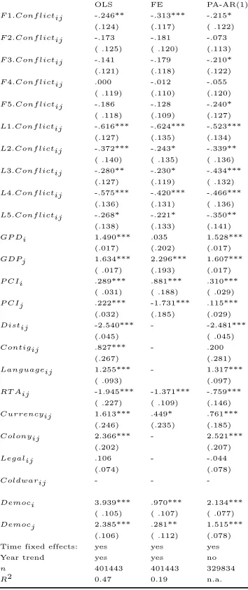
In using current conflict levels to explain current trade I introduce an endo-geneity bias because causality goes in both directions. Including past values is one possibility to overcome this problem. I also include leads or future outcomes of conflict to explain trade. This allows me to test Morrow’s hypothesis of ra-tional expectations which assumes that firms consider past outcomes of conflict before they decide to trade. Including leads completes the rational expectation model and was not done in this particular context before. I include ten leads and ten lags of conflict in my regressions. Table 2 summarizes the results. I report only results for five leads and lags to conserve space.

Most of the variables remain similar in sign and significance. Per capita income (PCI) changes the sign but remains significant in the fixed effect model. Including lags of conflict reveals that previous level of hostility have a long-lasting and negative effect on current trade. The history between two countries matters, such that tensions remain significant between two countries over time. In other words why should I trade with my enemy? Including leads of conflict shows in the pooled and fixed effect panel model, that the next period matters. If a firm expects a conflict next year, it will trade less today. The forward looking behavior can be explained by the profit maximization of firms where trade contracts are set in advance.

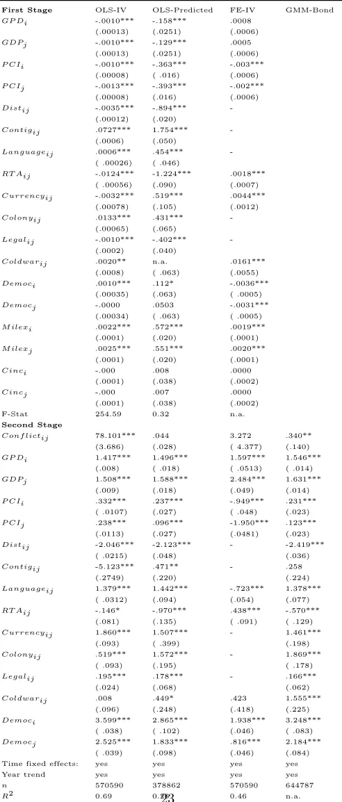
IV-model. I have two instruments available which explain conflict but likely not trade. I use military expenditures (M ilex) and a national military capability index (CIN C) both are available for most countries and come from the National Materials Capability dataset offered by the Correlates of War project (2010). It could be argued that parts of those instruments are linked with trade e.g. countries buy weapons which is part of trade. I will utilize a dynamic panel estimator suggested by Aranello and Bond (1991) which uses past values of the endogenous variable as its own instruments (GMM-Bond). It has the advantage that it corrects for autocorrelation and makes the choice of instruments easier. One drawback is that the GMM estimator looses some of its reliability in large T studies.

Table 3 shows results for the first stage regressions where available and the second stage. I find thatCIN C does not explain conflict, although it is com-monly used in the literature (Russet and Oneal 1999, Barbieri 2001). Instead military expenditures have a positive effect on conflict outcomes. The more a country spends on national defense, the more likely it is to show its power. Tests for exogeneity of the instruments in the IV-models (Hansen and Sargent), as well the GMM-Bond model, show that the first stage instruments are valid. The sign and significance of the regressors remains meaningful. Finally the first stage F-statistics are promising, where available. I will discuss the results for the first stage regressor, when I focus on the adverse effects of trade on conflict. My main finding is that current conflict has a positive effect on current trade, but only remains significant in the OLS-IV and GMM-Bond model. Does it mean that conflict actually increases trade flows? It depends, but given that trade contracts have to be fulfilled, the occurrence of a conflict today does not affect current trade flows negatively. Another explanation could be that weapons are for many countries an important part of trade, for instance Germany set another record in 2011 in exporting military equipment and weapons3

. Given that many countries export and import military equipment, a positive effect is not unlikely at all. Furthermore after the end of the Cold War, not only the number of civil wars increased (Upsalla Database 2011), but also the number of MIDs. Barbieri and Schneider (1999) find that trade even takes place between enemies if the conflict or war is short.

3

5

Does trade affect conflict?

Trade can affect conflict negatively, positively or not at all. According to Po-lacheks (1980) welfare maximization model governments realize that gains of trade will be reduced by international conflict. The liberal peace hypothesis (Barbierie 1996) states that trade forces countries to communicate with each other. Communication leads to cooperation and finally peace. Trade therefore reduces international conflict. In the realist view of the world (Barbieri 1996) trade creates dependencies. When trade benefits are distributed assymetrically between two countries tensions may arise. Gowa (1994) shows that trade can create security externalities because gains of trade can be used for national de-fense. Trade has a positive effect on conflict. Finally Morrow (1999) argues that current trade has no effect on conflict because firms trade. Firms use in-formation on past conflict outcomes to decide to trade with another country or not.

I employ a gravity equation including GDP, per capita income (PCI) and two measurements of distance (Distij and Contigij). Distance can be ambiginous

in explaining conflict. Conflicts can be between neighboring countries for in-stance over territory e.g. India and Pakistan but also between countries farther away from each other. Especially after the end of the Cold War, UN and Nato missions were conducted in countries like Somalia, the former Yugoslavia or the Iraq. Conflicts in the past were between colonies and colonizers e.g. between former African colonies and their European motherlands in the 1960’s. I use official language spoken and colonial ties to account for historical ties. The legal background matters, because countries which have a similar system fight less (Martin, Mayer and Thoenig 2008). Democracies are known to be more peace-ful, which is known as the democratic peace hypothesis. I include the Unified Democracy Score (UDS) to measure the level of democracy, because UDS offers more observations than the standard Polity IV variable. Military expenditures have an effect on international conflict. Countries which spend more on their military are more likely to display and use force. I include a variable indicating if two countries are in a formal military alliance defined as a defense treaty4

. To account for time effects common to every trade dyad, I include a variable indicating the Cold War period, time fixed effects and a year trend.5

4

Declared as a type 1 alliance according to the COW definition.

5

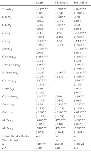
Because of the binary nature of the conflict variable MID, I use non-linear estimation methods.6

Table 4 summarizes the results for the pooled logit (col-umn 1), the fixed effect logit model (col(col-umn 2) and a population average GEE logit estimator (column 3).7

The GEE estimator is standard in political science for this particular question.

In the pooled logit model (Table 4) current trade has a negative and highly significant impact on current conflict, which is in favor of the liberal peace hy-pothesis. GDP does not explain conflict outcomes. In a model without military expenditure GDP has a positive effect on conflict.8

After including military ex-penditures, GDP becomes insignificant. Military expenditures are part of GDP and explain the variation in conflict outcomes significantly. Countries spend-ing more on national defense are more likely do display and use their military power. Wealthier countries, in terms of higher per capita income (PCI), are less involved in international conflict. Distance measured as actual distance between two capitals has a negative impact on conflict, while neighboring countries are more likely to be involved in a conflict. Sharing a common official language and having a history as a colony and colonizer increases the potential for con-flict between two countries. Many countries having an interstate concon-flict also share a common language for example China and Taiwan or Korea and South Korea. The legal background has no significant impact on conflict, similarly for alliances. Finally democracy, measured by the Unified Democracy Score, has a strong negative impact on conflict, as predicted by the democratic peace hypothesis.

The fixed effect logit model is different from the underlying pooled logit model. Changes in conflict outcomes are explained. If a dyad was in conflict at timetbut not at t−1 it enters the model. If a dyad has the same outcome in

two consecutive periods it does not enter the model. Time invariant variables drop out, because they do not contain new information.

Column 2 of table 4 shows the results for the fixed effect logit model. Trade has a highly significant and negative impact on changes in conflict levels. GDP

fixed effects.

6

I used linear probability models for pooled version but do not report results here. The LPM and pooled logit results do not differ substantially. Results can be requested from the author.

7

I do not show results for a random effects logit estimator, but the results are similar in sign and significance compared to the underlying pooled logit estimator.

8

has a negative effect. Countries larger in economic size fight less. Per capita income (PCI) has no explanatory power. Policy variables like democracy and military expenditures have a similar impact as in the pooled logit model. Al-liance is significant in the fixed effect model and reduces conflict.

The population average logit model is similar in sign and significance as the pooled logit model. Slightly different results are caused by the AR(1) link, while the GEE model without an assumed link within groups would converge to the pooled logit model. Trade has a negative impact on conflict.

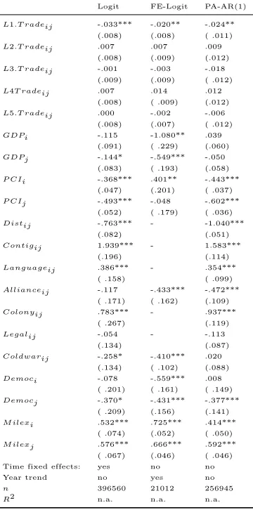
In using current trade to explain current conflict levels I introduce a simul-taneity bias in my models. I include 10 lags of trade and present the results table 5. Furthermore I can answer the question if the trade history between countries matters in reducing interstate conflict or not. I report only five lags of trade to conserve space.

Only previous period’s trade levels explain current conflict in the same em-pirical models as above (table 5). Governments act short-sighted when an in-terstate conflict occurs and do not account for past trade relationships. Head et Al find (2010) that former colonies, after breaking off from their motherlands, start trading again with each other a few years later. Given that movements for independence initiated decolonization, the conflict is forgotten a few years later. Other control variables remain similar in sign and significance in all three models.

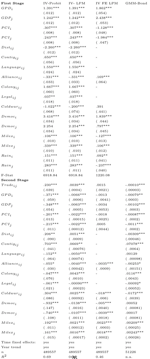
Another strategy to deal with endogeneity, caused by using current trade levels to explain current conflict, is to use an instrumental variable approach. The instrument to explain bilateral trade is rainfall. Rainfall matters for many countries in affecting economic outcomes for instance GDP growth (Miguel, Satyanath and Sergenti Ernest 2004). Trade is linked to GDP. I use annual rainfall data from the Tyndall Centre for Climate Change Research . Rainfall data are available from 1961 to 2000, which limits the sample. I employ an IV Probit model. To account for the panel nature I use an fixed effect IV linear probability panel model (IV FE LPM). It could be argued that rainfall is not the best instrument available. To account for possible limitations I use a dynamic panel GMM estimator, where past trade levels are instruments for the endogenous variable trade (GMM-Bond).

rainfall is added as an instrument. First stage results are valid in sign and significance of the regressors, as well the F-test values. Tests for exogeneity of the instruments (Hansen and Sargent) indicate that rainfall is indeed exogenous. Column 1 presents the results for the IV-probit model. Standard gravity variables like GDP, per capita income (PCI) and distance have the expected signs and are highly significant. Alliances have a negative effect on trade and behave as regional trade agreement in the trade conflict models.9

Military ex-penditures have a positive effect on trade. Many countries import the military equipment they need. Rainfall has a strong positive impact on current trade. In the second stage trade has a positive effect on conflict, which could be explained by increased tensions through trade dependencies. Most variables are similar in sign and significance as before. The negative impact of GDP is more signif-icant. Military expenditures and democracy have the same impact on conflict. The actual distance between two countries has a positive impact. While many conflicts during the Cold War were between neighboring countries, after 1992 conflicts were between countries further away, for instance the involvement of NATO allies in Iraq or in the former Yugoslavia.

The fixed effect panel model (column 2) performs similar to the IV-probit model in the first stage.10

After accounting for endogeneity and changes over time, the second stage shows different results. Current trade has no significant effect on conflict. Standard gravity variables loose their significance, while policy variables like military expenditures and democracies remain significant.

The GMM Bond model (column 3) differs, because past values of the en-dogenous variables are used as instruments. Trade has a negative impact on conflict. Variables like GDP, PCI and distance measures remain significant and similar in their signs. The democracy variables do not explain conflict outcomes but military expenditures do. Military expenditures have a strong and positive effect on conflict. Tests for exogeneity show that the instruments are valid.

9

Mansfield and Gowa (1997) show that regional trade agreements and alliance have the same effect on trade. It could be argued that regional trade agreements follow alliances.

10

6

Robustness checks

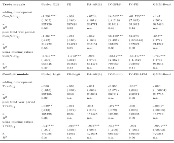
I perform three robustness checks. First I want to know how the level of devel-opment of a country affects the relationship between trade and conflict in my models. Second researchers argue that the democratic peace hypothesis is an artifact of the Cold War (Barbieri 1996). I limit the sample to the post Cold War period. Third I deal differently with missing values in assuming them to be zero. The results are summarized in table 7. To conserve space, I only report coefficients on the conflict and trade variable respectively. The first part of ta-ble 7 shows the results for the trade models. The second part of tata-ble 7 shows the results for the conflict models.11

I limit my analysis to current variables, because past outcomes did not change in the new setups.

The level of development is a known predictor for trade but also for con-flict. More developed countries are likely to trade more and are less involved in conflicts compared to less developed countries. I use the Human Development Index (HDI) to proxy for development. The HDI is available from 1970 onwards and covers most countries. Other possible development indicators e.g. school enrollment, available in the World Development Indicator database, cover the same years. Nonetheless the HDI summarize most indicators available sepa-rately into one index. Countries in the sample are developed on the average (HDI=0.61). HDI has a positive and significant effect on trade in my models, and a negative or no effect on conflict.12

The effect of current conflict on current trade is mixed. Conflict looses some of the previous significance. Adding HDI to the conflict models shows that trade has no effect on conflict.

The post Cold War period covers the years 1992 to 2001. For the post Cold War period the results are mixed for both models. Conflict has a negative impact on trade in the pooled model but looses significance in the fixed effect panel model. I find a positive effect of conflict on trade in the instrumental variable models. The effect of trade on conflict is not significant or slightly negative for the post Cold War period. Trade has a positive effect on conflict only in the IV probit model.

The IMF trade statistic includes many missing values for trade relationships which are unlikely to have any significant amount of trade. Although it is re-ported as missing or not available, trade is likely to be zero. Why should Tuvalu

11

Results for other control variables can be requested from the author.

12

trade with the Oman? Israel does not trade with its neighboring countries for obvious political reasons, but trade is not coded as zero. I treat missing values as zero, which increases the sample by more than 200.000 observations. The ef-fect of conflict on trade is negative and significant, even in models which showed a different result before. Conflict reduces trade. I find similar results in the con-flict models. Trade reduces concon-flict in most setups, while I found mixed results before. The reciprocal relationship between trade and conflict persists but the question is, can we trust these results? Although it is common to declare miss-ing values in trade as zero, Head et Al (2010) argue that this can bias results, because we do not know for sure if missing trade observations are really zero or not.

7

Conclusion

The discussion if trade and interstate conflict are related has left a mixed picture in the literature. Trade and conflict can be negatively, positively or not related at all. The causality goes both ways. Trade can affect conflict (the liberal peace hypothesis), or conflict can affect trade (Morrows rational expectation hypothesis).

My research design adds to the discussion by changing the structure of the world to a rectangle, accounting for endogeneity and the panel structure in both setups. The underlying empirical model is a gravity equation. I cover the period 1948 to 2001, as well almost all countries of the world.

effect on trade. To account for possible limitations with my instrumental vari-ables, I employ a dynamic panel GMM estimator. The GMM estimator has the advantage to use past outcomes of the endogenous variable as instruments.

I treated missing trade values as real missing. My robustness checks deal differently with missing trade values in assuming them to be zero. The negative relationship between trade and conflict is stronger in this setup. Another set of robustness checks include a development indicator (HDI) and focuses on the post Cold War period only, the trade conflict relationship looses some of its significance.

A

References

[1] Anderton H. Charles and Carter R. John (2001) ”The Impact of War on Trade: An interrupted time-series study”, Journal of Peace Research, Vol. 38 No.4, pp.445-457

[2] Arellano M. and Bond S. (1991) ”Some tests of specification for panel data: Monte Carlo evidence and an application to employment equations”, The Review of Economic Studies, Vol. 58, pp.277297

[3] Barbieri Katherine (1996) ”Economic Interdependence: A path to peace or source of interstate conflict?”, Journal of Peace Research, Vol. 33 No.1, pp.29-49

[4] Barbieri Katherine and Levy Jack (1999) ”Sleeping with the Enemy: The Impact of War on Trade”, Journal of Peace Research, Vol. 36 No. 4, p.463-479

[5] Barbieri Katherine and Schneider Gerald (1999) ”Globalization and Peace: Assessing New Directions in the Study of Trade and Conflict”, Journal of Peace Research, Vol. 36 No.4, pp.387-404

[6] Barbieri Katherine and Levy Jack (2001) ”Does War Impede Trade? A Response to Anderton and Carter”, Journal of Peace Research, Vol.38 No.5, pp.619-624

[7] Barbieri Katherine (2003) ”The Liberal Illusion: Does trade promote peace?”, The University of Michigan Press

[8] Barbieri Katherine, Keshk Omar and Pollins Brian (2008) ”Correlates of War Project Trade Data Set Codebook, Version 2.0”,

http://correlatesofwar.orglast accessed 03/30/2011

[9] Bayoumi Tamim and Eichengreen Barry (1997) ”Is Regionalism simply a Diversion? Evidence from the Evolution of the EC and EFTA”, in NBER Regionalism vs. Multilateral Trade Agreements, p.141-168

[11] Copeland C. Dale (1996) ”Economic Interdependence and War - A theory of trade expectations”, International Security, Vol. 20 No. 4, pp.5-41

[12] Green P. Donald, Kim Soo Yeon and Yoon H. David (2001) ”Dirty Pool”, International Organization, Vol.55 No.2, pp.441-468

[13] Ghosn Faten, Glenn Palmer, and Stuart Bremer (2004) ”The MID Data Set, 19932001: Procedures, Coding Rules, and Description.”, Conflict Management and Peace Science, Vol. 21, pp.133-154

[14] Head Keith, Mayer Thierry and Ries John (2010) ”The erosion of colonial linkages after independence”, Journal of International Economics, Vol.81, p.1-14

[15] Keshk Omar, Pollins Brian M. and Reuveny Rafael (2004) ”Trade still follows the flag: The primacy of politics in a simultaneous model of in-terdependence and armed conflict”, The Journal of Politics, Vol.66 No.4, pp.1155-1179

[16] Hegre Havard, Oneal John R. and Russet Bruce (2009) ”Trade does pro-mote peace: New simultaneous estimates of the reciprocal effects of trade and conflict”, Working Paper Yale University

[17] Liang Kung-Yee and Zeger L. Scott (1986) ”Longitudinal data analysis using generalized linear models”, Biometrica, Vol.73 No.1, pp.13-22

[18] Li Quan and Sacko David (2002) ”The (Ir)Relevance of Militarized Dis-putes of International Trade”, International Studies Quarterly, Vol.46 No.1, pp.11-43

[19] Long Andrew G. (2008) ”Bilateral Trade in the Shadow of Armed Con-flict”, International Studies Quarterly, Vol. 52, pp.81-101

[20] Mansfield D. Edward and Gowa Joanne (1993) ”Power Politics and Inter-national Trade”, American Political Science Review, Vol.87 No.2, pp.408-420

[22] Martin Philippe, Mayer Thierry and Thoenig Matthias (2008) ”Make trade not war?”, Review of Economic Studies, Vol. 75 No.3, pp.865-900

[23] Miguel Edward, Satyanath Shanker and Sergenti Ernest (2004) ”Economic Shocks and Civil Conflict: An Instrumental Variables Approach”, The Journal of Political Economy, Vol.112 No.4, pp.725-753

[24] Morrow D. James, Siverson M. Randolph and Tabares E. Tressa (1998) ”The Political Determinants of International Trade: The Major Powers, 1907-1990”, American Political Science Review, Vol.92 No.3, pp.649-661

[25] Morrow D. James (1999) ”How Could Trade Affect Conflict?”, Journal of Peace Research, Vol.36 No.4, pp.481-489

[26] Mitchell, T.D., Carter, T.R., Jones, P.D., Hulme,M., New, M (2003) ”A comprehensive set of high-resolution grids of monthly climate for Europe and the globe: the observed record (1901-2000) and 16 scenarios (2001-2100)”’, Journal of Climate, submitted

[27] Oneal R. John and Ray James Lee (1997) ”New Tests of the Democratic Peace: Controlling for Economic Interdependence, 1950-85”, Political Re-search Quarterly, Vol. 50 No.4, pp.751-775

[28] Oneal R. John and Russet Bruce (1999) ”Assessing the Liberal Peace with Alternative Specifications: Trade Still Reduces Conflict”, Journal of Peace Research, Vol. 36 No.4, pp.423-442

[29] Oneal R. John and Russet Bruce (2001) ”Clear and Clean: The Fixed Effects of Liberal Peace”, International Organization, Vol.55 No.2, pp.469-485

[30] Oneal R. John (2003) ”Empirical Support for the liberal peace” in Mans-field Edward and Pollins Brian ”Economic Interdependence and Interna-tional Conflict”, pp.189-206

[31] Pemstein Daniel, Meserve Stephen and Meltan, James (2010) ”Democratic Compromise: A Latent Variable Analysis of Ten Measures of Regime Type”, Political Analysis, August 2010

[33] Polachek Solomon W. (1997) ”Why Democracies Cooperative more and fight less: The Relationship Between International Trade and Coopera-tion”, Review of International Economics, Vol. 5 No.3, pp.295-309

[34] Polachek Solomon W. (1999) ”Liberalism and Interdependence: Extend-ing the Trade-Conflict Model”, Journal of Peace Research, Vol.36 No.4, pp.405-422

[35] Polachek Solomon W. (2007) ”Trade, Peace and Democracy: An analy-sis of dyadic dispute” in Sandler Todd and Hartley Keith ”Handbook of Defense Economics”, Vol.2, Chapter 31

[36] Pollins Brian M. (1989a) ”Does Trade still follow the flag?”, American Political Science Review, Vol. 83 No.2, pp.465-480

[37] Pollins Brian M. (1989b) ”Conflict, Cooperation, and Commerce: The Effect of International Political Interactions on Bilateral Trade Flows”, American Journal of Political Science, Vol. 33 No.1, pp.737-61

[38] Reuveny Rafael (2000) ”The Trade and Conflict Debate: A survey of theory, evidence and future research”’, Peace Economics, Peace Science and Public Policy, Vol.6 No.1, pp.23-49

[39] Singer, J. David, Bremer Stuart and Stuckey John (1972) ”Capability Distribution, Uncertainty, and Major Power War, 1820-1965.” in Bruce Russett (ed) Peace, War, and Numbers, Beverly Hills, Sage, pp. 19-48

[40] Tinbergen, Jan (1962), Shaping the World Economy: Suggestions for an International Policy, The Twentieth Century Fund

[41] United Nations (2010) ”Human Development Report 2010: - The Real Wealth of Nations: Pathways to Human Development”, http://hdr. undp.org/en/reports/global/hdr2010/, last accessed 12/16/2011

B

Tables

OLS FE PA-AR(1)

Conf lictij -1.063** -1.338*** .145 (.446) (.359) (.181)

GP Di 1.551*** 1.397*** 1.561*** (.014) (.147) (.014)

GDPj 1.636*** 2.532*** 1.627***

(.014) (.141) (.014)

P CIi .223*** -.680*** .249*** (.023) ( .133) (.023)

P CIj .125*** -1.931*** .054** (.024) ( .131) (.023)

Distij -2.444*** - -2.37***

(.036) ( .037)

Contigij .417* - -.020

(.222) (.244)

Languageij 1.370*** - 1.431***

(.077) (.082)

RT Aij -.754*** -.768*** .067 (.142) ( .081) (.087)

Currencyij 1.582*** .398** .933*** (.212) (.201) (.161)

Colonyij 1.848*** - 1.711***

( .179) (.188)

Legalij .182*** - .160**

(.062) (.065)

Coldwarij .058 -.025 -1.338*** (.036) (.037) (.047)

Democi 3.436*** 1.813*** 2.020*** ( .088) (.099) (.070)

Democj 2.288*** .719*** 1.469*** ( .089) (.097) (.070) Time fixed effects: yes yes yes

Year trend yes yes no

n 644787 644787 507828

R2 0.48 0.26 n.a.

Table 1: Trade gravity equation - 1948 to 2001

OLS FE PA-AR(1)

F1.Conf lictij -.246** -.313*** -.215* (.124) (.117) ( .122)

F2_{.Conf lictij} -.173 -.181 -.073 ( .125) ( .120) (.113)

F3.Conf lictij -.141 -.179 -.210* (.121) (.118) (.122)

F4.Conf lictij .000 -.012 -.055 ( .119) (.110) (.120)

F5_{.Conf lictij} -.186 -.128 -.240* ( .118) (.109) (.127)

L1.Conf lictij -.616*** -.624*** -.523*** (.127) (.135) (.134)

L2.Conf lictij -.372*** -.243* -.339** ( .140) ( .135) ( .136)

L3.Conf lictij -.280** -.230* -.434*** (.127) (.119) ( .132)

L4.Conf lictij -.575*** -.420*** -.466*** (.136) (.131) ( .136)

L5.Conf lictij -.268* -.221* -.350** (.138) (.133) (.141)

GP Di 1.490*** .035 1.528*** (.017) (.202) (.017)

GDPj 1.634*** 2.296*** 1.607***

( .017) (.193) (.017)

P CIi .289*** .881*** .310*** ( .031) ( .188) ( .029)

P CIj .222*** -1.731*** .115*** (.032) (.185) (.029)

Distij -2.540*** - -2.481***

(.045) ( .045)

Contigij .827*** - .200

(.267) (.281)

Languageij 1.255*** - 1.317***

( .093) (.097)

RT Aij -1.945*** -1.371*** -.759*** ( .227) ( .109) (.146)

Currencyij 1.613*** .449* .761*** (.246) (.235) (.185)

Colonyij 2.366*** - 2.521***

(.202) (.207)

Legalij .106 - -.044

(.074) (.078)

Coldwarij - -

-Democi 3.939*** .970*** 2.134*** ( .105) ( .107) ( .077)

Democj 2.385*** .281** 1.515*** (.106) ( .112) (.078) Time fixed effects: yes yes yes

Year trend yes yes no

n 401443 401443 329834

R2 0.47 0.19 n.a.

Table 2: Trade gravity equation - 1948 to 2001 - Lag and Leads of Conflict

First Stage OLS-IV OLS-Predicted FE-IV GMM-Bond

GP Di -.0010*** -.158*** .0008 (.00013) (.0251) (.0006)

GDPj -.0010*** -.129*** .0005

(.00013) (.0251) (.0006)

P CIi -.0010*** -.363*** -.003*** (.00008) ( .016) (.0006)

P CIj -.0013*** -.393*** -.002*** (.00008) (.016) (.0006)

Distij -.0035*** -.894*** -(.00012) (.020)

Contigij .0727*** 1.754*** -(.0006) (.050)

Languageij .0006*** .454*** -( .00026) ( .046)

RT Aij -.0124*** -1.224*** .0018*** ( .00056) (.090) (.0007)

Currencyij -.0032*** .519*** .0044*** (.00078) (.105) (.0012)

Colonyij .0133*** .431*** -(.00065) (.065)

Legalij -.0010*** -.402*** -(.0002) (.040)

Coldwarij .0020** n.a. .0161*** (.0008) ( .063) (.0055)

Democi .0010*** .112* -.0036*** (.00035) (.063) ( .0005)

Democj -.0000 .0503 -.0031*** (.00034) ( .063) ( .0005)

M ilexi .0022*** .572*** .0019*** (.0001) (.020) (.0001)

M ilexj .0025*** .551*** .0020*** (.0001) (.020) (.0001)

Cinci -.000 .008 .0000 (.0001) (.038) (.0002)

Cincj -.000 .007 .0000 (.0001) (.038) (.0002)

F-Stat 254.59 0.32 n.a.

Second Stage

Conf lictij 78.101*** .044 3.272 .340** (3.686) (.028) ( 4.377) (.140)

GP Di 1.417*** 1.496*** 1.597*** 1.546*** (.008) ( .018) ( .0513) ( .014)

GDPj 1.508*** 1.588*** 2.484*** 1.631***

(.009) (.018) (.049) (.014)

P CIi .332*** .237*** -.949*** .231*** ( .0107) (.027) ( .048) (.023)

P CIj .238*** .096*** -1.950*** .123*** (.0113) (.027) (.0481) (.023)

Distij -2.046*** -2.123*** - -2.419***

( .0215) (.048) (.036)

Contigij -5.123*** .471** - .258

(.2749) (.220) (.224)

Languageij 1.379*** 1.442*** -.723*** 1.378*** ( .0312) (.094) (.054) (.077)

RT Aij -.146* -.970*** .438*** -.570***

(.081) (.135) ( .091) ( .129)

Currencyij 1.860*** 1.507*** - 1.461***

(.093) ( .399) (.198)

Colonyij .519*** 1.572*** - 1.869***

( .093) (.195) ( .178)

Legalij .195*** .178*** - .166***

(.024) (.068) (.062)

Coldwarij .008 .449* .423 1.555***

(.096) (.248) (.418) (.225)

Democi 3.599*** 2.865*** 1.938*** 3.248*** ( .038) ( .102) (.046) ( .083)

Democj 2.525*** 1.833*** .816*** 2.184***

( .039) (.098) (.046) (.084)

Time fixed effects: yes yes yes yes

Year trend yes yes yes yes

n 570590 378862 570590 644787

R2 0.69 0.26 0.46 n.a.

Table 3: Dealing with Endogeneity - 1948 to 2001 - IV regressions

*** significant at 1 %, ** significant at 5%, * significant at 10%. I use clustered standard errors. For the

Logit FE-Logit PA-AR(1)

T radeij -.017*** -.028*** -.022*** ( .006) (.004) ( .006)

GDPi -.065 -.366** .030

(.075) ( .155) (.055)

GDPj -.075 -.367** .003

(.070) ( .150) (.051)

P CIi -.341 -.175 -.448*** ( .043) (.146) ( .034)

P CIj -.463*** -.172 -.688*** ( .049) ( .144) ( .034)

Distij -.798*** - -1.042***

(.066) (.046)

Contigij 1.885*** - 1.484***

(.171) (.103)

Languageij .536*** - .376***

( .141) ( .090)

Allianceij -.304* -.276** -.274*** (.159) (.141) ( .099)

Colonyij .747*** - .920***

( .225) (.104)

Legalij -.140 - -.047

(.120) (.079)

Coldwarij .514*** -.300 .439*** ( .174) (.085) (.086)

Democi -.154 -.693*** .362*** (.175) ( .159) ( .139)

Democj -.368** -.610*** -.671*** ( .184) ( .158) (.134)

M ilexi .488*** .473*** .405*** ( .059) (.046) (.045)

M ilexj .538*** .474*** .559*** (.055) ( .044) ( .041) Time fixed effects: yes no no

Year trend no no no

n 549377 25090 300723

R2 0.30 0.26 n.a.

Table 4: Conflict gravity equation - 1948 to 2001

Logit FE-Logit PA-AR(1)

L1.T radeij -.033*** -.020** -.024** (.008) (.008) ( .011)

L2_{.T radeij} .007 .007 .009 (.008) (.009) (.012)

L3.T radeij -.001 -.003 -.018 (.009) (.009) ( .012)

L4T radeij .007 .014 .012 (.008) ( .009) (.012)

L5.T radeij .000 -.002 -.006 (.008) (.007) ( .012)

GDPi -.115 -1.080** .039

(.091) ( .229) (.060)

GDPj -.144* -.549*** -.050

(.083) ( .193) (.058)

P CIi -.368*** .401** -.443*** (.047) (.201) ( .037)

P CIj -.493*** -.048 -.602*** (.052) ( .179) ( .036)

Distij -.763*** - -1.040***

(.082) (.051)

Contigij 1.939*** - 1.583***

(.196) (.114)

Languageij .386*** - .354***

( .158) ( .099)

Allianceij -.117 -.433*** -.472*** ( .171) ( .162) (.109)

Colonyij .783*** - .937***

( .267) (.119)

Legalij -.054 - -.113

(.134) (.087)

Coldwarij -.258* -.410*** .020 (.134) ( .102) (.088)

Democi -.078 -.559*** .008 ( .201) ( .161) ( .149)

Democj -.370* -.431*** -.377*** ( .209) (.156) (.141)

M ilexi .532*** .725*** .414*** ( .074) (.052) ( .050)

M ilexj .576*** .666*** .592*** ( .067) (.046) ( .046) Time fixed effects: yes no no

Year trend no yes no

n 396560 21012 256945

R2 n.a. n.a. n.a.

Table 5: Conflict gravity equation - 1948 to 2001 - Lag of Trade

First Stage IV-Probit IV- LPM IV FE LPM GMM-Bond

GP Di 1.391*** 1.391*** 1.862*** (.012) ( .012) (.054)

GDPj 1.242*** 1.242*** 2.438***

(.012) (.012) ( .053)

P CIi .307*** .307*** -1.128*** (.008) ( .008) (.048)

P CIj .243*** .243*** -1.984*** (.008) (.008) ( .047)

Distij -2.260*** -2.260*** -( .012) (.012)

Contigij .650*** .650*** -(.056) ( .056)

Languageij 1.550*** 1.550*** -(.024) ( .024)

Allianceij -.331*** -.331*** .169*** (.033) (.033) (.064)

Colonyij 1.667*** 1.667*** -(.060) (.060)

Legalij .037** .037*** -(.018) (.018)

Coldwarij -1.022*** -.200*** .391 (.068) (.074) (.441)

Democi 3.416*** 3.416*** 1.839*** (.034) (.034) ( .044)

Democj 2.254 2.254*** .797*** (.034) (.034) ( .045)

M ilexi .106*** .106*** -.127*** ( .010) (.010) (.013)

M ilexj .339*** .339*** .106*** (.010) ( .010) (.012)

Raini .151*** .151*** .092** (.011) (.011) (.041)

Rainj .283*** .283*** -.237*** (.011) ( .011) (.040)

F-Stat 6918.84 6918.84 1220.08

Second Stage

T radeij .230*** .0039*** .0015 -.00010*** (.039) (.0004) (.0021) (.00003)

GP Di -.371*** -.0066*** -.0013 -.00079** ( .059) ( .0006) ( .0041) (.0003)

GDPj -.348*** -.0063*** -.0034 -.00102***

(.054) ( .0005) (.0053) ( .0003)

P CIi -.201*** -.0022*** -.0018 -.00087*** (.013) ( .00015) (.0025) ( .0002)

P CIj -.215*** -.0022*** .0005 -.0011*** ( .011) (.00012) (.0044) ( .0002)

Distij .206** .0051*** - -.00309***

( .090) ( .0009) (.00046)

Contigij .703*** .0669** - .07078***

( .041) ( .00076) ( .0064)

Languageij -.152** -.0050*** - .00129

( .064) (.00074) ( .00098)

Allianceij -.055* -.0040*** -.0035*** -.00253* ( .030) (.00042) ( .0009) ( .00151)

Colonyij -.047*** .0043*** - .0116***

(.076) ( .0010) (.0043)

Legalij -.061*** -.00090*** - -.00092*

(.021) ( .00023) (.00052)

Coldwarij .304*** .0025*** -.018*** -.0172*** (.086) (.00092) ( .006) ( .0039)

Democi -.932*** -.0138*** -.005*** .00052 (.147) ( .0016) (.0040) ( .00081)

Democj -.740*** -.0107*** -.0039*** .00017 ( .108) ( .0011) (.0018) ( .00081)

M ilexi .192*** .0021*** .0023*** .00209*** ( .011) (.00012) ( .0003) (.00025)

M ilexj .161*** .0016*** .0018*** .00243*** ( .015) ( .00017) (.0002) (.00026)

Time fixed effects: yes yes yes yes

Year trend yes yes yes yes

n 489557 489557 489557 51226

R2 0.69 0.26 0.46 n.a.

Table 6: Dealing with Endogeneity - 1960 to 2000 - IV regressions

*** significant at 1 %, ** significant at 5%, * significant at 10%. I use clustered standard errors. For the

Trade models Pooled OLS FE PA-AR(1) IV-2SLS IV-FE GMM-Bond

adding development

Conf lictij -1.232*** -.009 -.0701 14.502*** -61.725*** -.147 ( .302) (.140) (.101) ( 4.519) (7.842) (.200)

n 327426 327426 294774 311612 311612 327426

R2 0.50 0.32 n.a. 0.48 0.16 n.a. post Cold war period

Conf lictij -1.360*** -.263 -.062 58.159*** 84.673 .653** (.422) (.180) (.160) (9.498) (163.044) (.272)

n 214222 214222 208184 187022 187022 214222

R2 0.53 0.35 n.a. 0.30 0.00 n.a. using missing values

Conf lictij -3.613*** -1.773*** -.006 -33.57*** -55.377*** -.739*** ( .390) (.231) (.079) (2.262) ( 4.182) (.173)

n 953646 953646 864476 793050 793050 953646

R2 0.47 0.33 n.a. 0.41 0.11 n.a.

Conflict models Pooled Logit FE-Logit PA-AR(1) IV-Probit IV-FE-LPM GMM-Bond

adding development

T radeij -.006 -.000 -.011 -6.386 .001* -.000

( .010) (.009) (.009) (5.074) (.004) ( .00004)

n 297785 9568 203881 260912 260912 297785

R2 0.29 n.a. n.a. n.a. 0.00 n.a. post Cold War period

T radeij -.029** -.001 .003 .472*** .000 -.0001*

(.013) (.019) (.013) (.079) (.003) (.00005)

n 165798 2024 151428 126303 126303 165799

R2 0.33 n.a. n.a. n.a. 0.00 n.a. using missing values

T radeij -.027*** -.039*** -.013*** .613*** -.001 -.0001*** ( .005) (.003) (.003) ( .100) ( .001) (.00003)

n 773085 34854 425608 666530 666530 720263

R2 0.31 n.a. n.a. n.a. 0.00 n.a.

Table 7: Robustness Checks