Mathematical Analysis and Simulation of an Age Structured Model of Two Patch for Tuberculosis (TB)

(1)

http://www.scirp.org/journal/am

ISSN Online: 2152-7393 ISSN Print: 2152-7385

Mathematical Analysis and Simulation

of an Age-Structured Model

of Two-Patch for

Tuberculosis (TB)

Badjo Kimba Abdoul Wahid, Saley Bisso

Department of Mathematics and Computer Science, Abdou Moumouni University, Niamey, Niger

Abstract

This paper studied a structured model by age of tuberculosis. A population divided into two parts was considered for the study. Each subpopulation is submitted to a program of vaccination. It was allowed the migration of vaccinated people only be-tween the two patches. After the determination of ℜ

( )

ψ

_and ℜ₀_{, the local and}

global stability of the disease-free equilibrium was studied. It showed the existence of three endemic equilibrium points. The theoretical results were illustrated by a nu-meric simulation.

Keywords

Age-Structured, Reproductive Number, Two-Patch, TB, Stability, Simulation

1. Introduction

Tuberculosis (TB) (short for tubercle bacillus) is a widespread, infectious disease caused by various strains of mycobacteria, usually Mycobacterium tuberculosis (MTB). Tu-berculosis typically attacks the lungs, but can also affect other parts of the body [1]. To be infected bacilli must penetrate deep into the alveoli, but the contagiousness of the disease is relatively low and depends on the immune system of subjects. Individuals at highest risk are young children, adults, deficient elderly, and people living in preca-rious socio-economic conditions, in nursing or whose immunity is deficient (AIDS, immunosuppressive therapy ...) [2]. This is one of the most common old infectious diseases [3][4], with about two billion people being currently infected. There are

How to cite this paper: Wahid, B.K.A. and Bisso, S. (2016) Mathematical Analysis and Simulation of an Age-Structured Model of Two-Patch for Tuberculosis (TB). Ap-plied Mathematics, 7, 1882-1902.

http://dx.doi.org/10.4236/am.2016.715155 Received: August 8, 2016

Accepted: September 27, 2016 Published: September 30, 2016

http://creativecommons.org/licenses/by/4.0/

(2)

about nine million new cases of infection each year and two million deaths per year according to WHO estimations [3][5]. For more information, many authors have worked on the epidemiology of tuberculosis [1]-[3] [5]-[13]. In many developing countries in general and sub-Saharan Africa particularly, TB is the leading cause of death, accounting for about two million deaths and a quarter of avoidable adult deaths

[11].

It is well known that factors such as the emergence of drug resistance against tu-berculosis, the growth of the incidence of HIV in recent years, as well as other dis-eases favor the development of Koch bacillus in the body call for improved strategies to control this deadly disease [2] [10] [14]. Last May, the World Health Assembly approved an ambitious strategy for 20 years (2016-2035) to put an end to World TB epidemic (World Day of fight against tuberculosis—March 24, 2015). In literature, several articles discussed about coinfection: TB-HIV/AIDS and the most recent is [2]. Nowadays, it is not a secret for everyone that fighting against infectious diseases is also a fight against poverty. Humans are traditionally organized into well-defined so-cial units, such as families, tribes, villages, cities, countries or regions are good exam-ples of patches [11] [12]. For this study, two subpopulations were considered and each was subjected to a vaccination program. However, only the vaccinated individu-als can migrate from one patch to another. Despite that we have neglected the relapse rate, to avoid any risk of treated individuals’ reactivation, any migration between patches was allowed. After proving that the problem is well defined and it has a unique solution if the initial condition is given, we are able to calculate the reproduction of numbers ℜ

( )

ψ

_and ℜ₀_{. We have established the existence conditions for three}

en-demic equilibrium points, and the conditions of local and global stability of the equi-librium point without disease. Finally, numerical simulations illustrate clinical out-comes. This paper is organized as follows: Section 2 introduces the two-patch model structured in age to study the dynamics of TB transmission. The existence of positive and unique solutions is demonstrated in Section 3. The point of equilibrium without disease, reproductive numbers ℜ

( )

ψ

_and ℜ₀_{are defined in the section 4 with the}

local and global stability of the disease-free equilibrium point. The existence of three endemic equilibrium points is proven in Section 5. Some numerical simulation re-sults are given in Section 6. In Section 7, we have a discussion, conclusion and further work.

2. Parameters and Mathematical Model Formulation

Two-patch age structured model of tuberculosis was considered. The model is to split the population into two subpopulations. The recruitment is only possible in the class of susceptible and the vaccinated individuals were able to migrate between the two sub-populations. Each subpopulation is divided into five classes based on their epidemio-logical status: susceptible, vaccinated, latent, infectious or treated. We denote these subgroups S t a_i

( )

, , v t a_i

( )

, , L t a_i

( )

, , I t a_i

( )

, and J t a_i

( )

, respectively. The birth

(3)

disease relative to the patch i and the rate of natural mortality. The time and age de-pended of the force of infection of the subpopulation i is

λ

_i

( )

t a, and vaccination rate

is

ψ

i

( )

a ; p a ai

(

, ′

)

is the probability that an infective individual of age a′ will have

contact with and successfully infect a susceptible individual of age a, c ai

( )

is the

age-specic per-capita contact/activity rate (all of these functions are assumed to be con-tinuous and to be zero beyond some maximum age). A fraction φi of newly infected

individuals of the sub-population i is assumed to undergo a fast progression directly to the infectious class Ii. Rates of migration, of susceptible passage to latent infectious

state and treatment are respectively ρi; ki and ri. Risk reduction rates of treatment

and vaccination are σi and δi respectively, 0≤

σ

i≤ −

(

1

φ

i

)

, 0≤ ≤ −

δ

i

(

1

φ

i

)

, in this

paper i=1, 2.

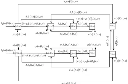
The age-structured model for the transmission of TB (see Figure 1) is described by the following system of partial differential equations:

( )

( ) ( )

( )

( ) ( )

( )

( ) (

) ( )

( )

(

( )

)

( )

(

( )

)

( )

( ) ( )

( )

1 1 1 1 1

1 1 1 1 1 1 1 1 1 1

1 1 1 1 1 1 1 1 1

1 1 1 1 1

, , , ,

, , 1 , , , ,

, , , , ,

, , ,

S t a b a N t a t a a a S t a

t a

L t a t a S t a J t a V t a k a L t a

t a

I t a k L t a r a a I t a t a S t a

t a

J t a r I t a t a

t a

λ ψ µ

λ φ σ δ µ

µ µ φ λ

σ λ

∂ ∂

 ₊  ₌ ₋_ ₊ ₊ _

_∂ _∂   

 

∂ ∂

 ₊  ₌ _ ₋ ₊ ₊ _₋ ₊

_∂ _∂   

 

∂ ∂

 ₊  ₌ ₋ ₊ ₊ ₊

_∂ _∂ 

 

∂ ∂

 ₊  ₌ ₋

_∂ _∂ 

 

(

( )

)

( )

( ) ( )

( )

(

( )

)

( )

( ) ( )

( )

( ) (

) ( )

( )

(

( )

)

( )

1

1 1 1 2 2 1 1 1 1

2 2 2 2 2

2 2 2 2 2 2 2 2 2 2

2 2 2

,

, , , , ,

, , , ,

, , 1 , , , ,

, ,

a J t a

V t a a S t a V t a a t a V t a

t a

S t a b a N t a t a a a S t a

t a

L t a t a S t a J t a V t a k a L t a

t a

I t a k L t a

t a

µ

ψ ρ ρ µ δ λ

λ ψ µ

λ φ σ δ µ

+

∂ ∂

 ₊  ₌ ₊ ₋ ₊ ₊

_∂ _∂ 

 

∂ ∂

 ₊  ₌ ₋_ ₊ ₊ _

_∂ _∂   

 

∂ ∂

 ₊  ₌ _ ₋ ₊ ₊ _₋ ₊

_∂ _∂   

 

∂ ∂

 ₊  ₌

_∂ _∂ 

 

(

( )

)

( )

( ) ( )

( )

(

( )

)

( )

( ) ( )

( )

(

( )

)

( )

2 2 2 2 2 2

2 2 2 1 1 2 2 2 2

, , ,

, ( , ) , ,

, , , , ,

r a a I t a t a S t a

J t a r I t a t a a J t a

t a

V t a a S t a V t a a t a V t a

t a

µ µ φ λ

σ λ µ

ψ ρ ρ µ δ λ

                    

 − + + +



 ∂ ∂ ₊  ₌ ₋ ₊

__∂ _∂ _ 

 ∂ ₊ ∂  ₌ ₊ ₋ ₊ ₊

_∂ _∂ 

 



(1)

with initial and boundary conditions:

( )

( ) ( )

( )

( ) ( )

( )

( ) ( )

( )

2 1

0 0 0

0 0

, 0 , d

, 0 , 0 , 0 , 0 0

0, ; 0, ; 0,

0, ; 0,

a

i _a i

i i i i

i i i i i i

i i i i

S t b a N t a a

L t V t I t J t

S a S a L a L a V a V a

I a I a J a J a

 ₌



 = = = =



 = = =



= =



∫

and

( )

,

( ) ( )

₀

( )

_{( ) (}

, ,

)

d ,

a _i

i i i i

I t a

t a a c a p a a a

N t a

λ β + ′ _′ _′

=

′

∫

, assume that assume that

(

_,

)

( ) ( )

ˆ

i i i

(4)

[image:4.595.124.557.71.354.2]

Figure 1. Flow chart of the two-patch model for tuberculosis disease transmission.

(see Greenhalgh, 1988 [15] and Dietz Schenzle, 1985 [16]), and

( )

1 1 1 1 1

2 2 2 2 2

, , , , , ,

, , , , ,

N t a S t a L t a I t a J t a V t a

S t a L t a I t a J t a V t a

= + + + +

+ + + + + .

By summing equations of system (1) and (2), we obtain the following equations for the total population N t a

( )

, :

( )

(

( )

)

( )

( ) ( )

( )

2

( ) ( )

1

1 1 2 2

, , , ,

, 0 a , d

a

N t a b a a N t a a I t a a I t a

t a

N t b a N t a a

µ µ µ

 ∂ ₊ ∂  ₌ ₋ ₋ ₋

 

 ∂ ∂  

 ₌



∫

(3)

where b a

( )

=b a1

( )

+b a2

( )

; a1 and a2 are respectively the minimum and maximum

age of procreation and a+ is the maximum age of an individual, with a+ < +∞. Let

( )

_{( ) ( )}

( )

_{( )}

( )

_{( )}

( )

_{( ) ( )}

( )

_{( )}

, ,

, ; ,

, ,

,

, ,

, ; , .

, ,

i i

S t a L t a

s t a l t a

N t a N t a

I t a i t a

N t a

J t a V t a

j t a v t a

N t a N t a



= =

 

 ₌

  

 ₌ ₌



(4)

(5)

( )

( ) ( )

( ) ( ) ( )

( )

( ) (

) ( )

( )

(

( )

( ) ( )

)

( )

(

( ) ( )

)

( )

1 1 1 1 1 1 2 2 1

1 1 1 1 1 1 1 1 1 1 1 2 2 1

1 1 1 1 1 2 2 1 1

, , , , ,

, , 1 , , , , , ,

, , , ,

s t a b a t a a b a a i t a a i t a s t a

t a

l t a t a s t a j t a v t a k b a a i t a a i t a l t a

t a

i t a r a b a a i t a a i t a i t a

t a

λ ψ µ µ

λ φ σ δ µ µ

µ µ µ φ λ

∂ ∂

 ₊  ₌ ₋_ ₊ ₊ ₋ ₋ _

_∂ _∂   

 

∂ ∂

 ₊  ₌ _ ₋ ₊ ₊ _₋ ₊ ₋ ₋

_∂ _∂   

 

∂ ∂

 ₊  _{= −} ₊ ₊ ₋ ₋ ₊

_∂ _∂ 

 

( ) ( )

( )

(

( ) ( )

)

( )

(

( )

( ) ( )

)

( )

( ) ( )

( )

( ) ( )

( )

1 1 1 1

1 1 1 1 1 1 1 2 2 1

1 1 1 1 1 1 2 2 1 1 1 2 2

2 2 2 2 1 1 2 2

, , ,

, , , , , ,

, , , , , , ,

, , ,

t a s t a k l t a

j t a r i t a t a b a a i t a a i t a j t a

t a

v t a b a t a a i t a a i t a v t a a s t a v t a

t a

s t a b a t a a b a a i t a a i

t a

σ λ µ µ

ρ δ λ µ µ ψ ρ

λ ψ µ µ

+

∂ ∂

 ₊  ₌ ₋ ₊ ₋ ₋

_∂ _∂ 

 

∂ ∂

 ₊  _{= −} ₊ ₊ ₋ ₋ ₊ ₊

_∂ _∂ 

 

∂ ∂

 ₊  ₌ ₋ ₊ ₊ ₋ ₋

_∂ _∂ 

 

( ) ( )

( )

( ) (

) ( )

( )

(

( )

( ) ( )

)

( )

(

( ) ( )

)

( )

( ) ( )

( )

2

2 2 2 2 2 2 2 2 2 1 1 2 2 2

2 2 2 1 1 2 2 2 2 2 2 2 2

2 2 2 2 2

, ,

, , 1 , , , , , ,

, , , , , , ,

, , ,

t a s t a

l t a t a s t a j t a v t a k b a a i t a a i t a l t a

t a

i t a r a b a a i t a a i t a i t a t a s t a k l t a

t a

j t a r i t a t

t a

λ φ σ δ µ µ

µ µ µ φ λ

σ λ

 

 

∂ ∂

 ₊  ₌ _ ₋ ₊ ₊ _₋ ₊ ₋ ₋

_∂ _∂   

 

∂ ∂

 ₊  _{= −} ₊ ₊ ₋ ₋ ₊ ₊

_∂ _∂ 

 

∂ ∂

 ₊  ₌ ₋

_∂ _∂ 

 

(

( ) ( )

)

( )

(

( )

( ) ( )

)

( )

( ) ( )

( )

1 1 2 2 2

2 2 2 2 1 1 2 2 2 2 2 1 1

, , ,

, , , , , , ,

a b a a i t a a i t a j t a

v t a b a t a a i t a a i t a v t a a s t a v t a

t a

µ µ

ρ δ λ µ µ ψ ρ

                         

+ − −

 

 ∂ ₊ ∂  _{= −} ₊ ₊ ₋ ₋ ₊ ₊

__∂ _∂ _ 

(5)

with boundary conditions

( )

, 0 ;

( ) ( ) ( )

, 0 , 0 , 0

( )

, 0 0

i i i i i i

s t = Λ v t =l t =i t = j t =

with Λ + Λ =1 2 1. The problem is well-posedness, the methode of proof is the same

used in [8].

3. Existence of Positive Solutions

In this section we will prove that the system (5) has a unique positive solution, and to achieve this we will write the system (5) in compact form (abstract Cauchy problem).

Consider the Banach space X defined by

(

1

(

)

10

0, ,

X = L a+ endowed with the

norm

2 5

1 1

ij i j

ϕ

= =

=

∑∑

₍₆₎

where

( )

(

( )

)

T 11 , 12 , 13 , 14 , 15 , 21 , 22 , 23 , 24 , 25

a a a a a a a a a a a X

ϕ = ϕ ϕ ϕ ϕ ϕ ϕ ϕ ϕ ϕ ϕ ∈

and . is the norm of 1

(

)

0,

L a+ . Let

(

)

{

s l i1, , ,1 1 j v s l i1, 1, 2, , ,2 2 j v2, 2 X+\ 0 s1 l1 i1 j v1, 1 s2 l2 i2 j2 v2 1

}

Ω = ∈ ≤ + + + + + + + + ≤ (7)

The state space of system (5), where

(

1

(

)

10

0,

X+= L+ a+ , and L1+

(

0,a+

)

denotes the

positive cone of 1

(

)

0,

L a+ . Let A be a linear operator defined by

( )( ) (

)

T

11, 12, 13, 14, 15, 21, 22, 23, 24, 25

Aϕ a = A A A A A A A A A A .

(8)

(6)

are not multiplied by si, li, ii, ji or vi in system (5) (see [17]), we obtain:

( )

(

( ) ( )

)

( )

( ) ( ) ( )

( )

(

( )

)

( )

( ) ( )

( )

( ) ( ) ( )

( )

(

( )

)

( )

1 1 1 1 1 1 1

1 1 1 1 1

1 1 1 1 1 1 2 2

2 2 2 2

2 2 , , , , , , , , , , , , , , , , , , , ,

i t a i t a r a b a i t a k l t a

t a

j t a j t a r i t a b a j t a

t a

v t a v t a b a v t a a s t a v t a

t a

s t a s t a a b a s t a

t a

a

l t a l t a k b a l t a

t a

i t a i

t a

µ

ρ ψ ρ

ψ ∂ ∂ = − − + + + ∂ ∂ ∂ ∂ = − + − ∂ ∂ ∂ _{= −} ∂ ₋ ₊ ₊ ₊ ∂ ∂ ∂ ∂ = − −_ + _ ∂ ∂ ∂ _{= −} ∂ ₋ ₊ ∂ ∂ ∂ ∂ = − ∂ ∂

( )

(

( ) ( )

)

( )

( ) ( ) ( )

( )

(

( )

)

( )

( ) ( )

( )

2 2 2 2

2 2 2 2 2

2 2 2 2 2 2 1 1

, , ,

, , , ,

, , , , , .

i

t a r a b a i t a k l t a

j t a j t a r i t a b a j t a

t a

v t a v t a b a v t a a s t a v t a

t a

µ

ρ ψ ρ

                − + + +   ∂ ∂ = − + −  ∂ ∂   ∂ _{= −} ∂ ₋ ₊ ₊ ₊  ∂ ∂ 

After replacing s1, l1, i1, j1, v1, s2, l2, i2, j2 and v2 by ϕ11

( )

a , ϕ12

( )

a ,

( )

13 a

ϕ _, ϕ₁₄

( )

a , ϕ15

( )

a ,ϕ21

( )

a , ϕ22

( )

a , ϕ23

( )

a , ϕ24

( )

a , ϕ25

( )

a in the system

(a) respectively, the coordinates of Aij are obtained from straight expressions (note

that each

( ) ( ) ( ) ( ) ( ) ( ) ( ) ( ) ( ) ( )

(

11 , 12 , 13 , 14 , 15 , 21 , 22 , 23 , 24 , 25

)

ij

A = f ϕ f ϕ f ϕ f ϕ f ϕ f ϕ f ϕ f ϕ f ϕ f ϕ

with respect to

ϕ

ij are given by:

( )

(

)

( ) ( )

(

)

( )

(

( )

)

12 12 1 12

13 1 12 13 1 1 13

14 1 13 14 14

15 1 11 15 1 15 2 25

21

d

0, , 0, 0, 0, 0, 0, 0, 0, 0

d d

0, , , 0, 0, 0, 0, 0, 0, 0

d d

0, 0, , , 0, 0, 0, 0, 0, 0

d d

, 0, 0, 0, , 0, 0, 0, 0,

d

0,

A b a k

a

A k r a b a

a

A r b a

a

A a b a

a

A

ϕ ϕ

ϕ ϕ µ ϕ

ϕ ϕ ϕ

ψ ϕ ϕ ρ ϕ ρ ϕ

  =_ − − + _     =_ − − + + _     =_ − − _     =_ − − + _   =

(

( ) ( )

)

( )

(

)

( ) ( )

(

)

( )

21 2 21

22 22 2 22

23 2 22 23 2 2 23

24 2 23 24 24

25 1 15 2

d

0, 0, 0, 0, , 0, 0, 0, 0

d d

0, 0, 0, 0, 0, 0, , 0, 0, 0

d d

0, 0, 0, 0, 0, 0, , , 0, 0

d d

0, 0, 0, 0, 0, 0, 0, , , 0

d

0, 0, 0, 0, ,

a b a

a

A b a k

a

A k r a b a

a

A r b a

a

A

ϕ ψ ϕ

ϕ ϕ

ϕ ϕ µ ϕ

ϕ ϕ ϕ

ρ ϕ ψ

 ₋ ₋ ₊        =_ − − + _     =_ − − + + _     =_ − − _  

=

( )

21 25

(

2

( )

)

25

d , 0, 0, 0,

d

a b a

a

ϕ ϕ ρ ϕ

                         _ _ − − +  _ _ 

. (9)

With

( )

(

( )

)

T

( )

11 , 12 , 13 , 14 , 15 , 21 , 22 , 23 , 24 , 25

a a a a a a a a a a a D A

(7)

where D A

( )

is the domain given by:

( )

{

[

) ( ) (

)

T

}

1 2

\ ij 0, , 0 , 0, 0, 0, 0, 0, , 0, 0, 0, 0 .

D A = ϕ∈X ϕ ∈AC a+ ϕ = Λ Λ

And AC

[

0,a+

)

denotes the set of absolutely continuous functions on

[

0,a+

)

. We also define a nonlinear operator F:X →X by:

( )( )

( ) (

(

)( )

)

(

( )

)

(

)( )

(

)

(

)

(

( )

)

(

)( )

(

)

(

( )

)

( )

(

)

(

)( )

)

( )

(

)

(

)( )

)

(

)( )

(

)

(

( )

)

(

)( )

(

)

(

)

1 1 13 11 1 13 2 23 11

1 13 1 11 1 14 1 15 1 13 2 23 12

1 1 13 11 1 13 2 23 13

1 13 2 23 1 1 13 14

1 13 2 23 1 1 13 15

2 2 23 21 1 13 2 23 21

2 23 2 21

1

( )

1

b a Q a a a

Q a a a

a a Q a

F a

b a Q a a a

Q a

ϕ

µ

ϕ

µ

ϕ ϕ

ϕ

ϕ ϕ

σ ϕ

δ ϕ

µ

ϕ

µ

ϕ ϕ

ϕ

µ

ϕ

µ

ϕ ϕ

µ

ϕ

µ

ϕ

δ

ϕ

µ

ϕ

µ

ϕ

σ

ϕ

µ

ϕ

µ

ϕ ϕ

ϕ

ϕ ϕ

− + +

− + + + +

+ +

+ −

=

− + +

− +

(

)

(

( )

)

(

)( )

(

)

(

( )

)

( )

(

)

(

)( )

)

( )

(

)

(

)( )

)

2 24 2 25 1 13 2 23 22

2 2 23 21 1 13 2 23 23

1 13 2 23 2 2 23 24

1 13 2 23 2 2 23 25

a a

Q a a a

a a Q a

σ ϕ

δ ϕ

µ

ϕ

µ

ϕ ϕ

ϕ

µ

ϕ

µ

ϕ ϕ

µ

ϕ

µ

ϕ

δ

ϕ

µ

ϕ

µ

ϕ

σ

ϕ

 

 

+ + +

 

 ₊ ₊ 

 

 ₊ ₋ 

 

 ₊ ₋ 

 

(10)

where Qi is a bounded linear operator on

(

)

1 0,

L a+ given by

(

)( )

( ) ( ) ( )

₀a ˆ

( ) ( )

_d

i i i i i

Q f a =c a

β

a g a

∫

+

β

a′ f a′ a′. (11) Let

( )

(

1

( ) ( ) ( ) ( ) ( ) ( ) ( ) ( )

., ,1 ., ,1 ., , 1 ., , 1 ., , 2 ., , 2 ., ,2 ., , 2

( ) ( )

., , 2 .,

)

u t = s t l t i t j t v t s t l t i t j t v t

thus, we can rewrite the system (5) as an abstract Cauchy problem:

( )

(

( )

)

( )

0

d d 0

u t Au t F u t

t

u u

 ₌ ₊

 

 ₌



(12)

where

( )

(

( ) ( ) ( )

( )

( ) ( ) ( )

( )

)

T

0 01 , 01 ,01 , 01 , 01 , 02 ,02 ,02 , 02 , 02 .

u a = s a l a i a j a v a s a l a i a j a v a

According to these results we have the following results (see [17]-[19]): Lemma 1. The operator F is continuously Fréchet differentiable on X.

Lemma 2. The operator A generates a C0-semigroup of the bounded linear opera-tors etA and the space Ω is positively invariant by etA.

Theorem 1. For each u0∈X+ there are a maximal interval of existence

[

0,tmax

)

and a unique continuous mild solution u t u

(

, 0

)

∈X+, t∈

[

0,tmax

)

for (12) such that

( )

₍

_{( )}

₎

0e ₀e d

t A t tA

u t =u +

∫

−ξ F u

ξ

Proof. The proof of this theorem can be found in [18]-[20]. 

4. The Disease-Free Steady State

4.1. Determination of the Disease-Free Equilibrium

(8)

sys-tem (5) must satisfy the following time-independent syssys-tem of ordinary differential eq-uations:

( )

( ) ( ) ( )

( ) ( )

( ) ( ) ( )

( )

( ) ( ) ( )

(

) ( )

( )

( ) ( )

(

)

( )

( ) ( ) ( )

( )

( ) ( )

( ) ( ) ( )

( )

( ) ( ) ( )

1 1 1 1 1 1 1 1 1 2 2 1

1 1 1 1 1 1 1 1 1 1 1

1 1 1 2 2 1

1 1 1 1 1 1 1 1 1 1 1 1 1 2 2 1

1 1 1 1 1 1 1 1

d d

d

1 d

d d

s a b a a c a g a a b a a i a a i a s a

a

l a a c a g a s a v a j a

a

b a k a i a a i a l a

i a k l a a c a g a s a r b a a a i a a i a i a

a

j a r i a a c a g a

a

β ψ µ µ

β φ δ σ

µ µ

φ β µ µ µ

σ β

= −_ Γ + + − − _

= Γ _ − + + _

− + − −

= + Γ −_ + + − − _

= −

(

Γ

( )

( ) ( )

)

( )

( ) ( )

( )

(

( ) ( ) ( )

( )

( ) ( )

)

( )

( ) ( ) ( )

( ) ( )

( ) ( ) ( )

( )

( ) ( ) ( )

(

) ( )

( )

( ) ( )

(

)

( )

1 1 2 2 1

1 1 1 2 2 1 1 1 1 1 1 1 2 2 1 1

2 2 2 2 2 2 2 1 1 2 2 2

2 2 2 2 2 2 2 2 2 2 2

2 1 1 2 2 2

2 2

d d

d

1 d

d d

b a a i a a i a j a

v a a s a v a a c a g a b a a i a a i a v a

a

s a b a a c a g a a b a a i a a i a s a

a

l a a c a g a s a v a j a

a

b a k a i a a i a l a

i a k l

a

µ µ

ψ ρ δ β µ µ ρ

β ψ µ µ

β φ δ σ

µ µ

+ − −

= + − Γ + − − +

= −_ Γ + + − − _

= Γ _ − + + _

− + − −

=

( )

( ) ( ) ( )

( )

( ) ( )

( ) ( ) ( )

( )

(

( ) ( ) ( )

( )

( ) ( )

)

( )

( ) ( )

( )

(

( ) ( ) ( )

( )

( ) ( )

)

( )

( ) ( )

2 2 2 2 2 2 2 2 2 1 1 2 2 2

2 2 2 2 2 2 2 2 1 1 2 2 2

2 2 2 1 1 2 2 2 2 2 1 1 2 2 2 2

0 d d

d d

ˆ _d

a

i i i

a a c a g a s a r b a a a i a a i a i a

j a r i a a c a g a b a a i a a i a j a

a

v a a s a v a a c a g a b a a i a a i a v a

a

a i a a

φ β µ µ µ

σ β µ µ

ψ ρ δ β µ µ ρ

β

+

                       

 ₊ _Γ ₋_ ₊ ₊ ₋ ₋ _

 

 

 ₌ ₋ _{Γ +} ₋ ₋

 

 = + − Γ + − − +

Γ =



∫

  

(13)

with initial value conditions

( )

0 ;

( )

0

( )

0

( )

0

( )

0 0.

i i i i i i

s = Λ l =i = j =v =

Therefore, we obtain the disease-free steady state

( )

(( ) ( )) ( ( ) ( ))

_{( )}

( )

( ) ( )

( )

0 d d

0

0 0 0 0 0

e e d

; 0

a a

i

i a b

b

i i i

i i i i i i

s a b

v a s a l a i a j a

η τ ψ τ τ

τ ψ τ τ

η η

− +

−∫ + ∫

 _{= Λ} ₊

 

 = Λ − = = =



∫

_.₍₁₄₎

4.2. Calculation of the Reproduction Numbers

ℜ

( )

ψ

-

ℜ

0

To study the stability of the disease-free steady state, we denote the perturbations of system by

( )

0

, ,

i i i

s t a s t a s a

l t a l t a l a

i t a i t a i a

j t a j t a j a

v t a v t a v a

 = +



= +

 

= +

 

= +



 ₌ ₊



(9)

The perturbations satisfy the following equations:

( )

( ) ( ) ( ) ( )

( ) ( )

( ) ( ) ( )

( )

(

)

( )

(

( )

)

( )

( ) ( ) ( ) ( ) (

) ( )

( )

( ) ( ) ( ) ( ) ( )

( ) ( )

(

)

( )

0

1 1 1 1 1 1 1 2 2 1

1 1

1 1 1

0 0

1 1 1 1 1 1 1 1

0

1 1 1 1 1 1 1 1 1

1 1 1

, , , , , , 1 , , ,

s t a t a c a g a a i t a a i t a s a

t a

b a a s t a

l t a b a k l t a

t a

t a c a g a s a v a

i t a k l t a a c a g a t s a

t a

r a b a i t a

t a

γ β µ µ

ψ

γ β φ δ

φ β γ

µ ∂ ∂  ₊  _{= −}_ ₋ ₋ _ _∂ _∂      − + ∂ ∂  ₊  _{= −} ₊ _∂ _∂      + _ − + _ ∂ ∂  ₊  ₌ ₊ _∂ _∂    − + + ∂ ∂  ₊ ∂ ∂

( )

( ) ( ) ( )

( )

( ) ( )

( )

(

( )

)

( )

( ) ( ) ( ) ( )

( ) ( )

(

)

( )

( ) ( ) ( ) ( )

( ) ( )

( ) ( ) ( )

( )

(

)

( )

1 1 1 1

1 1 1 2 2 1 1

0

1 1 1 1 1 1 2 2 1

0

2 2 2 2 2 1 1 2 2 2

2 2 2 , , , , , , , , , , , , , ,

j t a r i t a b a j t a

v t a a s t a v t a b a v t a

t a

a c a g a t a i t a a i t a v a

s t a t a c a g a a i t a a i t a s a

t a

b a a s t a

l t a b a

t a

ψ ρ ρ

δ β γ µ µ

γ β µ µ

ψ  ₌ ₋     ∂ ∂  ₊  ₌ ₊ ₋ ₊ _∂ _∂    − − − ∂ ∂  ₊  _{= −}_ ₋ ₋ _ _∂ _∂      − + ∂ ∂  ₊  _{= −} _∂ _∂   

(

)

( )

( ) ( ) ( ) ( ) (

) ( )

( )

( ) ( ) ( ) ( ) ( )

( ) ( )

(

)

( )

( ) ( ) ( )

( )

( ) ( )

( )

(

( )

)

( )

( ) ( ) ( ) ( )

( )

2 2 0 0

2 2 2 2 2 2 2 2

0

2 2 2 2 2 2 2 2 2

2 2 2

2 2 2 2

2 2 2 1 1 2 2

2 2 2 2 2 1

, 1 , , , , , , , , , ,

k l t a

t a c a g a s a v a

i t a k l t a a c a g a t s a

t a

r a b a i t a

j t a r i t a b a j t a

t a

v t a a s t a v t a b a v t a

t a

a c a g a t a i

γ β φ δ

φ β γ

µ

ψ ρ ρ

δ β γ µ

+   + _ − + _ ∂ ∂  ₊  ₌ ₊ _∂ _∂    − + + ∂ ∂  ₊  ₌ ₋ _∂ _∂    ∂ ∂  ₊  ₌ ₊ ₋ ₊ _∂ _∂    −

(

−

( )

( ) ( )

)

( )

( ) ( )

0

1 2 2 2

0

, ,

ˆ

( ) a , d

i i i

t a a i t a v a

t a i t a a

µ

γ +β

                                             −   =  

∫

(16)

with boundary conditions:

( )

, 0

( )

, 0

( )

, 0

( )

, 0

( )

, 0 0,

i i i i i

s t =l t =i t = j t =v t =

we consider the exponential solutions of system (16) of the form:

( )

, e ; , e

, e

, e ; , e

t t

i i i i

t

i i

t t

i i i i

s t a s a l t a l a

v t a v a

i t a i a j t a j a

λ λ λ λ λ  = =  ₌   ₌ ₌ 

.

(17)

(10)

( )

(

( )

)

( )

( ) ( ) ( )

( ) ( )

( ) ( ) ( )

( )

(

( )

)

( )

( ) ( ) ( ) (

) ( )

( )

( ) ( ) ( )

( )

(

( ) ( )

)

( )

(

( )

)

( )

(

( )

)

( )

( ) ( ) ( )

( )

0

1 1 1 1 1 1 1 1 1 2 2 1

0 0

1 1 1 1 1 1 1 1 1 1 1

1 1 1 1

1 1 1 1 1 1 1 1 1

d d

d

1 d

d d

s a b a a s a a c a g a a i a a i a s a

a

l a b a k l a a c a g a s a v a

a

i a a c a g a k l a r a b a i a

a

j a r i a b a j a

a

v a b a v a a c a g a a i

a

ψ λ β µ µ

λ β φ δ

φ β µ λ

λ

ρ λ δ β µ

 

= − + + − Γ_ − − _

 

= − + + + Γ _ − + _

= Γ + − + + +

= − +

= − + + −

(

Γ −

( )

( ) ( )

)

( )

( ) ( )

( )

(

( )

)

( )

( ) ( ) ( )

( ) ( )

( ) ( ) ( )

( )

(

( )

)

( )

( ) ( ) ( ) (

) ( )

( )

( ) ( ) ( )

( )

(

( ) ( )

)

( )

(

( )

)

( )

0

2 2 1 1 2 2

0

2 2 2 2 2 2 2 1 1 2 2 2

0 0

2 2 2 2 2 2 2 2 2 2 2

2 2 2 2

2 2

d d

d

1 d

d d

a a i a v a a s a v a

s a b a a s a a c a g a a i a a i a s a

a

l a b a k l a a c a g a s a v a

a

i a a c a g a k l a r a b a i a

a

j a r i a b a j a

a

v a b a

a

µ ψ ρ

ψ λ β µ µ

λ β φ δ

φ β µ λ

λ

ρ

− + +

 

= − + + − Γ_ − − _

 

= − + + + Γ _ − + _

= Γ + − + + +

= − +

= −

(

+

)

( )

(

( ) ( ) ( )

( ) ( )

)

( )

( ) ( )

( )

( ) ( )

0

2 2 2 2 2 1 1 2 2 2 2 2 1 1

0

ˆ _d

a

i i i

v a a c a g a a i a a i a v a a s a v a

a i a a

λ δ β µ µ ψ ρ

β

+

                         

 ₊ ₋ _Γ ₋ ₋ ₊ ₊

 

Γ =  

∫

(18)

with boundary conditions:

( ) ( ) ( )

0 0 0

( )

0

( )

0 0

i i i i i

s =l =i = j =v =

Let

( ) (

) ( )

0 0

( )

1

i i i i i

N_ψ a = −φ s a +δv a .

(19)

From Equation (18), we obtain:

( )

(( ) )d

( ) ( ) ( )

( )

0e d

a i

i a b k

i i i i i

l a = Γ

∫

−∫η τ+ +λ τ

β η

c

η

g

η

N_ψ

η η

(20)

( )

(( ) ( ))d

₍

_{( )}

_{( ) ( ) ( )}

₎

0e d

a

i i a b r a

i i i i i i i i

i a =

∫

−∫η τ+ + +λ µ τ k l

η

+ Γ

φ β η

c

η

g

η

. (21)

Hence, by Equations ((20) and (21)) after changing order of integration, we obtain:

( )

(( ) ( ) )d

_{( ) ( ) ( )}

0

_{( )}

( ( ) )d

0e e d d

a

i i i i i

i

a b r a r k

i i i i i i i i

i a c g s k N

η

η τ µ τ λ τ αµ τ τ

ψ _η

β η η η φ η η α η

−∫ + + +  −∫ + − 

= Γ _ + _

 

∫

. (22)

Injecting (22) in the expression of Γi, and dividing both sides the expression by Γi

(since Γ ≠_i 0), we get the characteristic equation:

( )

(( ) ( ) )d

_{( ) ( ) ( )}

0

_{( )}

( ( ) )d

0 0

ˆ

1 e e d d d

a

i i i i i

i

a a b r a r k

i a i ci gi i is k Ni a

η

ψ _η

β β η η η φ η η α η

+ −∫ + + +  −∫ + − 

= _ + _

 

∫

. (23)

Denote the right-hand side of Equation (23) by G

( )

λ i.e.:

( )

(( ) ( ) )d

( ) ( ) ( )

0

( )

( ( ) )d

0 0

ˆ _e a i i _e i i i _{d d}

i

a a b r a r k

i i i i i i i i

G a c g s k N d a

η

ψ _η

λ ₌ +β −∫ + + + β η η η φ η ₊ η −∫ + − α η

 

 

∫

. (24)

(11)

( )

(( ) ( ) )d

_{( ) ( ) ( )}

0

_{( )}

( ( ) )d

0 0

ˆ _e a i i _e i i i _d _{d d}

i

a a b r a r k

i

i i a i ci gi i is k Ni a

η

η τ µ τ τ αµ τ τ

ψ _η

ψ +β −∫ + + β η η η φ η η −∫ + − α η

ℜ = _ + _

 

∫

. (25)

We can obtain an expression for 0

i

ℜ _{in a similar way as the derivation of} ℜi

( )

ψ

by considering Equation (1) without vaccination; i.e., by assuming that ψi

( )

a ≡0 and

neglecting the equation of vaccinated. It can be shown that 0

( )

0

i i

ℜ = ℜ _{which is}

called the basic reproductive number (when a purely susceptible population is consi-dered) (see [8]).

( )

(( ) ( ) )d

( ) ( ) ( )

(

)

( ( ) )d

0 ₀ ˆ ₀e 1 e d d d

a

i i i i i

a a b r a r k

i

i i a i ci gi i ki i a

η

η τ µ τ τ αµ τ τ

η

β β η η η φ φ α η

+ −∫ + +  −∫ + − 

ℜ = Λ _ + − _

 

∫

(26)

Let

( )

max

( )

and 0 max 0.

i i

i

i i

ψ ψ

ℜ = ℜ ℜ = ℜ

4.3. Local Stability of the Disease-Free Equilibrium

Theorem 2. The infection-free steady-state (5) is locally asymptotically stable (l.a.s.) if

( )

ψ 1

ℜ < _{and unstable if} ℜ

( )

ψ >1. Proof. Noticing that

( )

0; lim

( )

0; lim

( )

.

i i i

G G G

λ λ

λ

→+∞ →−∞

′ < = = +∞

We know that Equation (23) has a unique negative real solution λ*_{if, and only if,}

( )

0 1

i

G < , hence, i

( )

1

i ψ

ℜ < (Also, Equation (23) has a unique positive (zero) real solution if ℜi

( )

ψi >1 (

( )

1

i i ψ

ℜ = _{). To show that}λ*_{is the dominant real part of}

roots of Gi

( )

λ , we let λ= +x iy be an arbitrary complex solution to Equation (23).

Note that

( )

(

)

( )

1=Gi λ = Gi x+iy ≤Gi x ,

indicating that

( )

*

e

R λ ≤λ . It follows that the infection-free steady state is l.a.s. if

( )

ψ 1

ℜ < _{, and unstable if} ℜ

( )

ψ >1. 

In this corollary, we have the three cases of the unstability of the disease free equili-brium.

Corollary 1. 1) whenever 1

( )

1 1

ψ

ℜ < _and 2

( )

2 1

ψ

ℜ > _,_{the disease free is locally}

asymptotically stable in the first patch and unstable in the second.

2) whenever 1

( )

1 1

ψ

ℜ > _and 2

( )

2 1

ψ

ℜ < _{, the disease free is unstable in the first}

patch and locally asymptotically stable in the second.

3) whenever 1

( )

1 1

ψ

ℜ > _and 2

( )

2 1

ψ

ℜ > _{, the disease free is unstable in the two}

patches.

4.4. Global Stability of the Disease-Free Equilibrium

Since µi

( )

a and i t ai

( )

, are bounded, there exists a positive constant Rc that satisfies

( ) (

)

2

1

0 a _i _i , d _c

i

i t a R

η µ τ τ τ τ

=

≤

_∫

∑

− + ≤

(*).

(12)

( ) ( ) ( )

₍

₎

₍

₎

₍

₎

(

) (

)

( ( )) ( ( ) ) ( ) ( ) ( )

₍

₎

( ( ) ) d d d d d

e , ( , ,

1 , e e d

e 1 e d .

a i i

a a

i i i i

a

i i i i i

r b

i i i i i i i

a

k b r k

i i

a

b r r k

i i i i

s t a k j t a v t a

s t a

k

η

η ξ

η

η ξ

µ τ τ τ

τ τ µ τ τ

η

τ µ τ τ µ τ τ

η

φ η η σ η η δ η η

φ η η ξ

φ φ ξ

− + + − + − − − + + − + − ∫ ∫ ∫ ∫ ∫  _{− +} ₊ _{− +} ₊ _{− +}   + − − +   

≤ Λ _ + − _

 

∫

Theorem 3. The disease-free equilibrium of system (5) is globally asymptotically sta-ble if ℜ <0 1 and

0 1 ln c

R <  _ ℜ  . Proof. The proof consist to show that

( )

, 0

i

i t a → ; j t ai

( )

, →0; l t ai

( )

, →0;

( )

0

( )

,

i i

s t a →s a and v t ai

( )

, → Λ −i si0

( )

a , when t→ +∞.

Integrating system (5) along characteristic lines we get

( )

(

( ) ( ) ( )

)

_{( ) ( ) ( ) (}

₎

(

)

(

) (

)

2

1 , d d

0

, e

, , 1 , d ,

a

i i i

i

a b i t a k

i i i i i

i i i i i i

l t a c g t a

j t a v t a s t a a t

η τ µ τ τ τ τ τ

_{β η}

_η

_{η λ}

_η

σ

η η δ

η

φ

η η

η

=

−∫ −∑ − + +

= − +

 

×_ − + + − + + − − + _ <

∫

₍₂₇₎

( )

(

( ) ( ) ( ) ( )

)

( ) ( ) ( ) (

)

(

)

2

1 , d

0

, e

, d ,

a

i i i i

i

a b i t a r

i

i i i i i i

i t a

c g t a k l t a a t

ξ τ µ τ τ τ µ τ τ

φ β ξ

ξ

ξ λ

ξ

ξ ξ

ξ

=

−∫ −∑ − + + +

=

×_ − + + − + _ <

∫

_.

₍₂₈₎

Injecting (27) in (28), and changing order of integration, we obtain:

( )

( ) ( )

( ) ( ) ( ) (

)

( ) ( )

( )

₍

₎

₍

₎

₍

₎

(

) (

)

( ( )) ( ( ) )

2

1 , d

0

d

d d

, e

e , , ,

1 , e e d d

a i i i a i i a

i i i i

a i t a

i i i i i

r b

i i i i i i i

a

k b r k

i i

i t a c g t a

s t a

η

η ξ

µ τ τ τ τ

µ τ τ τ

τ τ µ τ τ

η

β η η η λ η

φ η η ξ η

= − + − + + − + − + − ∑ ∫ ∫ ∫ ∫ = − +   ×_ − + + _ − + + − +     + − − + _ 

∫

. (29)

Injecting (29) in λi

( )

t , and changing order of integration, we obtain:

( )

( ) ( )

_{( ) ( ) ( ) (}

₎

( ) ( )

( )

₍

₎

₍

₎

₍

₎

(

) (

)

( ( )) ( ( ) )

2

1 , d

0 0

d

d d

ˆ _e

e , , ,

1 , e e d d d

a i i i a i i a

i i i i

a a i t a

i i i i i i

r b

i i i i i i i

a

k b r k

i i

t a c g t a

s t a a

η

η ξ

µ τ τ τ τ

µ τ τ τ

τ τ µ τ τ

η

λ β β η η η λ η

φ η η ξ η

+ = − + − + + − + − + − ∑ ∫ ∫ ∫ ∫ = − +   ×_ − + + _ − + + − +     + − − + _ 

∫

. (30)

By using corollary 2, inequality (*) and Fatou’s lemma, we have

( )

0

( )

lim eRc i lim sup .

i i

t→+∞λ t ≤ ℜ _t_→+∞ λ t

Since e c 0 1

Rℜ <i ,

( )

lim supt→+∞λi t 0

⇒ = ⇒

( )

0

( )

0

( )

lim , lim , lim , 0

lim , , lim , .

i t i i

t t

i i i i i

t t

i t a j t a l t a

s t a s a v t a s a

→+∞ →+∞ →+∞ →+∞ →+∞ = = =  

= = Λ −

 

(13)

1) the first sub-population if 1 0 1

ℜ < _and ₁

( ) (

₁

)

₁

0 1 0≤ _ηaµ τ i t− +a τ τ τ, d < ln_ℜ .

 

∫

2) the second sub-population if 2

0 1

ℜ < and 2

( ) (

2

)

2 0 1

0 a i t a , d ln .

ηµ τ τ τ τ

 

≤ − + _{< } 

ℜ  

∫

For this disease can disappear without any form of intervention, according to these results we must ensure that there is no new infected and the infectious rate does not reach a certain spread.

5. Existence of an Endemic State

There exists three endemic steady state of system (5) whenever ℜ

( )

ψ >1.

5.1. The First Boundary Endemic Equilibrium

Theorem 4. A boundary endemic equilibrium of the form

( )

(

)

* * * * * * * *

1 1 ,1 ,1 , 1 , 1 , 2 , 0, 0, 0, 2

E = s a l a i a j a v a s a v a whenever ℜ1

( )

ψ1 >1 and 2

( )

2 1

ψ

ℜ < _{. This means that the disease is endemic in the first sub-population}

and dies out in the second sub-population.

Proof. The method commonly used to find an endemic steady state for age-structure models consists of obtaining explicit expressions for a time independent solution of system (5)

( )

(

)

* * * * * * * *

1 1 ,1 ,1 , 1 , 1 , 2 , 0, 0, 0, 2

E = s a l a i a j a v a s a v a satisfies the following

equations:

( )

( ) ( ) ( )

( ) ( )

( ) ( ) ( )

( )

( ) ( ) ( )

(

) ( )

( )

(

( )

( ) ( )

)

( )

( ) ( ) ( )

( )

( ) ( )

( )

( ) ( ) ( )

1 1 1 1 1 1 1 1 1 1

1 1 1 1 1 1 1 1 1 1 1 1 1 1 1

1 1 1 1 1 1 1 1 1 1 1 1 1 1

1 1 1 1 1 1 1 1

d d

d

1 d

d d

d

s a b a a c a g a a b a a i a s a

a

l a a c a g a s a v a j a b a k a i a l a

a

i a k l a a c a g a s a r b a a a i a i a

a

j a r i a a c a g a

a

β ψ µ

β φ δ σ µ

φ β µ µ

σ β

∗ ∗ ∗ ∗

∗ ∗ ∗ ∗ ∗ ∗ ∗

∗ ∗ ∗ ∗ ∗ ∗

∗ ∗ ∗

 

= −_ Γ + + − _

 

= Γ _ − + + _− + −

 

= + Γ −_ + + − _

= −

(

Γ +

( )

( ) ( )

)

( )

( ) ( )

( )

(

( ) ( ) ( )

( )

( ) ( )

)

( )

( ) ( )

( ) ( ) ( )

( )

( ) ( )

( )

(

( )

( ) ( )

)

( )

( ) ( )

1 1 1

1 1 1 2 2 1 1 1 1 1 1 1 1

2 2 2 1 1 2

2 2 2 1 1 1 1 2

1 ₀ 1 1

d d

ˆ _d

a

b a a i a j a

v a a s a v a a c a g a b a a i a v a

a

s a b a a b a a i a s a

a

v a a s a v a b a a i a v a

a

a i a a

µ

ψ ρ δ β µ

ψ µ

ψ ρ µ

β

+

∗ ∗

∗ ∗ ∗ ∗ ∗ ∗

∗ ∗ ∗

∗ ∗ ∗ ∗ ∗

∗ ∗

        

 −

 

 ₌ ₊ ₋ _{Γ +} ₋

 

 ₌ ₋_ ₊ ₋ _

 

 

 ₌ ₊ ₋ ₋

 

Γ =



∫

(31)

with the initial conditions:

( )

* * * * *

1 1 1

0 ; 0 0 0 0 0.

i i i

s = Λ i =l =v = j =

Let

(

*

)

(

) ( )

* *

( )

*

( )

1 , 1 1 1 1 1 1 1 1

h η Γ = −φ s η +δv η +σ j η . (32)