Life cycle consumption: can single agent models get it right?

Munich Personal RePEc Archive

Life-cycle consumption: can single agent

models get it right?

Bick, Alexander and Choi, Sekyu

Goethe University Frankfurt, Universitat Autònoma de Barcelona

February 2011

Online at

https://mpra.ub.uni-muenchen.de/30910/

Life-Cycle Consumption:

Can Single Agent Models Get it Right?

Alexander Bick Goethe University Frankfurt

Sekyu Choi

Universitat Aut`onoma de Barcelona✯

May 2011

Abstract

In the quantitative macroeconomics literature, single agent models are widely used to explain “per-adult equivalent” data, which are obtained at the household level. In this paper we sug-gest a simple framework to understand the sources of bias when these models are used to make predictions for aggregate consumption. In both a theoretical and a quantitative exercise, we find that economies of scale in consumption inside the household are positively related to the bias introduced by the single agent approach in predicted consumption profiles over the life-cycle. We also do an external validation exercise, which suggests that economies of scale inside the household are rather large, pointing out the need to approach life-cycle consumption with models that consider households rather than single agents.

Keywords: Consumption, Life-Cycle Models, Households

JEL classification: D12, D91, E21, J10

✯_{email: [email protected] and [email protected]. We thank Jos´e-V´ıctor R´ıos-Rull, Dirk Krueger,}

Nicola Fuchs-Sch¨undeln, Josep Pijoan-Mas, Fabrizio Perri, Larry Jones, Nezih Guner, Juan Carlos Conesa, Tim

Ke-hoe, Greg Kaplan and seminar participants at Stockholm School of Economics, Universitat Aut`onoma de Barcelona

1

Introduction

To understand life-cycle consumption, single agent models are frequently used given their

tractability. In the quantitative macroeconomic literature, a standard approach entails

extract-ing per-adult equivalent consumption facts from household survey data and use them as targets to

be replicated by single agent models, which are also calibrated using per-adult equivalent

house-hold income. Some papers in this vein include Krueger and Perri (2006),Blundell, Pistaferri, and

Preston(2008), Kaplan and Violante(2009) and Guvenen and Smith(2010).1

However, this approach faces the inherent challenge that consumption decisions might depend

on household size and composition through non trivial channels. Cubeddu and R´ıos-Rull(2003) for

example, demonstrate that changes in marital status over the life-cycle affect aggregate savings in

the same order of magnitude as idiosyncratic income uncertainty. Although this approach has the

benefit of considering explicitly multi-person households, its drawback is that the model structure

becomes very complicated and computationally intensive to solve. The same criticism can be made

of models where demographic transitions occur endogenously, as in Aiyagari, Greenwood, and

Guner (2000) andMazzocco, Ruiz, and Yamaguchi (2007). In this paper, we abstract from these

difficulties and propose a simple framework in order to understand the sources and magnitudes of

bias when single agent models are used to make predictions for aggregate household consumption

or consumption related measures (i.e. welfare). Specifically, we are interested in predictions from

the standard incomplete markets model, which has become a workhorse in modern macroeconomic

analysis.

We follow Attanasio, Banks, Meghir, and Weber(1999) andGourinchas and Parker(2002) and

perform our analysis by extending the standard incomplete markets model to allow for

determin-istic changes in household size and composition during the life-cycle and let these changes affect

optimal decisions on consumption and savings in a unitary model approach. But unlike these two

papers, which use a general ’demographic’ taste shifter in the utility function, we propose a

formu-lation where economies of scales inside the household are considered explicitly through equivalence

1

Other papers present mixed empirical strategies. For example, Storesletten, Telmer, and Yaron (2004) use

household incomeper person from the PSID, while trying to match the cross-sectional variance in total household

consumption (without controlling for household size/composition). Another approach is inFern´andez-Villaverde and

scales.2 _{This setup accommodates both the case of single households (the Single model) and the}

case where household size varies during the life-cycle (what we label the Demographics model).

Although the Single model provides predictions for a single/bachelor consumption only and the

Demographics model predicts total household consumption, a common practice in the literature

is to transform household into individual consumption and vice versa through equivalence scales,

making predictions directly comparable.

Using a simple two period model of household consumption, we show theoretically that single

agent models introduce bias in predicted household consumption profiles: agents in these models

ignore the fact that the relative price of consumption across periods in which family size is changing

is affected by economies of scale inside the household.

We also perform a quantitative exercise and find that differences between household

consump-tion data from the Demographics and Single models can be substantial for mean consumption

profiles but not for inequality. The differences are increasing in the amount of economies of scale

present in the household. Intuitively, the bigger the economies of scale, the bigger the price

ef-fects in life-cycle consumption induced by changing household size which are ignored by theSingle

approach. If there are low economies of scale in consumption, a “household” would be just a

collec-tion of individuals sharing a physical address but nothing more: hence, modeling the economy as

if everyone lived in a single household would not entail significant loss of accuracy in predictions.

Finally, we compare our setup with the preference structure estimated in Attanasio, Banks,

Meghir, and Weber (1999) and infer the amount of economies of scale present in the household.

This external validation exercise suggests sizeable economies of scale, as prescribed byNelson(1993)

and similar to those found in Hong and R´ıos-Rull (2009). Following our argument, we conclude

that the study of life-cycle consumption should depart from the usage ofSinglemodels.

The structure of the paper is as follows: in Section 2 we discuss our proposed preferences for

the household and present theoretical predictions in a stylized two period framework. In Section

2

Equivalence scales are functions of household size and composition and typically used to deflate total household information (like consumption and income) by a number less than the actual household size. This approach has gained importance in the macro literature: in the 2010 special issue of the Review of Economic Dynamics, equivalence scales

are used to obtain consistent per-adult equivalent cross sectional facts for a wide range of countries (See Krueger,

Perri, Pistaferri, and Violante (2010) for a general description and Heathcote, Storesletten, and Violante (2010)

for the US economy). Another example isFern´andez-Villaverde and Krueger(2007), who discuss the properties of

3 we discuss the model we use to quantify these theoretical predictions. In Section4 we show the

quantitative features of the model and the calibration strategy while Section 7 shows our main

quantitative results. Section 2 presents our identification exercise, while in the last section, we

conclude.

2

Demographics in a Life-Cycle Model

In this section we investigate consumption in a two period model with a deterministic change in

household size. In particular, we assume that the household size is one in the first period (N₁ = 1),

e.g. a young person living alone, and larger than one in the second period (N2 >1), e.g. because

a child is born. The household receives an income stream y₁ and y₂, and can borrow up to the

natural borrowing constraint and save at an interest r which without loss of generality is set to

zero. Similarly, the discount factor is set to one, i.e. from the perspective of period one the utility

in period two is not discounted.

A standard approach in macroeconomics (obviously with more than two periods) is to assume

that households consist only of a single member, the bachelor household. Accordingly, such a

model cannot predict household consumption which is however the format for empirically observed

consumption data. Usually, this data is therefore divided by an equivalence scale which transforms

total household consumption into a per-adult equivalent consumption, against which the predictions

of the bachelor household are compared.

The three mechanisms through which household size affects the intra-temporal rate of

transfor-mation between expenditures and consumption services, and that are captured partially through

equivalence scales, are family/public goods, economies of scale, and complementarities. See for

example, Lazear and Michael(1980).

To ensure consistency between the model and the data, the income fed into the model is cleaned

for household size effects in a similar fashion by dividing household income with an equivalence

scale.3 Fern´andez-Villaverde and Krueger(2007) list a summary of representative equivalence scales

3

which are all normalized to one for single person households and are increasing in household size

by less than one. In our concrete setup this implies that the equivalence scaleφt equals one in the

first period and is larger than one in the second period, i.e. φ1 = 1 and φ2 > 1. We label this

approach as the Singlemodel and the corresponding optimization problem is thus

max

c1,S,c2,S

U =u(c_1,S) +u(c_2,S) (1)

subject to

c1,S +c2,S = y1 φ1

+ y2

φ2

≡YS. (2)

Not only do the consumption data come in household format but also the household consumption

choices are made taking into account household size. As a benchmark we therefore consider a model

in which household utility is affected by household sizeNt, which we label as Demographicsmodel,

and the optimization problem is represented by

max

c1,D,c2,D

U =u(c1,D, N1) +u(c2,D, N2) (3)

subject to

c1,D+c2,D=y1+y2≡YD. (4)

For the utility function we employ the following specification:

u(ct, Nt) =Ntu

ct φ(Nt)

. (5)

Household utility u(ct, Nt) is the product of the utility from per-adult equivalent consumption

u_φ(Nt)ct , and household size Nt, as the per-adult equivalent consumption is enjoyed by each

household member. While in the theoretical part of this paper, we will not rely on any specific

equivalence scale, our choice of the utility function can be best explained by considering a concrete

example, e.g. the widely used OECD equivalence scale which is given by

φOECD = 1 + 0.7(Nad−1) + 0.5Nch, (6)

Equation (6) it takes ✩ 1.7 of consumption expenditures to generate the same level of welfare out

of consumption for a two adult household that✩ 1 achieves for a single member household.

We think of this framework as the mildest departure from the Single model which considers

something akin to household size effects. The only additional twist in theDemographics model is

that household size and composition affect the (marginal) utility of consumption. As a consequence,

changes in household demographics over time impact the intertemporal allocation of consumption.

However, and as in the Single model, the optimal consumption saving choices are undertaken by

a single decision maker who equates marginal utilities over time. Note that the Single model

directly predicts an per-adult equivalent consumption because the household receives a per-adult

equivalent income. In the Demographics model, household consumption is predicted which then

has to be deflated by the equivalence scale in order to be comparable, i.e. c1,D

φ1 =

c1,D

1 and

c2,D

φ2 .

We are not the first to let demographics affect household utility. Attanasio, Banks, Meghir,

and Weber (1999) and Gourinchas and Parker (2002) introduce such an effect via a taste shifter

[exp(ξ1Nad +ξ2Nch)u(c)], while Fuchs-Sch¨undeln (2008) uses the same structure as in Equation

(5) but multiplies the utility from per-adult equivalent consumption by the equivalence scale φt

instead of household size Nt. Similarly, Cubeddu and R´ıos-Rull (2003), and Hong and R´ıos-Rull

(2007) use a different multiplication factor [min{Nad,2}] which accounts only for the “head” and

the spouse (if present) but not for dependents in the household. The latter three papers do not

provide any further justification for their choice of the multiplication factor. As outlined before,

the interpretation of an equivalence scale makes the total household size a more natural choice for

this multiplicative factor.

The following sections discuss how the Single model performs relative to our benchmark, the

Demographicsmodel.

2.1 Consumption Profiles

Result 1. _{The per-adult equivalent consumption profile in the Demographics model and Single}

model coincide if φ2 =N2.

This result can be immediately read of from the two Euler equations which for theDemographics

model is given by

u′(c1,D) = N2

φ2 u′

c2,D φ2

and for theSinglemodel by

u′(c1,S) =u′(c2,S). (8)

In both specifications only per-adult equivalent consumption appears. For theSinglemodel the

consumption levels c1,S and c2,S in fact reflect per-adult equivalent consumption because income

as an input to the optimization problem has already been deflated by the equivalence scale. For

theDemographicsmodel it is obvious in the second period as the household receives the (marginal)

utility from per-adult equivalent consumption c2,D

φ2 which is however also true in the first period

because household size is one in period one (φ1= 1).

Equation (8) predicts a flat per-adult equivalent consumption profile for theSinglemodel. The

per-adult equivalent consumption profile in theDemographicsmodel is however only flat ifN2 =φ2

but upward sloping ifN2> φ2, i.e. c1,D = c1_φ,D₁ < c2_φ,D₂ ,while the opposite is true forN2 < φ2. The

intuition behind this result can be best explained when decomposing the benefit of consuming one

additional unit of consumption in the second period in theDemographicsmodel which

1. is associated with the marginal utility of per-adult equivalent consumption in period one

h

u′c2,D

φ2

i

2. accrues to all household members reflected through the multiplication by household size [N2]

3. has to be divided by the equivalence scale [φ₂] because each household member does not get

the full unit to consume but only the fraction _φ1 2.

The larger household size in period two provides an incentive to allocate more consumption to

period two because the household enjoys a larger utility from consuming then because each unit of

per-adult equivalent consumption is enjoyed by more individuals (multiplication byN2). However,

in period two every unit of consumption has to be shared with more people which is reflected

through the division with the equivalence scale φ2. This in turn reduces the incentive to allocate

more consumption to period two. If φ2 =N2, the latter two effects cancel out and therefore

per-adult equivalent consumption in period one equals per-per-adult equivalent consumption in period two.

This case would however imply that the equivalence scale is larger than the household size and thus

no (or forφ2 > N2 even decreasing) economies of scale. This contradicts all empirically estimated

relevant caseφ2< N2 per-adult equivalent consumption in period two exceeds per-adult equivalent

consumption in period one. Relative to period one, the absolute loss in consumption in period two

because of the sharing across household members is outweighed by the fact that each household

member enjoys the extra per-adult equivalent consumption. Interestingly, such a configuration

provides an additional explanation for the hump observed in per-adult equivalent consumption

documented in Fern´andez-Villaverde and Krueger (2007). The ratio _φN₂ could be interpreted as a

change in the relative price of per-adult equivalent consumption induced by the change in household

size (relative to period one) which is ignored in the Singlemodel.

The Euler equation (7) gives of course also a clear prediction for the per-adult equivalent

consumption profile if the (marginal) utility is multiplied by a number smaller than actual household

size as assumed inCubeddu and R´ıos-Rull(2003),Hong and R´ıos-Rull(2007), andFuchs-Sch¨undeln

(2008). If the equivalence scale is smaller/equal/larger than the assumed multiplication factor,

per-adult equivalent consumption in theDemographicsmodel is upward sloping/flat/downward sloping.

2.2 Consumption Levels

Result 2. _{Life-time per-adult equivalent consumption in the Demographics model coincides with}

life-time per-adult equivalent consumption in the Singlemodel, if in theDemographicsmodel period

two household consumption c2,D and period two household income y2 coincide.

Life-time per-adult equivalent consumption from the Demographicsmodel can be written as

CD =c1,D+ c2,D

φ2

=y1+y2−c2,D

| {z }

c1,D

+c2,D

φ2

=y1+y2− φ2−1

φ2

c2,D (9)

while in the Single model life-time per-adult equivalent consumption equals life-time per-adult

equivalent incomeYS (see also Equation (2)):

CS =c1,s+c2,s =y1+ y2

φ₂ =YS (10)

theSinglemodel is given by

CD −CS=CD−YS = (y2−c2,D)

φ2−1 φ2

. (11)

which proofs Result 2. Whenever y2 > c2,D, i.e. the household in the Demographics model is a

borrower, the life-time per-adult equivalent consumption under the Demographics model is larger

than under the Single model. The opposite is true for y2 < c2,D, i.e. when the household in the

Demographicsmodel is a saver.

The intuition for this result can be explained best with a concrete example. Assume that the

household income is zero in the first period (y1 = 0), and positive in the second period (y2 >0).

In this case life-time per-adult equivalent income in the Single model is y2

φ2 which by the budget

constraint equals life-time per-adult equivalent consumption. In the Demographicsmodel in turn,

the household has the income y2 available for consumption. For any utility function satisfying

the Inada condition period one consumption will be positive such that c_2,D < y₂. Given that

household size is one in period one, in the calculation of life-time per-adult equivalent consumption

in theDemographicsmodel only period two consumption is deflated by the equivalence scale. Since

c2,D < y2, “less” in absolute terms is lost through the deflation by the equivalence scale in the

calculation of life-time per-adult equivalent consumption in the Demographicsmodel compared to

theSinglemodel.4

Essentially, Result 2 is the implication of a pure accounting exercise. The key driving force

behind is that households can shift consumption between periods whereas income is predetermined,

at least in any model with exogenous labor supply. If income and consumption allocations are not

fully synchronized, then transforming household income to a per-adult equivalent drives a wedge

between per-adult equivalent consumption in theDemographicsmodel and adult equivalent income,

and, as a direct consequence also, between per-adult equivalent consumption in theDemographics

and Singlemodel.

These differences in life-time per-adult equivalent consumption are also important in the

pres-ence of income heterogeneity. First, in the Single model the timing of income matters as it

de-termines life-time per-adult equivalent income. Even for the same life-time household income

4

More formally, fory1= 0 andy2 >0,c2,D< y2implies thatCD=y2−φ2_φ−1

2 c2,D> y2−

φ₂−1

φ₂ y2= y₂

yA

1 +y2A = y1B+y2B but a different timing

yA

1

yA

2

6

= yB1

yB

2

life-time per-adult equivalent incomes differ

in the Single but not in the Demographicsmodel. This implies an artificial inequality in life-time

per-adult equivalent consumption in the Single model that is not present in the Demographics

model. Second, it is straightforward to show that for heterogeneity in life-time household income

yA

1 +yA2 6=y1B+y2B but the same timing of income

yA

1

yA

2 = yB1

yB

2

, the implied inequality in life-time

per-adult equivalent consumption between the Single and Demographicsmodel is proportional to the

differences in life-time per-adult equivalent consumption in the two models, i.e. _Var(CVar(C_D)S) =CSA

CA

D

2

.

Note that the derivation and implications of Result 2 are completely independent of the

rela-tionship betweenN₂ andφ₂ which do however determinec_2,D and thus, for a given y₁ and y₂, the

relationship between the two per-adult equivalent consumption levels.

2.3 CRRA Preferences

In quantitative life-cycle models, CRRA preferences are the prevailing choice for the utility

func-tion. We now briefly discuss the role of the parameter of relative risk aversion in theDemographics

model. For our simple setup given by Equations (3) and (4) we obtain closed form solutions for

the optimal per-adult equivalent consumption allocation

c1,D =

1

1 +N2

φ2

1

α φ2

and c2,D

φ2 = N2 φ2 1 α

1 +N2

φ2

1

α φ2

. (12)

Since CRRA preferences are just a special case of the general utility function discussed before, we

can see here again that it is only the ratio N2

φ2 which determines the profile of the per-adult

equiv-alent consumption. Larger values of α imply a flatter profile, as the lower intertemporal elasticity

of substitution decreases the willingness to have differences in per-adult equivalent consumption

between the two periods.

As long as φ2 < N2 not only the per-adult equivalent but also the household consumption

profile is increasing. This is also true if we consider multiplication factors lower than the actual

household size for any value ofα >1.5

5

2.4 Summary

Two mechanisms introduce a bias into per-adult equivalent consumption predicted by theSingle

model relative to theDemographicsmodel. First, theSinglemodel ignores the change in the relative

price of per-adult equivalent consumption induced by changes in household size in the presence of

economies of scale. With CRRA preferences this channel looses importance as the coefficient

of relative risk aversion increases or equivalently as the intertemporal elasticity of substitution

decreases. Second, as an outcome of a pure accounting exercise, the Single model is generally

associated with a different life-time per-adult equivalent consumption than in the Demographics

model, which in the presence of income heterogeneity, feeds into inequality measures.

3

Quantitative Model

By constructing a quantitative model, our aim is to test and evaluate the implications of our

theoretical analysis with a simple, stripped-down version of a standard incomplete markets life-cycle

model, which can then be compared to actual US data.

Households start their economic life in period t₀ with zero assets. During their working life

until periodtw they receive a stochastic incomeytin every period. There is no labor supply choice.

From periodtw+ 1 onwards households are retired and have to live from their accumulated savings

during working life. We abstract from pensions. Life ends with certainty at ageT and households

do not leave bequests and cannot die with debt. Households have access to a risk-free bondawhich

pays the interest rate r. Households can borrow up to the natural borrowing constraint, i.e., an

age specific level of debt that they can repay for sure.

In the Demographics model household size changes over the life-cycle deterministically as in

Attanasio, Banks, Meghir, and Weber(1999) andGourinchas and Parker(2002) and is homogenous

across all households. The maximization problem is given by

also true for the per-adult equivalent consumption profile, is given by

α >1−lnδ2

lnφ2

where δ2 equals the multiplication factor which we have set equal to household size [δ2 =N2] whereas e.g.

max

{at+1}T_t=−_t1₀

E0 T

X

t=t0

βt−t0_N

tu

ct φt

subject to (13)

ct+at+1≤(1 +r)at+yt (14)

at+1≥amin,t. (15)

where φ is a function of household size and its composition (Nad,t and Nch,t). The income

process is given by:

lnyt=̺t+ǫt, (16)

where̺t is an age-dependent, exogenous experience profile and

ǫt=ρǫt−1+εt withεt∼N(0, σ2). (17)

The Euler equation to this problem is given by

Nt φt u′ ct φt

=β(1 +r)Nt+1

φt+1 Et u′ ct+1 φt+1 . (18)

The structure of the Single problem is very similar. Demographics do not affect the utility

function while incomeyt is deflated by household size through equivalence scalesφt:

max

{at+1}Tt=−t10

E0 T

X

t=t0

βt−t0_u(c

t) subject to (19)

ct+at+1≤(1 +r)at+ yt φt

(20)

at+1≥amin,t, (21)

withyt following the same process as described in Equations (16) and (17).

The Euler equation to this problem is given by

u′(ct) =β(1 +r)Et

4

Quantitative Features of the Model

A model period is one year. Agents start life at age 25, retire when 65 and live with certainty

until age 75. To maintain simplicity, agents receive no social security income when retired and

interest rates are zero (r = 0). We set the CRRA coefficient α to 1.57, the same value used in

Attanasio, Banks, Meghir, and Weber(1999). We then calibrateβsuch that household consumption

is the same at age 25 and at age 75. By doing this, we allow each model to better accommodate

the timing in the ’hump’ of household consumption seen in US data (see next section). In practical

terms, the range of calibrated β’s across models is centered with very low dispersion around 0.98,

a reasonable value for an annual model.

As for equivalence scales, we perform the analysis using both the OECD and the Nelson(1993)

scales. The OECD scale has the lowest economies of scale while the opposite is true for the Nelson

scale in a wide range of scales used in the literature. Each additional adult and child represent

(resp.) 0.7 and 0.5 adult equivalents according to the OECD; for the Nelson case the numbers are

0.06, 0.1 and 0.07 for each additional adult, the first child and each subsequent children respectively.

For example, a family of four (two adults and two children) is equivalent to 2.7 adults living alone

according to the OECD scale; the number for the Nelson scale is 1.23. For explicit formulations of

different equivalence scales used in the empirical consumption literature, see Table 1 inFern´

andez-Villaverde and Krueger (2007).

4.1 Income

We use data from the Current Population Survey, from 1984 to 2003. We use the March

supplements for years 1985 to 2004, given that questions about income are retrospective. We use

total wage income (deflated by CPI-U, leaving amounts in 2000 US dollars), and apply the tax

formula of Gouveia and Strauss(1994) to get after-tax income.6

We construct total household income Wiτ for household i observed in year τ, as the sum of

individual incomes in the household for all households with at least one full time/full year worker.

The latter is defined as someone who worked more than 40 hours per week and more than 40 weeks

per year and earned more than ✩2 per hour. Then, we estimate the following regression:

6

Table 1: Calibrated Parameters

ρ σ σ0

0.9906 0.0189 0.1575

log

_W

iτ φiτ

=D_iτage̺age+Xiτγ+ǫiτ (23)

where φiτ is an equivalence scale, D_iτage represents a set of age dummies of the head of household,

̺age and γ are estimated coefficients and εare estimation errors. Note that for the Demographics

model we use household income for the estimation, i.e. φiτ = 1 ∀ i, τ. We also control for cohort

effects and time effects by introducing birth year and year dummies inXiτ. 7

From this estimation, we are interested in the regression coefficients associated with age

dum-mies of the household head (experience profiles in the model). In our exercise below, we use

smoothed profiles, which we show in Figure1 for different choices of equivalence scales.

From the estimation residuals, we calibrate the income process in (17). Our calibration

pro-cedure is standard and follows Storesletten, Telmer, and Yaron (2004): we pick values of ρ and σ

in order to minimize the square difference between the profile of observed cross-sectional variances

of income and the simulated one (given the chosen parameters). We also pick values of σ₀, the

standard deviation for the unconditional distribution of the first income shockε0 in order to match

the cross sectional variance of income for our first age group (25 years old). We present these values

in Table 1. We discretize this calibrated process using the Rouwenhorst method, using 20 points

for the shock space. This methodology is specially suited for our case, given the high persistence

of the process, see the discussion in Kopecky and Suen(2010).

To maintain full comparability with our simple theoretical model, we perform anex-post

equiv-alization procedure for the income process in theSinglemodel: we use the same calibrated income

7_{Since year dummies are perfectly collinear with age and birth cohort dummies, we followFern´andez-Villaverde}

and Krueger(2007) and Aguiar and Hurst(2009) and include normalized year dummies instead, such that for each

yearτ

X

τ

γτ = 0 and

X

τ

τ γτ = 0

where{γτ}are the coefficients associated to these normalized year dummies. This procedure was initially proposed

Figure 1: Experience Profile for Households

10

10.2

10.4

10.6

10.8

Log annual income

20 30 40 50 60 70

age

Total OECD

Nelson

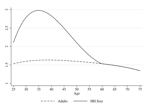
Figure 2: Profiles for Household Size and Composition

1

1.5

2

2.5

3

25 30 35 40 45 50 55 60 65 70 75 Age

Adults HH Size

profiles and shocks in both the Demographics and Single models (the calibration in Figure 1 and

Table 1) and then feed the per-adult equivalent experience profiles to the Single model. Besides

making the quantitative model more comparable to the theoretical model, this approach maintains

the same shock structure across considered equivalence scales, making the comparison of biases

more direct, since no extra ’noise’ is being introduced by different volatility parameters. This

would be the case for an alternative approach, or an ex-ante equivalization: estimating Equation

(23) with a particular equivalence scaleφiτ, resulting in different age profiles and calibrated income

shocks for the Singlemodel. Since the income has already been turned into per-adult equivalents

ex-ante, there is no need to do so in budget constraint (20).8

4.2 Family Structure

We use the March supplements of the CPS for years 1984 to 2003.9 _{For each household, we}

count the number of adults (individuals age 17+) and the number of children: individuals age 16

or less who are identified as being the “child” of an adult in the household. We restrict our sample

to consider households with at most 2 adults and 4 children. We compute two separate profiles:

one for number of adults and one for number of children. As above, we run dummy regressions to

extract life-cycle profiles, where the considered age is that of the head (irrespective of gender) and

control for cohort and year effects. After extracting these life-cycle profiles, we smooth them using

a cubic polynomial in age, and restrict the number of children to zero after age 60. The results of

this procedure are in Figure 2.

As inAttanasio, Banks, Meghir, and Weber(1999) andGourinchas and Parker(2002), the

num-ber for adults and children in the household over the life-cycle are not integers. The transformation

into adult equivalents using the OECD scale is trivial; for the Nelson scale, we use

φ(Nad, Nch) = 1 + 0.06(Nad−1) + 0.1min{1, Nch}+ 0.07max{0, Nch−1}.

A similar adjustment would need to be done with all other equivalence scales that distinguish

between the order of additional children.

8

In our computations below, we do not find major differences between the ex-post or ex-ante equivalization

strategies, so we show results only for the former. The results of these exercises are available on request.

9_{Since we are only interested in the average household size and composition by age rather than the evolution over}

Figure 3: Household Consumption Relative to Age 25

0

.1

.2

.3

.4

.5

Log consumption

25 30 35 40 45 50 55 60 65 70 75

Age

log−nondurable consumption Fitted values

Figure 4: Standard Deviation of log consumption

−.1

0

.1

.2

.3

SD of Log consumption

25 30 35 40 45 50 55 60 65 70 75

Age

SD of log−nondurable consumption Fitted values

5

Results

We compare the performance of each model (Single and Demographics ) against evidence on

household consumption from the survey of Consumer Expenditures (CEX) for the years 1984 to

2003.10 We use the definition of nondurables inAguiar and Hurst (2009), which consists of

house-hold expenditures not including housing services.

From the CEX we extract life-cycle profiles of consumption in a similar way as we do for

income profiles: we estimate a regression with age dummies controlling for both cohort and time

effects. Figure 3 shows the coefficients associated to the age dummies in the regression with the

log of nondurable consumption as a dependent variable, along a fitted cubic polynomial in age.

As in Fern´andez-Villaverde and Krueger (2007) and Aguiar and Hurst (2009), we normalize the

consumption profile with respect to that of age 25. The figure shows the well known ’hump’ shape

of household consumption and the fact that the level of consumption at age 25 is almost the same

as the one at age 75 (we use this fact to calibrateβ in the model, as explained above). The hump

achieves its peak around age 45, some 10 years after the peak in household size (see Figure 2).

Our measure for lifetime inequality is the standard deviation of log consumption at each age.

This is depicted in Figure 4, which shows an increasing dispersion over the life-cycle. Again, we

show differences with respect to age 25 and a smoothed series. In what follows, we will compare

these smoothed lines (normalized also to be zero at age 25) with model predictions for both averages

and inequality.

5.1 Household Consumption

For each model, we simulate fifty thousand life-cycles and produce age specific statistics to be

compared with the data. In this section we concentrate on household consumption, since it makes

figures of life-cycle consumption easily comparable across models, as opposed to the alternative of

showing per-adult equivalent profiles (in that case, the empirical profile from US data would be

different depending on the equivalence scale used11_).

For theSinglemodel, we compute its predictions for single agents and then we aggregate those

10

As inFern´andez-Villaverde and Krueger(2007), we ignore years 1982 and 1983 due to methodological differences

in the survey.

11_{In Figure9(see the Appendix), we show per-adult equivalent consumption when different equivalence scales are}

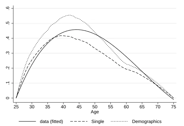
Figure 5: Household Consumption, Model vs. Data, OECD scale

0

.1

.2

.3

.4

.5

.6

25 30 35 40 45 50 55 60 65 70 75

Age

data (fitted) Single Demographics

Note: Calibration ofβ(discount factor) implies a value of 0.9889 and 0.9834 for theSingleandDemographics

models respectively.

using the profile for household size and composition in Figure2in conjunction with the appropriate

equivalence scale (i.e., ch = csφ(N) where ch is household consumption and cs is consumption

predicted from the single model). The Demographics model produces predictions for household

consumption directly, so we make no further adjustments. Below we present figures with results of

our exercises.

Figure 5 shows the results for our exercise using the OECD equivalence scale. In the figure we

compare the predictions for theSingleandDemographicsmodels versus the data. A striking feature

is the fact that our very simple quantitative framework is able to capture very well the hump shaped

profile of household consumption as seen in the data, hinting at the importance of family size and

composition in explaining the facts extracted from the CEX. This is basically the same result as

in Attanasio, Banks, Meghir, and Weber (1999). However, the fact that the quantitative model

lacks several mechanisms usually assumed in the literature (e.g. a realistic social security system,

transitory versus permanent income shocks, survival probabilities, a longer lifespan, among others)

hints that we might be attributing too much protagonism to household size. Although interesting,

the interaction between household size effects and these other modeling alternatives are beyond the

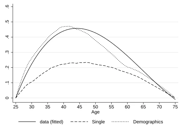
Figure 6: Household Consumption, Model vs. Data, Nelson scale

0

.1

.2

.3

.4

.5

.6

25 30 35 40 45 50 55 60 65 70 75

Age

data (fitted) Single Demographics

Note: Calibration ofβ(discount factor) implies a value of 0.9826 and 0.9809 for theSingleandDemographics

models respectively.

Our analysis confirms the result which we derived in the theoretical section: whether the model

incorporates economies of scale inside the problem of the agent (as in the Demographicsmodel) or

uses equivalence scales only as an accounting device (the Single case) matters for the size of the

predicted ’hump’ in household consumption. In the particular case of OECD scales, we see that

both models are relatively close, with theSinglemodel better predicting consumption up to age 40

and the Demographicsmodel, for ages 50 and older. We have to underscore once more the subtle

but important distinction between models: the Demographics model predicts higher household

consumption when household size is bigger because agents in that model are optimally choosing

consumption, given the price incentives introduced by changing economies of scale. In the Single

model, agents ignore these price effects. However, in the latter we get still a hump, since single

agents track income earlier in life (given the calibratedβ) and decrease consumption in retirement,

producing a non-demography related hump, to which consumption of additional equivalent adults

at certain points in the life-cycle are added to produce total household consumption. This can

be seen more clearly by comparing Figure 5 and Figure 10 (in the Appendix), where we present

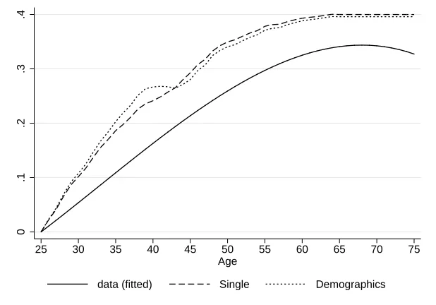
life-cycle profiles of per-adult equivalent consumption.

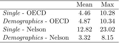
Table 2: Absolute percentage deviations of life-cycle consumption profiles with respect to US data

Mean Max

Single- OECD 4.46 10.28

Demographics- OECD 4.87 10.34

Single- Nelson 12.82 23.02

Demographics- Nelson 3.32 8.15

Note: The table shows the Mean and Maximum percentage differences between the predictions of theSingleand

Demographicsmodels for the profile of life-cycle household consumption, compared to the profile for US data from the CEX

discrepancy between models is substantial, with the Singlemodel vastly under predicting the size

of the ’hump’ in consumption over the life-cycle. On the other hand, theDemographicsmodel stays

on target, providing the best overall prediction across all models. The same result can be deduced

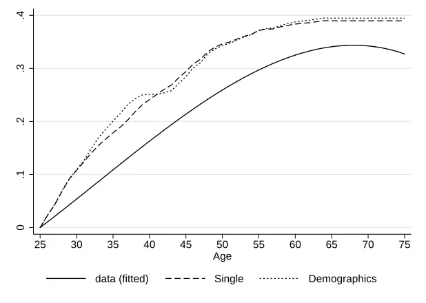
by comparing the per-adult equivalent profile from Figure11 in the Appendix.

The size of the gap between model predictions is related to the amount of economies of scale

implied by the equivalence scales. As we discussed earlier, the OECD scale implies very little

economies of scale inside the household, as opposed to what the Nelson scale prescribes.12 The

intuition is the following: if economies of scale are non-existent, living in a multi-person household

does not entail any gains nor savings in terms of public consumption. Mathematically, this is

represented by φ(N) = N, and from equation (7), we know that agents in the Demographics

model face the same relative prices as single individuals and the profiles of household consumption

coincide across models. On the other hand, if economies of scale in consumption are sizeable (i.e.,

φ(N) ≪ N) and the incentives to consume when household size is bigger are high (see again the

Euler equation in (7)). To be more specific, in Table2 we present the absolute difference between

the predictions from both models for the normalized life-cycle profiles of consumption versus the

same profile for US data. Since these predictions are in logs, these differences can be interpreted

as percentage deviations.

The main message from this section is that the single agent approach is bound to introduce

a heavy bias in terms of predictions for household consumption if economies of scale of living

together are high: if the gains for individuals of sharing a home are high, then we loose important

12_{From before, a household composed of two adults and two children is equivalent to 2.7 adults living alone}

Figure 7: Standard Deviation of log household consumption, OECD scale

0

.1

.2

.3

.4

25 30 35 40 45 50 55 60 65 70 75

Age

data (fitted) Single Demographics

information from modeling all agents as if they were bachelor/single households.

Result 2 of our theoretical model showed that as an implication of a pure accounting

exer-cise the discounted life-time per-adult equivalent consumption levels differ between the Singleand

Demographics model if household consumption and income in the Demographics model are not

fully synchronized. Our calculations show that under the proposed parameterization of the model,

present value of lifetime (per-adult equivalent) consumption is higher in theDemographicsthan in

theSinglemodel. The numbers are 2.4% when the OECD scale is used, versus 0.5% when it’s the

Nelson scale. The difference is smaller for the Nelson Scale because household consumption and

income are more synchronized over the life-cycle.

5.2 Consumption Inequality

In this section we compare the predictions with respect to life-cycle inequality. As before, we

consider the simulated sample of household consumption, from where we calculate the standard

deviation of log consumption at each age in the simulated life-cycles. The results are presented in

Figure 7and Figure 8.

From the figures we see that both models are able to replicate increasing consumption inequality

Figure 8: Standard Deviation of log household consumption, Nelson scale

0

.1

.2

.3

.4

25 30 35 40 45 50 55 60 65 70 75

Age

data (fitted) Single Demographics

this increase. We also see that the predictions of both theSingleandDemographicsmodel are very

close to each other, with no model having a clear edge in terms of closeness to the data. Around

ages 35 to 40, and for both equivalence scales, theDemographicsmodel has a small departure from

theSinglemodel, which is around the timing of the peak in household size.

6

Discussion: identifying the

Demographics

model

In this section we use estimates from Attanasio, Banks, Meghir, and Weber (1999) in order to

identify under which equivalence scale, the Demographics model is closest to the data. In other

words, we perform a simple test of how much economies of scale there exist. First, we take the

preferences used in Attanasio, Banks, Meghir, and Weber (1999):

u(c, Nad, Nch) = exp(ζ1Nad+ζ2Nch) c1−α

1−α, (24)

Given this utility function and the parameters ζ₁, ζ₂ and α obtained in that paper from an

Euler equation estimation (0.71, 0.34 and 1.57 respectively), we can make a simple comparison

Table 3: Empirical values for RHS of Equation (26)

Nad Nch N OECD NAS HHS DOC LM Nelson

2 0 2 0.75 0.77 0.86 0.88 0.98 0.98

2 1 3 0.60 0.63 0.70 0.73 0.82 0.87

2 2 4 0.56 0.60 0.66 0.66 0.80 0.88

2 3 5 0.57 0.63 0.67 0.67 0.82 0.95

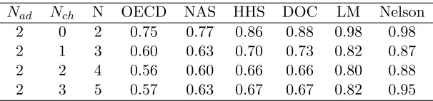
Note: Our considered equivalence scales are constructed respectively by the Organization for Economic Cooperation and Development (OECD), the National Academy of Sciences (NAS), the Department of Health and Human

Services (HHS), the Department of Commerce (DOC),Lazear and Michael(1980) andNelson(1993).

exp(ξ₁Nad+ξ2Nch) =

Nad+Nch φ(Nad, Nch)1−α

∀ Nad, Nch. (25)

For Nad = 1 and Nch = 0, our setup implies δ =φ = 1 whereas the preference parameter in

Attanasio, Banks, Meghir, and Weber(1999) is exp(ζ1). We therefore normalize the utility function

(24) by this number and rearrange (25) to obtain

1 = exp(ζ1[Nad−1] +ζ2Nch)φ(Nad, Nch)

1−α Nad+Nch

, (26)

an expression which does not necessarily hold empirically. In Table 3 we show the values for the

right hand side of (26) for the array of equivalence scales considered by Fern´andez-Villaverde and

Krueger(2007) and for different household arrangements, in terms of number of adults and children

present

The equivalence scales are displayed in increasing order of implied economies of scale: as

dis-cussed earlier, the OECD scale shows the smallest while the Nelson scale, the highest. Comparing

across columns, we see that under the latter, the empirical value of the right hand side of (26)

is closest to one, hence, the condition in that equation is most likely to hold. This independent

evidence validates our proposedDemographicsmodel when economies of scale are high (as implied

by the Nelson scale). As we showed above, this creates the biggest differences with the predictions

7

Conclusions

In this paper we suggest a simple framework to understand the sources of bias when single agent

models are used to make predictions for aggregate consumption or consumption related variables,

such as aggregate welfare.

Our proposedDemographicsmodel acknowledges that economies of scale in household

consump-tion (measured by equivalence scales, which are widely used in the quantitative literature) have an

effect on the agent’s perceived relative prices of consumption over the life-cycle when family size

and composition change. This is in stark contrast to the common practice of simulating a single

agent model, where these induced price effects are ignored. Hence, we find that economies of scale

in consumption inside the household are positively related to the bias introduced by the single

agent approach, given that in such a case the price effects are stronger.

We also perform a quantitative exercise and find that the single agent approach underestimates

the effect of family size on consumption over the life-cycle for mean consumption profiles but not

for inequality.

Finally, using estimates fromAttanasio, Banks, Meghir, and Weber(1999), we ask which

equiv-alence scale (or amount of economies of scale in the household) makes our model closest to the

em-pirical facts. We find that scales implying very high economies of scale do the job, which in turn,

References

Aguiar, M., and E. Hurst (2009): “Deconstructing Lifecycle Expenditure,” Working paper,

University of Rochester and University of Chicago.

Aiyagari, S. R., J. Greenwood, and N. Guner (2000): “On the State of the Union,” The

Journal of Political Economy, 108(2), pp. 213–244.

Attanasio, O. P., J. Banks, C. Meghir, and G. Weber (1999): “Humps and Bumps in

Lifetime Consumption,”Journal of Business & Economic Statistics, 17, 22–35.

Blundell, R., L. Pistaferri, and I. Preston (2008): “Consumption Inequality and Partial

Insurance,”American Economic Review, 98, 1887–1921.

Cubeddu, L., and J.-V. R´ıos-Rull (2003): “Families as Shocks,” Journal of the European

Economic Association, 1(2/3), pp. 671–682.

Deaton, A., and C. H. Paxson (1994): “Saving, Growth and Aging in Taiwan,” in Studies in

the Economics of Aging, ed. by D. A. Wise. Chicago University Press for the National Bureau of

Economic Research.

Fern´andez-Villaverde, J.,andD. Krueger(2007): “Consumption over the Life Cycle: Facts

from Consumer Expenditure Survey Data,” Review of Economics and Statistics, 89(3), 552–565.

(2010): “Consumption and Saving over the Life Cycle: How Important are Consumer

Durables?,” Macroeconomic Dynamics, Forthcoming.

Fuchs-Sch¨undeln, N.(2008): “The Response of Household Saving to the Large Shock of German

Reunification,”American Economic Review, 98(5), 1798–1828.

Gourinchas, P.-O.,andJ. A. Parker(2002): “Consumption over the life cycle,”Econometrica,

70, 47–89.

Gouveia, M., and R. Strauss(1994): “Effective Federal Individual Income Tax Functions: An

Exploratory Empirical Analysis,” National Tax Journal, 47(2), 317–339.

Guvenen, F., and A. A. Smith (2010): “Inferring Labor Income Risk from Economic Choices:

Heathcote, J., K. Storesletten, and G. L. Violante (2010): “The Macroeconomic

Im-plications of Rising Wage Inequality in the United States,” The Journal of Political Economy,

118(4), pp. 681–722.

Hong, J. H., and J.-V. R´ıos-Rull (2007): “Social security, life insurance and annuities for

families,” Journal of Monetary Economics, 54(1), 118 – 140, Carnegie-Rochester Conference

Series on Public Policy: Economic Consequences of Demographic Change in a Global Economy

April 21-22, 2006.

(2009): “Life Insurance and Household Consumption,” Working paper, University of

Rochester and University of Minnesota.

Kaplan, G., and G. L. Violante (2009): “How Much Consumption Insurance Beyond

Self-Insurance?,” Working paper, University of Pennsylvania and New York University.

Kopecky, K., and R. Suen (2010): “Finite State Markov-chain Approximations to Highly

Per-sistent Processes,”Review of Economic Dynamics, 13(3), 701–714.

Krueger, D., and F. Perri (2006): “Does Income Inequality Lead to Consumption Inequality?

Evidence and Theory.,” Review of Economic Studies, 73(1), 163 – 193.

Krueger, D., F. Perri, L. Pistaferri, andG. L. Violante(2010): “Cross-sectional facts for

macroeconomists,” Review of Economic Dynamics, 13(1), 1 – 14, Special issue: Cross-Sectional

Facts for Macroeconomists.

Lazear, E. P.,andR. T. Michael(1980): “Family Size and the Distribution of Real Per Capita

Income,” The American Economic Review, 70(1), pp. 91–107.

Mazzocco, M., C. Ruiz, and S. Yamaguchi (2007): “Labor Supply, Wealth Dynamics and

Marriage Decisions,” Mimeo.

Nelson, J. A.(1993): “Independent of a Base Equivalence Scales Estimation Using United States

Micro-Level Data,” Annales d’conomie et de Statistique, (29), pp. 43–63.

Storesletten, K., C. I. Telmer, andA. Yaron(2004): “Consumption and risk sharing over

Appendix

Additional Figures

Figure 9: Log of Nondurable Consumption, Relative to Age 25

0

.1

.2

.3

.4

.5

Log consumption, Raw vs. Adult Equivalent

25 30 35 40 45 50 55 60 65 70 75 Age

Figure 10: Adult Equivalent Consumption Relative to Age 25, OECD scale

0

.1

.2

.3

.4

.5

.6

25 30 35 40 45 50 55 60 65 70 75

Age

Single Demographics

Figure 11: Adult Equivalent Consumption Relative to Age 25, Nelson scale

0

.1

.2

.3

.4

.5

.6

25 30 35 40 45 50 55 60 65 70 75

Age

Single Demographics

Note: Model output in adult equivalent terms. TheSingle case shows directly the predictions from the respective

model. In theDemographicscase, predicted consumption is deflated by the corresponding equivalence scale (OECD