Optimization of hydroelectric power generation, case study of Roseires Dam in Sudan

Munich Personal RePEc Archive

Optimization of Hydroelectric Power

Generation, Case Study of Roseires Dam

in Sudan

Mohamed, Issam A.W.

Al Neelain University

2011

Online at

https://mpra.ub.uni-muenchen.de/31558/

1

Optimization of Hydroelectric Power Generation,

Case Study of Roseires Dam in Sudan

Professor Issam A.W. Mohamed ABSTRACT

Water reservoirs are large pools of water created stream or river catchment's areas and torrential rains and for storing water for use in many ways, and perhaps electric power generation is one of the most important uses of these reservoirs and for agriculture. That is extremely beneficial considering a rare and limited economic resources. Applied stochastic processes model has been applied in the work of Roseires dam, in order to develop a system to generate the highest possible power in the resources available. The current paper aims to apply another model, which is a dynamic programming model to verify the possibility of developing the same system and thus generate the highest possible electricity from the reservoir.

Data collected from the Ministry of Irrigation and the National Electricity Cooperation and international information network during the years 206-2007.

1.

Introduction

Studies take importance of water resources; the studies improvise mathematical models for designing and managing complicated systems, which involve many variables. One of studies deal with Dynamic programming models, and the goal of this study is to introduce Dynamic model for generating hydroelectric power. In 1952 Bellman introduced the theory of dynamic programming following that Young (1967) used the dynamic programming to obtain the optimal operation policy for multiple dams assumes the capacity of storage is known and the study had been applied in California. Mobashori (1970) developed Hall’s models to obtain better storage policy, but the use of stochastic dynamic programming started in 1955 by little. In (1973) Yeh applied the (S.D.P) for maximizing the generated power and in (1980) Dogli used (D.P) depended on forecast values for inputs.

2.

The Dynamic Model

The objective function is to achieve maximum production when operating the system, objective function of dams depends on standard for measuring the efficiency of dam for maximization.





 n

i n

P Max Z

1

 _where

n

P = Total of generated power subject to inputs, outflow, evaporation and other constraints

This objective function can be written as



 

 n

i n

j i in in Y h Y Max Z

1 1 , ,

Where

Sort of dam Constraint of mathematical model

Single Sn+1 = Sn + Xn – Yn – Dn - Vn

Two sequential dams S1,n+1 = S1,n + X1,n – Y1,n – 11,n - Yn,2 – V2,n

Multiple sequential dams Si,n+1 = Si,n + Xi,n + Yi–1,n – 1i,-1,n – Yi,n – Di,n – Vi,n Parallel dams Si,n+1 = Si,n + Xi,n – Yi,n – Di,n – Vi,n

Such that

Sn = Storage of water

Xn = Inputs of water

Yn = Output of water

Dn = Water had been taken from the Dam

Vn = Evaporation of water

3

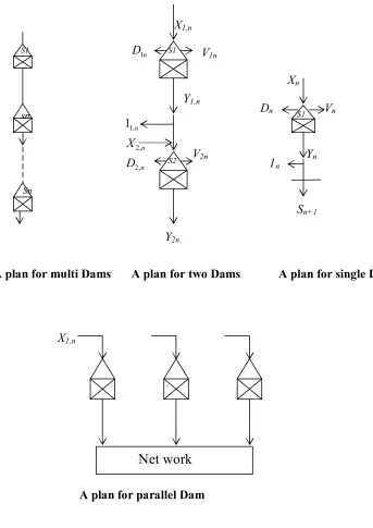
Figure (1) Plans for different dams S2

S1 S1

S1

sn

Sn

n D1

n n n

D X

, 2 , 2 , 1

1

X1,n

V1n

Y1,n

V2n

Y2n

Xn

Dn

1n

Sn+1 Vn

Yn

A plan for two Dams

A plan for multi Dams A plan for single Dams

A plan for parallel Dam

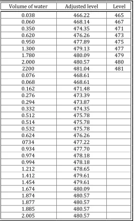
Table (1) The Adjusted levels of waters at Roseires dam

Volume of water Adjusted level Level

0.038 466.22 465

0.060 468.14 467

0.350 474.35 471

0.620 476.26 473

0.950 477.89 475

1.300 479.13 477

1.780 480.09 479

2.000 480.57 480

2200 481.04 481

0.076 468.61

0.068 468.61

0.162 471.48

0.276 473.39

0.294 473.87

0.332 474.35

0.512 475.78

0.514 475.78

0.532 475.78

0.624 476.26

0734 477.22

0.934 477.70

0.974 478.18

0.994 478.18

1.212 478.65

1.412 479.61

1.454 479.61

1.674 480.09

1.874 480.57

1.877 480.57

1.885 480.57

2.005 480.57

The (N.E.C) program was achieved by calculating the difference between the upper and lower levels, and then applied the equation as in their table, HEAD Vs. S.W.C (Specific Water Consumption).

Here we determine the differences between levels, which are the effected charge. In addition, the efficiency of turbines* water density*.

5

Table (2) Transformation of non linear for variables

Water

Volume Y Level X Log Y Log X

0.038 465 -3.270 6.142

0.060 467 -2.813 6.146

0.350 471 -1.050 6.155

0.620 473 -0.478 6.159

0.950 475 -0.051 6.163

1.30 477 0.262 6.167

1.78 479 0.577 6.171

2.00 480 0.693 6.173

2.200 481 0.788 6.176

When we apply the least squares estimation method for Log Y and Log X we get

 _{= 6.17 and}  _{= 0.0077}

Then 0077 . 0 0077 . 0 17 . 6 0077 . 0 17 . 6 0077 . 0 17 . 6

18

.

478

S

S

e

e

e

e

EL















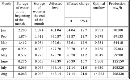
For the Rosiers dam, the generating electricity by the two methods is shown in the following tables

Table (3) Generating electricity by using stochastic process model Effected charge

Month Storage of water at the beginning of the month Storage of water at the end of the month Adjusted level

H S.W.C

Optimal

outflow Production mw/h

Jan 2.200 1.874 481.04 34.04 12.7 0.933 78188

Feb 1.874 1.412 480.57 33.57 12.7 0.878 69133

Mar 1.412 0.934 479.61 32.61 12.9 0.831 64418

Apr 0.934 0.532 477.70 30.70 13.2 0.730 55303

May 0.532 0.276 475.78 28.78 14.2 0.849 59788

June 0.276 0.068 473.39 26.39 15.7 1.808 115159

July 0.068 0.068 468.14 21.14 21.0 6.630 208320

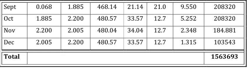
Sept 0.068 1.885 468.14 21.14 21.0 9.550 208320

Oct 1.885 2.200 480.57 33.57 12.7 5.252 208320

Nov 2.200 2.005 480.04 34.04 12.7 2.348 184.881

Dec 2.005 2.200 480.57 33.57 12.7 1.315 103543

Total 1563693

By using of dynamic programming model for the generation of electricity, we reach the results in the following table

Table (4) Generating electricity by using dynamic programming model Effected charge

Month Storage of water at the beginning of the month

Storage of water

at the end of the month

Adjusted level

H S.W.C

Optimal

outflow Production mw/h

Jan 2.200 1874 480.04 34.04 12.7 0.967 76141

Feb 1874 1.412 480.57 33.57 12.7 0.854 67244

Mar 1412 0.934 479.61 32.61 13.7 0.816 63750

Apr 0.934 0.532 477.70 30.70 14.2 0.716 52262

May 0.532 0.267 475.78 28.78 15.5 0.765 53873

June 0.276 0.068 473.39 26.39 21.0 1.755 113225

July 0.068 0.060 468.61 21.61 21.0 6.004 208320

Aug 0.060 0.060 468.14 21.14 21.0 14.424 208320

Sept 0.060 1.877 468.14 21.14 21.0 9.514 208320

Oct 1.877 2.200 480.57 33.57 12.7 6.232 208320

Nov 2.200 2.005 481.04 34.04 12.7 2.331 183543

Dec 2005 2.200 480.57 33.57 12.7 1.529 120393

Total 1563711

7

3.

Conclusion

The maximum production of electricity is achieved when 45–78% of the stored water used by using the pervious two models. Economic advantage is achieved here, especially under precious and rare single limited water source as in the case of the Nile River. Consideration should given to such a model as part of an optimum control paradigm. The National Electricity Authority is called for to consider the two mathematical models, stochastic or dynamic and more studies may be carried-out when the relation between the volume and the level of water is nonlinear.

4.

References

1. Betsekas, D.P. (1978) Dynamic Programming Deterministic and Stochastic Models.

New Jersey.

2. Cooper, L. & Cooper, M.W. (1991) Introduction to Dynamic Programming. Pergaman Press.

3. Druce, D.J. (1990) Incorporating Daily Flood Control objectives into a Monthly Stochastic Dynamic programming for a Hydroelectric complex. Water Resources. 26 (1).

4. Goulter, I.C. & Tai F.K. (1985) Practical Implications in the Use of Stochastic Dynamic

Programming for Reservoir Operation. Water Resources. 21 (1), 65 -74.

5. Kelman, J. et al (1990) Sampling Stochastic Dynamic Programming Applied to Reservoir Operation. Water Resources. 62 (3), 447 – 454.

6. Kelmes. V. (1974) Probability Distribution of Outflow from a linear Reservoir. Journal of Hydrology 21, 303.

7. Maidmenl, D. and Chow, V. (1981) Stochastic State Variable Dynamic Programming