Munich Personal RePEc Archive
Estimation in semiparametric models
with missing data
Chen, Songxi and Van Keilegom, Ingrid
December 2012
Estimation in semiparametric models
with missing data
∗
Song Xi
Chen
Guanghua School of Management and Center for Statistical Science
Peking University
Department of Statistics, Iowa State University
Ingrid
Van Keilegom
Institut de Statistique, Biostatistique et Sciences Actuarielles
Universit´e catholique de Louvain
October 20, 2012
Abstract
This paper considers the problem of parameter estimation in a general class of semiparametric models when observations are subject to missingness at random. The semiparametric models allow for estimating functions that are non-smooth with respect to the parameter. We propose a nonparametric imputation method for the missing values, which then leads to imputed estimating equations for the finite dimensional parameter of interest. The asymptotic normality of the parameter es-timator is proved in a general setting, and is investigated in detail for a number of specific semiparametric models. Finally, we study the small sample performance of the proposed estimator via simulations.
Key words: Copulas; imputation; kernel smoothing; missing at random; nuisance function; partially linear model; semiparametric model; single index model.
∗Chen acknowledges financial support from a National Science Foundation grant SES-0518904 and
1
Introduction
Semiparametric models encompass a large class of statistical models. They have the advantage of being more interpretable and parsimonious than nonparametric models, and at the same time they are less restrictive than purely parametric models. Let (X, Y) and (Xi, Yi), i = 1, . . . , n, be independent and identically distributed random vectors. We denote Θ for a finite dimensional parameter set (a compact subset of IRp) and H for a set of infinite dimensional functions depending on X and/or Y. The functions in H are allowed to depend on θ. Suppose that g(X, Y, θ, h) is an estimating function which is known up to the finite dimensional parameterθ ∈Θ and the infinite dimensional nuisance function h∈ H, and which satisfies
G(θ, h) := E{g(X, Y, θ, h)}= 0 (1.1)
atθ =θ0andh=h0, which are respectively the true parameter value and the true infinite
dimensional nuisance function.
Model (1.1) includes as special cases many well known semiparametric models. For instance, by adding a nonparametric functional component h(·) to the classical linear regression model, we get the following partially linear model :
Y =θTX1+h(X2) +ε, (1.2)
whereX = (X1, X2) is a covariate vector,Y is univariate response, and the errorεsatisfies
some identifiability constraint, like E(ε|X) = 0 or med(ε|X) = 0. Here h is a nuisance function that summarizes the nonparametric covariate effect due to a group of predictors
X2. In the context of the generalized linear model (McCullagh and Nelder, 1983), if the
known link function is replaced by an unknown nonparametric link function h, we arrive at the single-index regression model Y =h(θTX) +ε. Other semiparametric models that
are special cases of model (1.1) include copula models, semiparametric transformation models, Cox models, among many others.
Missing values are commonly encountered in statistical applications. In survey sam-pling e.g., there are typically non-responses of respondants to some survey questions. In biological applications, part of the data vector is often incompletely collected. The presence of missing values means that the entire sample {(Xi, Yi)}n
i=1 is not available.
a regression model, the vector Yi possibly contains some covariates, and the vector Xi
possibly contains the (or a) response.
There are basically two streams of inference methods for missing values. The first one is the imputation approach. The celebrated multiple imputation method of Little and Rubin (2002) is a popular representation of this approach. The idea of the second approach is based on inverse weighting by the missing propensity function proposed by James Robins and colleagues, see for instance Robins, Rotnitzky and Zhao (1994). The implementation of both approaches usually requires a parametric model for the missing propensity function or the missing at random mechanism (Rubin, 1976).
The aim of this paper is to provide a general estimator of the finite dimensional pa-rameter θ in the presence of the nuisance function h and of missing values. To make the estimation fully respective to the underlying missing values mechanism without assuming a parametric model, we impute for each missingYi multiple copies from a kernel estimator of the conditional distribution ofYi givenXi, under the assumption of missingness at ran-dom. This nonparametric imputation method can be viewed as a nonparametric counter part of the multiple imputation approach of Little and Rubin (2002). With the imputed missing values and a separate estimator for the nonparametric function h, the estimator of θ is obtained by solving an estimating equation based on (1.1). The consistency and asymptotic normality of the estimator are established under a set of mild conditions.
We end this section by mentioning some related papers on parametric and semipara-metric models with missing data. Recent contributions have been made e.g. by Wang, Wang, Gutierrez and Carroll (1998), Wang, Linton and H¨ardle (2004), M¨uller, Schick and Wefelmeyer (2006), Chen, Zeng and Ibrahim (2007), Wang and Sun (2007), Liang (2008), M¨uller (2009), Wang (2009) and Wang, Shen, He and Wang (2010). All these contri-butions are however limited to specific (often quite narrow) classes of models, whereas we aim in this paper at developing a general approach, applicable not only to regression models (with missing responses and/or covariates), but also to any other semiparametric model with missing data. We also refer to Chen, Hong and Tarozzi (2008), who study semiparametric efficiency bounds and efficient estimation of parameters defined through general moment restrictions with missing data. Their method relies however on auxiliary data containing information about the distribution of the missing variables conditional on proxy variables that are observed in both the primary and the auxiliary database, when such distribution is common to the two data sets.
framework are introduced in Section 2. Section 3 reports the general asymptotic result regarding the consistency and the asymptotic normality of the proposed estimator. The general result is illustrated and applied to a set of popular semiparametric models in Section 4. In Section 5 we study the small sample performance of the proposed estimator via simulations. All the technical details are provided in the Appendix.
2
General method
LetX be adx-dimensional vector that is always observable, and letY be ady-dimensional vector that is subject to missingness. Define ∆ = 1 if Y is observed, and ∆ = 0 if Y
is missing. We assume that Y is missing at random, i.e. ∆ and Y are conditionally independent given X :
P(∆ = 1|X, Y) = P(∆ = 1|X) =: p(X).
Note that using Y to denote the missing vector does not mean that we work under a regression model and that Y is the response in that model. SpecificiallyY can represent a set of covariates in a regression problem. Hence, our framework includes the case where the covariates are subject to missingness.
In the absence of missing values, the semiparametric model is defined by anr -dimensio-nal real valued estimation functiong(X, Y, θ, h), whereθ is a finite dimensional parameter taking values in a compact Θ ⊂ IRp, and h is an unknown function taking values in a functional space H (an infinite dimensional parameter set of functions) and is depending on X and/or Y. The functions in H are allowed to depend on θ too (but we will often suppress this dependence when no confusion is possible). Let θ0 and h0 be the true
unknown finite and infinite dimensional parameters. We often omit the arguments of the function h for notational convenience, i.e. (θ, h) ≡ (θ, hθ), (θ, h0) ≡ (θ, h0θ) and
(θ0, h0) ≡ (θ0, h0θ0). The estimating function g is known up to θ and h. Suppose that
r≥p, meaning that the number of estimating functions may be larger than the dimension of θ, so we allow for an over-identified set of equations, popular in e.g. econometrics. Moreover, by allowing the function g to be a non-smooth function of its arguments, our general model also includes e.g. quantile regression models or change-point models.
Let G(θ, h) = E[g(X, Y, θ, h)], which is a non-random vector-valued function G : Θ× H → IRr, such that G(θ, h0) = 0 for θ = θ0. If all data (Xi, Yi), i = 1, . . . , n
n−1Pn
i=1g(Xi, Yi, θ,bhθ), where bhθ is an appropriate estimator of hθ. See Chen, Linton
and Van Keilegom (2003) for more details.
The issue of interest here is the estimation of θ in the presence of missing values. Let (Xi,∆iYi,∆i), i = 1, . . . , n, be i.i.d. random vectors having the same distribution
as (X,∆Y,∆). We use a nonparametric approach to impute the missing values via a nonparametric kernel estimator ofF(y|x) = P(Y ≤y|X =x), the conditional distribution of Y given X =x. The kernel estimator of F(y|x) is
b
F(y|x) =
n
X
j=1
∆jKa(Xj −x)I(Yj ≤y)
Pn
l=1∆lKa(Xl−x)
, (2.1)
based on the portion of the sample without missing data, where K is a dx-dimensional
kernel function, a =an is a bandwidth sequence and Ka(·) =K(·/an)/adx
n .
For each missingYi, we generateκ(conditionally) independentY∗
i1, . . . , Yiκ∗ fromFb(·|Xi)
as imputed values for the missing Yi. Define now the imputed estimating function :
Gn(θ, h) = n−1 n
X
i=1
n
∆ig(Xi, Yi, θ, h) + (1−∆i)
1
κ κ
X
l=1
g(Xi, Yil∗, θ, h)
o
.
Note that the value of κ controls the variance of the imputed component. Theoretically speaking, we will let κ tend to infinity. Our numerical experience shows that the choice
κ= 50 is sufficient when the dimension is not too large. For larger dimension,κshould be chosen larger. We note that 1
κ
Pκ
l=1g(Xi, Yil∗, θ, h) approximates
R
g(Xi, y, θ, h)dFˆ(y|Xi). If the integral can be computed directly, then explicit imputation can be avoided. If a parametric model F(y|x;θ) is available for the conditional distribution, where θ is a finite dimensional parameter and ˆθ is its maximum likelihood estimator, then we can use F(y|x; ˆθ) instead of the nonparametric estimator ˆF(y|x) to generate the imputed Y∗
i .
We would like to emphasize here that our general model is not necessarily a regression model, and hence in general we cannot impute missing Y’s by using conditional mean imputation. And even if we would have a regression structure, the conditional mean imputation approach would still not be applicable in general, since Y does not necessarily represent the response variable in that model. See also Wang and Chen (2009), where a similar imputation approach has been used in the context of parametric estimating equations with missing values.
From the imputed estimating function Gn(θ, h) and for a given estimator bhθ of hθ, depending on the particular model at hand, we define the estimator of θ by :
b
where kAkW = (tr(ATW A))1/2 for any r-dimensional vector A and for some fixed
sym-metric r×r positive definite matrix W (and where tr stands for the trace of a matrix). Note that whenr=p(so the number of equations equals the number of parameters to be estimated) and when the function g is smooth inθ, the system of equationsGn(θ,bhθ) = 0 has a solution (namely θbdefined in (2.2)) under certain regularity conditions. In other situations (e.g. in the case of quantile regression or in an overidentified case), there is no vector θ that solves this equation, in which case we have to use the (more general) definition given in (2.2).
3
Main result
Below, we state the asymptotic normality of the estimatorθband we also give the formula of its asymptotic variance. The conditions under which this result is valid are given in the Appendix, and they will be checked in detail in Section 4 for a number of specific semiparametric models.
Theorem 3.1 Assume that conditions (A1)-(A5), (B1)-(B5) and (C1)-(C3) hold. Then,
b
θ−θ0 =n−1
n
X
i=1
(ΛTWΛ)−1ΛTW k(Xi,∆iYi,∆i) +oP(n−1/2),
and
n1/2(bθ−θ0)
d
→N(0,Ω),
where Ω = (ΛTWΛ)−1ΛTWVar{k(X,∆Y,∆)}WΛ(ΛTWΛ)−1,
k(x, δy, δ) = δ
p(x)g(x, y, θ0, h0) +
1− δ
p(x)
E[g(x, Y, θ0, h0)|X =x] +ξ(x, δy, δ),
the function ξ is defined in condition (A4), and Λ = Λ(θ0), with
Λ(θ) = d
dθG(θ, h0) = limτ→0
1
τ
h
G(θ+τ, h0,θ+τ)−G(θ, h0θ)
i
.
The proof of this result can be found in the Appendix.
Remark 3.2
(i) Instead of using an imputation approach to take care of the missing values, we could also estimateθ by minimizing
n−1
n
X
i=1
∆ig(Xi, Yi, θ,bh)
p(Xi,βb)
with respect to θ, where p(Xi) = p(Xi, β) follows e.g. a logistic model, and β can be estimated by
b
β = argmaxβ
n
X
i=1
∆ilogp(Xi, β) + (1−∆i) log(1−p(Xi, β)) .
See Robins, Rotnitzky and Zhao (1994), among many other papers, for more de-tails on this estimation procedure based on the inverse weighting by the missing propensity function.
(ii) Based on Theorem 3.1 the efficiency of the proposed estimator can be studied, and the optimal choice of the weight matrix W can be obtained. We do not elaborate on this in this paper, and refer e.g. to Section 6 in Ai and Chen (2003) for more details.
(iii) In the above i.i.d. representation ofθb−θ0, the function ξcomes from the estimation
of h0 bybh. Also, note that if there are no missing data, thenδ= 1 and p(·)≡1, so
k(x, δy, δ) = g(x, y, θ0, h0) +ξ(x, y,1) in that case.
(iv) Note that when r =p (i.e. there are as many equations as there are parameters to be estimated), then Ω reduces to
Ω = Λ−1Var{k(X,∆Y,∆)}(ΛT)−1,
provided Λ is of full rank.
4
Examples
4.1
Partially linear regression model
The first example we consider is that of a partial linear mean regression model :
Y =θTX1+h(X2) +ε, (4.1)
where E(ε|X) = 0, X = (XT
1, X2)T is (d+ 1)-dimensional, Y is one-dimensional and for
identifiability reasons we let E(h(X2)) = 0 (the linear part θTX1 contains an intercept).
We suppose that the responseY is missing at random. Let (X1, Y1), . . . ,(Xn, Yn) be i.i.d.
coming from model (4.1). Define g(x, y, θ, h) = (y−θTx
1−h(x2))x1, and let
bhθ(x2) =
n
X
i=1
Wni(x2, bn)
n
∆i[Yi−θTX1i] + (1−∆i)[mb(Xi)−θTX1i]
o
where
Wni(x2, bn) =
Lb(X2i−x2)
Pn
j=1Lb(X2j−x2)
,
L is a univariate kernel function, b =bn →0 is a bandwidth sequence, Lb(·) =L(·/b)/b, and mb(x) =R ydFb(y|x), with Fb(y|x) given in (2.1). Finally, let θb= argminθkGn(θ,bhθ)k, wherek · k is the Euclidean norm. Instead of working with the above estimator ofhθ(x2),
we could also work with a weighted average of the non-missing observations only.
We now verify conditions (A1)-(A5) and (B1)-(B5). Let h0θ(x2) = h0(x2) −(θ −
θ0)TE(X1|X2 =x2) =E(Y|X2 =x2)−θTE(X1|X2 =x2), and let khkH = supθ,x2|hθ(x2)|
for any h. First, note that
bhθ(x2)−h0θ(x2) =bhθ(x2)−E[bhθ(x2)|X] +
E[bhθ(x2)|X]−h0θ(x2)
= (T1+T2)(x2),
where X= (X1, . . . , Xn). Denoting Yie = ∆iYi+ (1−∆i)mb(Xi), we have thatE[Yie|X] = p(Xi)m(Xi) + (1−p(Xi))(m(Xi) +OP(aq
n)) =m(Xi) +oP(n−1/4) uniformly ini, provided na4q
n →0, and wherem(x) = E(Y|X =x) and q is the order of the kernel k. Hence, T1(x2) =
n
X
i=1
Wni(x2, bn)∆i[Yi−m(Xi)]
+
n
X
i=1
Wni(x2, bn)(1−∆i)[mb(Xi)−m(Xi)] +oP(n−1/4)
=OP((nbn)−1/2(logn)1/2) +OP((nand+1)−1/2(logn)1/2) +oP(n−1/4) =oP(n−1/4),
provided nb2
n(logn)−2 → ∞ and na
2(d+1)
n (logn)−2 → ∞. Next, consider T2(x2) =
n
X
i=1
Wni(x2, bn)[m(Xi)−θTX1i]−h0θ(x2) +oP(n−1/4)
=
n
X
i=1
Wni(x2, bn)[E(Y|Xi)−θTX1i−E(Y|X2i) +θTE(X1|X2i)]
+OP(b2n) +oP(n−1/4)
=OP((nbn)−1/2(logn)1/2) +oP(n−1/4) =oP(n−1/4),
uniformly in θ, provided nb8
n → 0. Hence, (A1) is verified. Next, for (A2), define H = C1
M(RX2), where the space C 1
(compact) support of X2. Using a similar derivation as for verifying condition (A1), we
can show that supkθ−θ0k=o(1)supx2|bh
′
θ(x2)−h′0θ(x2)|=oP(1), provided nb3n(logn)−1 → ∞, nad+1
n b2n(logn)−1 → ∞ and aqnbn−1 → 0. It then follows that P(bhθ ∈ CM1 (RX2)) → 1.
Moreover, the second part of (A2) is valid for s = 1 by Remark A.1. For condition (A3) note that for any θ and h, Γ(θ, h0)[h−h0] =−E{(hθ(X2)−h0θ(X2))X1}. Hence,
Γ(θ, h0)[bh−h0]−Γ(θ0, h0)[bh−h0]
=(θ−θ0)TE
nhXn i=1
Wni(X2, bn)X1i−E(X1|X2)
i
X1o=oP(kθ−θ0k).
Next, consider (A4). Using the above derivations, write
b
hθ0(x2)−h0(x2)
=
n
X
i=1
Wni(x2, bn)
h
∆i{Yi−m(Xi)}+ (1−∆i){mb(Xi)−m(Xi)}
i
+oP(n−1/2),
provided na2q
n → 0 and nb4n → 0. Replacing Wni(x2, bn) by (nbn)−1K(X2bi−nx2)/fX2(x2), and noting that
b−n1En X1 fX2(X2)
KX2i−X2 bn
o
=E(X1|X2 =X2i) +O(b2n),
uniformly in i, we obtain
Γ(θ0, h0)[bh−h0] =−E{(hbθ0(X2)−h0(X2))X1}
=−n−1 n
X
i=1
E(X1|X2i)
h
∆i{Yi−m(Xi)}+ (1−∆i){mb(Xi)−m(Xi)}
i
+oP(n−1/2).
It can be easily seen that
n−1 n
X
i=1
E(X1|X2i)(1−∆i){mb(Xi)−m(Xi)}
=n−1 n
X
i=1
1−p(Xi)
p(Xi) E(X1|X2i)∆i{Yi−m(Xi)}+oP(n
−1/2),
and hence
ξ(Xi,∆Yi,∆i) =−E(X1|X2i)
∆i
For (A5) consider
Gn(θ, h)−Gne (θ, h) =n−1 n
X
i=1
(1−∆i)
h1
κ κ
X
l=1
Yil∗ −E(Y|X =Xi)iX1i
=n−1 n
X
i=1
(1−∆i)
b
m(Xi)−m(Xi)X1i+oP(1) =oP(1),
as κ and n tend to infinity. Since this does not depend on θ, the second part of (A5) is obvious.
We now turn to the B-conditions. Condition (B1) is an identifiability condition, whereas (B2) holds true provided E|X1j| < ∞ for j = 1, . . . , d. Next, for (B3) it is
easily seen that
Λ =−Eh(X1−E(X1|X2))TX1
i
=−Var[X1|X2],
which we assume to be of full rank. Condition (B4) is automatically fulfilled sinceG(θ, h) is linear in h. Finally, condition (B5) holds true for s= 1.
It now follows from Theorem 3.1 that n1/2(bθ −θ
0) is asymptotically normally
dis-tributed with asymptotic variance given by
Ω = Λ−1Varh ∆
p(X){Y −θ
T
0X1−h0(X2)}{X1−E(X1|X2)}
i
(ΛT)−1,
since E[g(x, Y, θ0, h0)|X =x] = 0. Note that if all data would be observed, the matrix Ω
equals the variance-covariance matrix given in Robinson (1988), who considers the special case where ε is independent of X.
4.2
Single index regression model
We now consider a single index regression model :
Y =h(θTX) +ε, (4.2) where X is d-dimensional, Y is one-dimensional, E(ε|X) = 0 and θ ∈ Θ = {θ ∈ IRd : kθk = 1} for identifiability reasons. See Powell, Stock and Stoker (1989), Ichimura and Lee (1991), Ichimura (1993), H¨ardle, Hall and Ichimura (1993), among many others for important results on the estimation and inference for this model when all the data are completely observed. We assume here that the responseY is missing at random. Suppose that the density of θT
to be compact). Let (X1, Y1), . . . ,(Xn, Yn) be a sample of i.i.d. data drawn from model
(4.2). Define g(x, y, θ, h, h′) = (y−h(θTx))h′(θTx)x, and let
b
hθ(u) =
n
X
j=1
Wnj(u)Yj
be a kernel estimator ofh0θ(u) =E(Y|θTX =u), where Wnj(u) = ∆jLb(θ
TXj−u)
Pn
ℓ=1∆ℓLb(θTXℓ−u)
,
L is a kernel function and b is an appropriate bandwidth. Finally, let θbbe a solution of the equation Gn(θ,bhθ,bh′
θ) = 0.
We restrict attention here to the calculation of the matrix Λ and the function ξ, which determine the asymptotic variance of θb. The verification of conditions (A1)-(A5) and (B1)-(B5) can be done by adapting the arguments used in the previous example to the context of single index models. Details are omitted. Note that
Λ = d
dθE
h
(Y −h0θ(θTX))h′0θ(θTX)Xi θ=θ0
.
It can be easily seen that Λ can also be written as
Λ =−Ehh′02(θ0TX){X−µX(θ0TX)}{X−µX(θT0X)}Ti,
where µX(u) = E(X|θT
0X =u). Also note that
Γ(θ0, h0)[h−h0, h′−h′0] =−E
h
{hθ0(θ
T
0X)−h0(θ0TX)}h′0(θT0X)X
i
+Eh{Y −h0(θT0X)}{h′θ0(θ
T
0X)−h′0(θ0TX)}X
i
.
Since the latter term equals zero, we have that
Γ(θ0, h0)[bh−h0,bh′−h′0]
=−n−1 n
X
i=1
∆i p(Xi)
{Yi−h0(θT0Xi)}h′0(θT0Xi)E(X|θ0TX =θT0Xi) +oP(n−1/2).
It now follows that the asymptotic variance of θbequals
Ω = Λ−1Varh ∆
p(X){Y −h0(θ
T
0X)}h′0(θT0X){X−E(X|θT0X)}
i
(ΛT)−1.
4.3
Copula model
In the third example we consider a copula model for two random variablesX andY, with
X being always observed and Y being missing at random. We suppose that the copula belongs to a parametric family {Cθ :θ ∈ Θ} where Θ is a subset of IRp. Hence, for any
x, y,
F(x, y) =P(X ≤x, Y ≤y) =Cθ(FX(x), FY(y)),
where FX(x) = P(X ≤x) and FY(y) = P(Y ≤y) are the marginals of X and Y, which are completely unspecified and will be estimated nonparametrically. We assume that FX
and FY are continuous, so that θ0 is unique. Let (Xi, Yi), i = 1, . . . , n be i.i.d. with
common distribution F. Define FXb (x) = (n+ 1)−1Pn
i=1I(Xi ≤x) and
b
FY(y) = (n+ 1)−1
n
X
i=1
n
∆iI(Yi ≤y) + (1−∆i)Fb(y|Xi)
o
,
where Fb(y|x) is defined in (2.1). Note that in a second step the estimator FYb (y) could be improved, by replacing Fb(y|x) by Fθb(y|x) = C2
θ(FXb (x),FYb (y)), whereCθ2 denotes the
derivative ofCθ with respect to the second argument (similar notations are used to denote
higher order derivatives). In what follows we restrict attention to the estimator defined in the first step. Now, define
g(x, y, θ, FX, FY) = C12′
θ (FX(x), FY(y)) C12
θ (FX(x), FY(y))
(the prime in C12′
θ stands for the derivative with respect to θ), i.e. g(x, y, θ, FX, FY) is
the derivative of the log-likelihood function under the copula model, and define bθ = argminθ∈ΘkGn(θ,FXb ,FYb )k.
We now calculate the function ξ defined in condition (A4), from which the formula of the asymptotic variance of θbcan be easily obtained. We omit the verification of the conditions of Theorem 3.1, but more details can be obtained from the authors. Let
dθ(u, v) =C12′
θ (u, v)/Cθ12(u, v). Then, straightforward calculations show that
Γ(θ, FX, FY)[FXb −FX,FYb −FY] =Eh ∂
∂udθ(u, FY(Y))|u=FX(X)(FXb (X)−FX(X)) + ∂
∂vdθ(FX(X), v)|v=FY(Y)(FbY(Y)−FY(Y))
i
Next, note that
b
FY(y)−FY(y) =n−1 n
X
i=1
h
∆iI(Yi ≤y) + (1−∆i)F(y|Xi)−FY(y)
i
+n−1 n
X
i=1
(1−∆i)
h b
F(y|Xi)−F(y|Xi)
i
.
For the second term above it can be shown that
n−1 n
X
i=1
(1−∆i)E
h ∂
∂vdθ(FX(X), v)|v=FY(Y)(Fb(Y|Xi)−F(Y|Xi))
i
=n−1 n
X
i=1
1−p(Xi) p(Xi) E
h ∂
∂vdθ(FX(X), v)|v=FY(Y)(I(Yi ≤Y)−F(Y|Xi))
i
+oP(n−1/2).
It now follows that
Γ(θ0, FX, FY)[FXb −FX,FYb −FY]
=n−1 n
X
i=1
Eh ∂
∂udθ0(u, FY(Y))|u=FX(X)
n
I(Xi ≤X)−FX(X)o
+ ∂
∂vdθ0(FX(X), v)|v=FY(Y)
n
∆iI(Yi ≤Y) + (1−∆i)F(Y|Xi)−FY(Y)
+1−p(Xi)
p(Xi) (I(Yi ≤Y)−F(Y|Xi))
oi
+oP(n−1/2).
The formula of the asymptotic variance can now be easily obtained from Theorem 3.1.
5
Simulation study
In this section we present simulation results for a single index mean regression model. Consider
Y =h(θTX) +ε,
where X = (X1, X2, X3)T, Xj ∼ Unif[0,1] (j = 1,2,3), (X1, X2, X3) are mutually
in-dependent, ε ∼ N(0,0.52), θ ∈ Θ = {θ ∈ IR3 : kθk = 1}, and h(u) = exp(u). The
probability that the response Y is missing depends on the covariate X via a logistic model :
P(∆ = 1|X, Y) = exp(β
TX)
1 + exp(βTX).
replace θ, i.e. we write θ(α) = (sin(α1) sin(α2),sin(α1) cos(α2),cos(α1))T for some α1, α2.
Note thatkθk= 1 for any value ofα1 andα2. In the simulations, we work withα1 =π/3
and α2 =π/6, and we take β = (1,1,0)T in Table 1, andβ = (0.5,0.5,0)T in Table 2.
The estimating function for α1 and α2 is given by
g(x, y, α, h)
=ny−h(θ(α)Tx)oh′(θ(α)Tx) cos(α1) sin(α2)x1+ cos(α1) cos(α2)x2 −sin(α1)x3 sin(α1) cos(α2)x1−sin(α1) sin(α2)x2
!
.
Next, definebh(u) =Pnj=1Wnj(u)Yj, where
Wnj(u) = ∆jKb(u−θ(α)
TX j)
Pn
i=1∆iKb(u−θ(α)TXi)
.
The imputed estimating equation is
Gn(α, h) =n−1 n
X
i=1
h
∆ig(Xi, Yi, α, h) + (1−∆i)
1
κ κ
X
l=1
g(Xi, Yil∗, α, h)i. (5.1)
We now define αb as the solution of the equation Gn(α,bh) = 0 with respect to all vectors
α∈[0,2π]2. Throughout the simulation k was set to be 50.
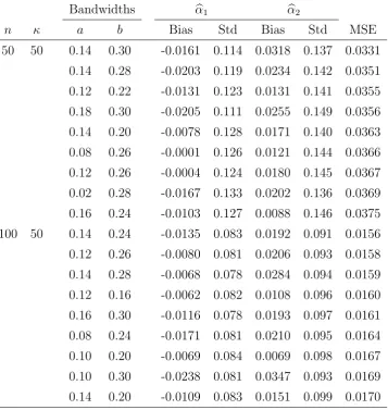
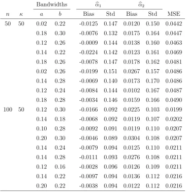
Two bandwidths need to be selected. The first one is the bandwidth a in the kernel estimator of the conditional distribution functionF(y|x) defined in (2.1), which is used for the imputation procedure. The second one is in the bandwidth b in the kernel estimator of the function h. Because the cross-validation method for selecting bandwidths is com-plicated when imputation is involved, and because it can only produce one combination of bandwidths, we prefer to use a sequence of bandwidths for aand b to study the influence of the bandwidths on the estimator. In our simulation, we considered for a and b all values between 0.02 and 0.30 with step size 0.02. We so obtain 225 combinations of the bandwidths used for estimating α. We report in Tables 1 and 2 the results corresponding to the 9 pairs of bandwidths a and b that lead to the smallest MSEs.
Table 1 summarizes the bias, standard deviation and MSE of the estimators of α1 and
α2 based on the selected a and b. The MSE is the sum of the MSEs of αb1 and αb2. Each
entry is based on 500 simulations. The table shows that the influence of the bandwidth is rather small. We also notice that the bias is reasonably close to 0 and as the sample size increases, the standard deviation and MSE of αb1 and αb2 decrease. In Table 2 the
Appendix
Below we list the assumptions that are needed for the main result in Section 3. The following notations are needed. We equip the spaceHwith a semi-normk · kH, defined by
khkH = supθ∈ΘkhθkSfor anyh ∈ H, i.e.k·kHis a sup-norm with respect to theθ-argument
and a semi-normk · kS with respect to all the other arguments. Also,N(λ,H,k · kH) is the
covering number of the class H with respect to the norm k · kH, i.e. the minimal number
of balls of k · kH-radius λ needed to coverH. We use the notation Λ(θ) = dθdG(θ, h0) to
denote the complete derivative ofG(θ, h0) with respect to θ, i.e.
Λ(θ) = d
dθG(θ, h0) = limτ→0
1
τ
h
G(θ+τ, h0,θ+τ)−G(θ, h0θ)
i
, (A.1)
and the notation Γ(θ, h0)[h−h0] to denote the functional derivative of G(θ, h0) in the
direction [h−h0], i.e.
Γ(θ, h0)[h−h0] = lim
τ→0
1
τ
h
G(θ, h0 +τ(h−h0))−G(θ, h0)
i
.
We also need to introduce the function
e
Gn(θ, h) =n−1 n
X
i=1
[∆ig(Xi, Yi, θ, h) + (1−∆i)E{g(Xi, Y, θ, h)|X =Xi}].
Finally, k · k denotes the Euclidean norm.
Assumptions on the estimator bh
(A1) supθ∈Θkbhθ−h0θkS =oP(1), and supkθ−θ0k≤δnkbhθ−h0θkS =oP(n
−1/4), whereδn →0,
and where h0θ is such that h0θ0 ≡h0.
(A2) P(bhθ ∈ H)→1 asn tends to infinity, uniformly over allθ withkθ−θ0k=o(1), and
R∞
0
p
logN(λ1/s,H,k · k
H)dλ <∞, where 0< s≤1 is defined in condition (B5).
(A3) Forθ in a neighborhood ofθ0,kΓ(θ, h0)[bh−h0]−Γ(θ0, h0)[bh−h0]kW =oP(kθ−θ0k).
(A4) Γ(θ0, h0)[bh−h0] = n−1Pni=1ξ(Xi,∆iYi,∆i) +oP(n−1/2), where the function ξ =
(ξ1, . . . , ξr) satisfies E[ξj(X,∆Y,∆)] = 0 and E[ξj2(X,∆Y,∆)]<∞forj = 1, . . . , r.
(A5) supθ∈ΘkGn(θ,bh)−Gne (θ,bh)kW =oP(1), and for any δn→0,
sup
kθ−θ0k≤δn
Assumptions on the function G
(B1) For all δ >0, there exists ǫ >0 such that infkθ−θ0k>δkG(θ, h0)kW ≥ǫ >0.
(B2) Uniformly for all θ ∈ Θ, G(θ, h) is continuous in h with respect to the k · kH-norm
ath=h0.
(B3) The matrix Λ(θ) exists for θ in a neighborhood of θ0, and is continuous at θ =θ0.
Moreover, Λ≡Λ(θ0) is of full rank.
(B4) For all θ in a neighborhood of θ0, Γ(θ, h0)[h−h0] exists in all directions [h−h0],
and for some 0< c <∞, kG(θ, h)−G(θ, h0)−Γ(θ, h0)[h−h0]kW ≤ckh−h0k2H.
(B5) For each j = 1, . . . , r,
Eh sup
(θ′,h′):kθ′−θk≤δ,kh′−hk H≤δ
|gj(X, Y, θ′, h′)−gj(X, Y, θ, h)|2
i
≤Kδ2s,
for all (θ, h)∈Θ× Hand δ >0, and for some constants 0< K < ∞and 0< s≤1.
Regularity assumptions
(C1) The kernel K satisfiesK(u1, . . . , udx) =
Qdx
j=1k(uj), where k is a qth-order (q≥ 2)
univariate probability density function supported on [−1,1], and k is bounded, symmetric and Lipschitz continuous. The bandwidth an satisfies nadx
n → ∞ and na2q
n →0. Moreover,κ→ ∞.
(C2) For all x0 ∈ X and θ ∈Θ, the function x→ E[gℓ(x0, Y, θ, h0)|X = x] is uniformly
continuous inx for ℓ= 1 and 2, and E[g2(X, Y, θ, h
0)]<∞.
(C3) For all x0 ∈ X and θ ∈ Θ, the functions x → p(x), fX(x), mg(x0, x, θ, h0) and
mg2(x0, x, θ, h0) are q times continuously differentiable with respect to the
compo-nents of xon the interior of their support. Here,fX is the probability density func-tion ofX and mgℓ(x0, x, θ, h) = E[gl(x0, Y, θ, h)|X =x]. Moreover, infx∈Xp(x)>0.
Remark A.1 Suppose the functions in H have a compact support R of dimension d ≤
dx +dy. In order to check condition (A2), define for any vector a = (a1, . . . , ad) of d
integers, the differential operator
Da= ∂
|a|
∂ua1 1 . . . ∂u
ad
where |a| =Pdi=1ai. For any smooth function h: R →IR and some α > 0, let α be the largest integer smaller than α, and
khk∞,α= max
|a|≤αsupu
|Dah(u)|+ max
|a|=αusup6=u′
|Dah(u)−Dah(u′)|
ku−u′kα−α .
Further, let Cα
M(R) be the set of all continuous functions h: R →IR with khk∞,α ≤ M.
If H ⊂Cα
M(R) with k · kH =k · k∞, then logN(λ,H,k · k∞)≤K(M/λ)d/α, whereK is a
constant depending only on d, α and the Lebesgue measure of the domain R. Hence,
Z ∞
0
q
logN(λ1/s,H,k · k
∞)dλ <∞ if α >
d
2s
(see Theorem 2.7.1 in Van der Vaart and Wellner (1996)).
Proof of Theorem 3.1. The proof is based on Theorems 1 and 2 in Chen, Linton and
Van Keilegom (2003) (CLV hereafter). In these theorems high-level conditions are given under which the estimatorθbis, respectively, weakly consistent and asymptotically normal. We start with verifying the conditions of Theorem 1 in CLV. Condition (1.1) holds by definition ofθb, while the second, third and fourth condition are guaranteed by assumptions (B1), (B2) and (A1). Finally, condition (1.5) can be treated in a similar way as condition (2.5) of Theorem 2 of CLV, which we check below. Next, we verify conditions (2.1)–(2.6) of Theorem 2 in CLV. Condition (2.1) is, as for condition (1.1), valid by construction of the estimator bθ. For (2.2) and the first part of (2.3), use assumptions (B3) and (B4). For the second part of (2.3), it follows from the proof in CLV that it suffices to assume (A3). Next, for condition (2.4), we use assumptions (A1) and (A2). For (2.5), note that
kGn(θ, h)−G(θ, h)−Gn(θ0, h0) +G(θ0, h0)kW
≤ kGn(θ, h)−Gne (θ, h)−Gn(θ0, h0) +Gne (θ0, h0)kW
+kGne (θ, h)−G(θ, h)−Gne (θ0, h0) +G(θ0, h0)kW.
For the first term above, note that it follows from the proof of Theorem 2 in CLV that it suffices to take h =bh. Hence, assumption (A5) gives the required rate. For the second term we verify the conditions of Theorem 3 in CLV. For condition (3.2) note that for
j = 1, . . . , r and for fixed (θ, h)∈Θ× H,
Ehsup∗∆gj(X, Y, θ′, h′)−∆gj(X, Y, θ, h)−(1−∆)E{gj(X, Y, θ′, h′)|X}
+(1−∆)E{gj(X, Y, θ, h)|X}i
where sup∗ is the supremum over all kθ′ −θk ≤ δn and kh′ −hk
H ≤ δn, with δn → 0.
Hence, condition (3.2) follows from assumption (B5), whereas condition (3.3) is given in (A2). Finally, condition (2.6) is valid by combining assumption (A4), Proposition A.1
and the central limit theorem.
Proposition A.1 Assume that conditions (A1)-(A5), (B1)-(B5) and (C1)-(C3) hold.
Then,
Gn(θ0, h0) =n−1
n
X
i=1
n ∆i
p(Xi)g(Xi, Yi, θ0, h0) +
1− ∆i
p(Xi)
E[g(Xi, Y, θ0, h0)|X =Xi]
o
+oP(n−1/2).
Proof. First we consider
Gn(θ0, h0)−Gne (θ0, h0)
=n−1 n
X
i=1
(1−∆i)
n1
κ κ
X
l=1
g(Xi, Yil∗, θ0, h0)−mgae (Xi, θ0, h0)
o
+n−1 n
X
i=1
(1−∆i)
n e
mga(Xi, θ0, h0)−mg(Xi, θ0, h0)
o
:=Vn1(θ0, h0) +Vn2(θ0, h0),
where mg(x, θ0, h0) = E[g(x, Y, θ0, h0)|X =x] and
e
mga(x, θ0, h0) =
n
X
j=1
∆jKa(Xj −x)
Pn
l=1∆lKa(Xl−x)
g(x, Yj, θ0, h0)
is the conditional mean imputation based on the kernel estimator of the conditional dis-tribution. We will first show that Vn1(θ0, h0) =oP(n−1/2), which means that we can just
substitute κ−1Pκ
l=1g(Xi, Yil∗, θ0, h0) by the conditional mean imputation mgae (Xi, θ0, h0),
which would simplify the theoretical analysis. However, the proposed imputation is at-tractive in practical implementations as it separates the imputation and analysis steps, as proposed by Little and Rubin (2002). Let χnc = {(Xj, Yj,∆j = 1) : j = 1, . . . , n} be
the complete part of the sample with no missing values. Given Xi with ∆i = 0, write
b
mgκ(Xi, θ0, h0) =κ−1Pκl=1g(Xi, Yil∗, θ0, h0). From the way we impute Yil∗,
Hence, E{Vn1(θ0, h0)}= 0. We next calculate the variance of Vn1(θ0, h0). Note that
Var{Vn1(θ0, h0)}=n−2
n
X
i,j
Covn(1−∆i)[mgκb (Xi, θ0, h0)−mgae (Xi, θ0, h0)],
(1−∆j)[mbgκ(Xj, θ0, h0)−mega(Xj, θ0, h0)]
o
.
If i6=j, then conditioning on χnc, (Xi,∆i = 0) and (Xj,∆j = 0),
Covh{mgκb (Xi, θ0, h0),mgκb (Xj, θ0, h0)}|χnc,(Xi,∆i = 0),(Xj,∆j = 0)
i
= 0.
This together with (A.2) implies that
Var{Vn1(θ0, h0)} (A.3)
=n−2 n
X
i=1
Varn(1−∆i)[mgκb (Xi, θ0, h0)−mgae (Xi, θ0, h0)]
o
=n−1EhVarnmgκb (Xi, θ0, h0)−mgae (Xi, θ0, h0)|χnc,(Xi,∆i = 0)
oi
= (nκ)−1EhP n
l=1∆lKaP(Xl−Xi)(ggT)(Xi, Yl, θ0, h0)
n
l=1∆lKa(Xl−Xi)
−(mgae meTga)(Xi, θ0, h0)
i
=O{(nκ)−1}, (A.4)
provided (C2) and (C3) hold true. Hence, Vn1(θ0, h0) =oP(n−1/2). Next, we consider the
term Vn2(θ0, h0). Defining wj(x, a) = ∆jKa(Xj −x)/{Pnl=1∆lKa(Xl−x)}, we have,
Vn2(θ0, h0) =n−1
n
X
i=1
(1−∆i) n
X
k=1
wk(Xi, a)ng(Xi, Yk, θ0, h0)−mg(Xi, θ0, h0)
−g(Xk, Yk, θ0, h0) +mg(Xk, θ0, h0)
o
+n−1 n
X
i=1
(1−∆i) n
X
k=1
wk(Xi, a)ng(Xk, Yk, θ0, h0)−mg(Xk, θ0, h0)
o
=Vn21(θ0, h0) +Vn22(θ0, h0).
First, we will show that Vn21(θ0, h0) = oP(n−1/2). Note that E[Vn21(θ0, h0)] = 0 and using
the notation
γnj(x1, x2) = (1−p(x1))(1−p(x2))Cov[g(x1, Yj, θ0, h0)−g(Xj, Yj, θ0, h0),
we have,
Var[Vn21(θ0, h0)] =E
n
Var[Vn21(θ0, h0)|X1, . . . , Xn]
o
=n−2 n
X
i,j,k=1
Enwj(Xi, a)wj(Xk, a)γnj(Xi, Xk)o
=n−2 n
X
i,j,k=1
Enwj(Xi, a)wj(Xk, a)γnj(Xj, Xj)
o
+O(n−1aqn)
=O(n−1aqn),
since γnj(Xj, Xj) = 0. Hence, Vn21(θ0, h0) =oP(n−1/2). Next, note that
Vn22(θ0, h0) =n−1
n
X
i=1
∆i{g(Xi, Yi, θ0, h0)−mg(Xi, θ0, h0)}
1−p(Xi)
p(Xi) +oP(n
−1/2),
where the rate of the remainder term can be shown in a similar way as for Vn21(θ0, h0).
This shows that
Gn(θ0, h0)
=Gne (θ0, h0) +
h
Gn(θ0, h0)−Gne (θ0, h0)
i
=n−1 n
X
j=1
[∆jg(Xj, Yj, θ0, h0) + (1−∆j)mg(Xj, θ0, h0)]
+n−1 n
X
j=1
∆j[g(Xj, Yj, θ0, h0)−mg(Xj, θ0, h0)]
1−p(Xj)
p(Xj)
+oP(n−1/2)
=n−1 n
X
j=1
h ∆j
p(Xj)g(Xj, Yj, θ0, h0) +
1− ∆j
p(Xj)
mg(Xj, θ0, h0)
i
+oP(n−1/2).
References
Ai, C. and Chen, X. (2003). Efficient estimation of models with conditional moment restrictions containing unknown functions. Econometrica, 71, 1795-1843.
Chen, X., Linton, O.B. and Van Keilegom, I. (2003). Estimation of semiparametric models when the criterion function is not smooth. Econometrica, 71, 1591-1608.
Chen, Q., Zeng, D. and Ibrahim, J.G. (2007). Sieve maximum likelihood estimation for regression models with covariates missing at random. J. Amer. Statist. Assoc., 102, 1309-1317.
H¨ardle, W., Hall, P. and Ichimura, H. (1993). Optimal smoothing in single-index models. Ann. Statist., 21, 157-178.
Ichimura, H. (1993). Semiparametric least squares (SLS) and weighted SLS estimation of single-index models. J. Econometrics, 58, 71–120.
Ichimura, H. and Lee, L.-F. (1991). Semiparametric least squares estimation of multiple index models: single equation estimation. In: Barnett, W.A., Powell, J. and Tauchen, G. (Eds.),Nonparametric and Semiparametric Methods in Statistics and Econometrics. Cambridge University Press, Cambridge. (Chapter 1).
Liang, H. (2008). Generalized partially linear models with missing covariates. J. Multiv. Anal.,99, 880-895.
Little, R.J.A. and Rubin, D.B. (2002). Statistical Analysis with Missing Data, Wiley. McCullagh, P. and Nelder, J.A. (1983). Generalized Linear Models. Chapman & Hall,
London.
M¨uller, U.U. (2009). Estimating linear functionals in nonlinear regression with responses missing at random. Ann. Statist.,37, 2245-2277.
M¨uller, U.U., Schick, A. and Wefelmeyer, W. (2006). Imputing responses that are not missing. Probability, Statistics and Modelling in Public Health (M. Nikulin, D. Com-menges and C. Huber, eds.), 350-363, Springer.
Powell, J.L., Stock, J.M. and Stoker, T.M. (1989). Semiparametric estimation of index coefficients. Econometrica, 57, 1403–1430.
Robins, J.M., Rotnitzky, A. and Zhao, L.P. (1994). Estimation of regression coefficients when some regressors are not always observed. J. Amer. Statist. Assoc., 89, 846-866. Robinson, P.M. (1988). Root-N-consistent semiparametric regression. Econometrica,56,
931-954.
Rubin, D.B. (1976). Inference and missing values (with discussion). Biometrika, 63, 481-592.
Van der Vaart, A.W. and Wellner, J.A. (1996). Weak Convergence and Empirical Pro-cesses. Springer-Verlag, New York.
for generalized linear models with missing data. Ann. Statist., 26, 1028-1050.
Wang, D. and Chen, S.X. (2009). Empirical likelihood for estimating equations with missing values. Ann. Statist., 37, 490-517.
Wang, Q.-H. (2009). Statistical estimation in partial linear models with covariate data missing at random. Ann. Inst. Statist. Math.,61, 47-84.
Wang, Q., Linton, O. and H¨ardle, W. (2004). Semiparametric regression analysis with missing response at random. J. Amer. Statist. Assoc., 99, 334-345.
Wang, Q. and Sun, Z. (2007). Estimation in partially linear models with missing responses at random. J. Multiv. Anal., 98, 1470-1493.
Bandwidths αb1 αb2
n κ a b Bias Std Bias Std MSE 50 50 0.14 0.30 -0.0161 0.114 0.0318 0.137 0.0331
[image:24.595.118.476.184.562.2]0.14 0.28 -0.0203 0.119 0.0234 0.142 0.0351 0.12 0.22 -0.0131 0.123 0.0131 0.141 0.0355 0.18 0.30 -0.0205 0.111 0.0255 0.149 0.0356 0.14 0.20 -0.0078 0.128 0.0171 0.140 0.0363 0.08 0.26 -0.0001 0.126 0.0121 0.144 0.0366 0.12 0.26 -0.0004 0.124 0.0180 0.145 0.0367 0.02 0.28 -0.0167 0.133 0.0202 0.136 0.0369 0.16 0.24 -0.0103 0.127 0.0088 0.146 0.0375 100 50 0.14 0.24 -0.0135 0.083 0.0192 0.091 0.0156 0.12 0.26 -0.0080 0.081 0.0206 0.093 0.0158 0.14 0.28 -0.0068 0.078 0.0284 0.094 0.0159 0.12 0.16 -0.0062 0.082 0.0108 0.096 0.0160 0.16 0.30 -0.0116 0.078 0.0193 0.097 0.0161 0.08 0.24 -0.0171 0.081 0.0210 0.095 0.0164 0.10 0.20 -0.0069 0.084 0.0069 0.098 0.0167 0.10 0.30 -0.0238 0.081 0.0347 0.093 0.0169 0.14 0.20 -0.0109 0.083 0.0151 0.099 0.0170
Table 1: Bias, standard deviation and MSE of αb1 and αb2 when β = (1,1,0)T (leading to
Bandwidths αb1 αb2
n κ a b Bias Std Bias Std MSE 50 50 0.02 0.22 -0.0125 0.147 0.0120 0.150 0.0442
[image:25.595.110.479.184.562.2]0.18 0.30 -0.0076 0.132 0.0175 0.164 0.0447 0.12 0.26 -0.0009 0.144 0.0138 0.160 0.0463 0.14 0.22 -0.0224 0.142 0.0123 0.161 0.0469 0.18 0.26 -0.0078 0.147 0.0178 0.162 0.0481 0.02 0.26 -0.0199 0.151 0.0267 0.157 0.0486 0.14 0.28 -0.0069 0.140 0.0173 0.170 0.0486 0.12 0.24 -0.0084 0.144 0.0102 0.167 0.0487 0.18 0.28 -0.0034 0.146 0.0159 0.166 0.0490 100 50 0.12 0.30 -0.0166 0.092 0.0225 0.103 0.0199 0.14 0.18 -0.0068 0.092 0.0119 0.107 0.0202 0.10 0.28 -0.0092 0.091 0.0119 0.110 0.0207 0.20 0.30 -0.0046 0.089 0.0304 0.108 0.0207 0.14 0.24 -0.0079 0.094 0.0125 0.110 0.0211 0.14 0.28 -0.0111 0.093 0.0276 0.108 0.0211 0.12 0.16 -0.0028 0.096 0.0126 0.109 0.0211 0.14 0.22 -0.0097 0.094 0.0136 0.112 0.0216 0.20 0.22 -0.0038 0.094 0.0122 0.112 0.0216
Table 2: Bias, standard deviation and MSE of αb1 and αb2 when β = (0.5,0.5,0)T (leading