Hypergeometric Functions: From One Scalar Variable to Several Matrix Arguments, in Statistics and Beyond

http://www.scirp.org/journal/ojs

ISSN Online: 2161-7198 ISSN Print: 2161-718X

DOI: 10.4236/ojs.2016.65078 October 27, 2016

Hypergeometric Functions: From One Scalar

Variable to Several Matrix Arguments,

in Statistics and Beyond

*

T. Pham-Gia1,2, Dinh Ngoc Thanh2,3

1_{Department of Mathematics and Statistics, Université de Moncton, Moncton, Canada} 2_{The Applied Multivariate Research Group, Université de Moncton, Moncton, Canada}

3_{Department of Mathematics and Computer Science, University of Science, Vietnam National University, Ho Chi Minh City, Vietnam}

Abstract

Hypergeometric functions have been increasingly present in several disciplines in-cluding Statistics, but there is much confusion on their proper uses, as well as on their existence and domain of definition. In this article, we try to clarify several points and give a general overview of the topic, going from the univariate case to the matrix case, in one and then in several arguments. We also survey some results in fields close to Statistics, where hypergeometric functions are actively used, studied and developed.

Keywords

Hypergeometric, Zonal Polynomial, Fractional Calculus, Lie Group, Cohomology, Computation

1. Introduction

Hypergeometric functions in one or several variables, introduced first in Mathematics, have been used in Physics and Applied Mathematics for some time. But their presence in Statistics is quite recent, within various topics, particularly in operations on random variables and on non-null distributions. In Multivariate analysis, as reported by Bose [1], Gauss hypergeometric function was used by Fisher as early as in 1928, in the de-termination of the density of the sample multiple correlation coefficient 2

R .

There is, however, some confusion regarding the different forms under which the hypergeometric function appears. In particular, the equalities between the infinite se-ries, the Euler integral representation, the Laplace representation and the Mellin-Barnes *This is an invited paper.

How to cite this paper: Pham-Gia, T. and Thanh, D.N. (2016) Hypergeometric Func-tions: From One Scalar Variable to Several Matrix Arguments, in Statistics and Beyond.

Open Journal of Statistics, 6, 951-994.

http://dx.doi.org/10.4236/ojs.2016.65078

Received: July 18, 2016 Accepted: October 24, 2016 Published: October 27, 2016

Copyright © 2016 by authors and Scientific Research Publishing Inc. This work is licensed under the Creative Commons Attribution International License (CC BY 4.0).

http://creativecommons.org/licenses/by/4.0/

representation can be confusing. Since they are only valid under certain conditions, one form can converge while the others do not, or take different values. We will discuss the necessary conditions for their equivalences, for 2F1

( )

. only, but similar considerations

hold for pFq

( )

. . We will show the progression of these notions, from the scalar case to

the matrix case.

In this article, we are mostly concerned with the presence of hypergeometric func-tions in Statistics and to this end, have adopted two measures: Section 7 is completely devoted to Statistics, and in the last part of the article we will survey hypergeometric functions in various domains, and discuss their potential relations with, and applica-tions in, Statistics. Throughout the text, whenever possible, we will also express similar opinions, which are strictly ours, and are necessarily subjective.

We try to be informative without being too technical. Naturally, we can only give a general landscape on the hypergeometric functions’ presence in neighboring fields. We will not go into details when coming into a specific domain, since this would require advanced knowledge in that domain itself. But relevant references are given so that the reader can deepen his/her knowledge on a certain topic if she/he so wishes. We have also given up the effort of trying to present a unified set of notations/symbols through-out the paper because these notions vary so much from one field to the other. We be-lieve that a good grasp of the whole picture will allow readers to have an appreciation of the diversity and richness of hypergeometric functions. Then, they can make possible connections between these ideas and their own statistical domain, to derive other re-sults and conclusions.

There are, at present, three survey articles on hypergeometric functions in the litera-ture: one is from the Encyclopedia of Statistical sciences [2], one by Schlosser [3], and the third one by Abadir [4]. Each of these surveys has its own merits, but the first one is limited to one variable and does not cover several topics related to mathematics. The second one is strictly mathematical and covers multivariate series only, while the last one is oriented toward economics/econometrics topics. Furthermore, there are a couple of surveys in Wikipedia [5], which are also quite informative, and a short article in En-cyclopedia of Mathematics (Russian [6]). The present article hopes to complement all these surveys and studies.

Leon Ehrenpreis [7] wrote: “Hypergeometric functions pervade many branches of mathematics because it is at the confluence of three fundamental viewpoints.” And Cattani [8] reported that in the MathSciNet data base there were already 3181 articles with title word hypergeometric, of which 1530 were published since 1990. At present, there are several distinct topics in the mathematical/statistical literatures related to the word Hypergeometric, such as hypergeometric integrals, hypergeometric groups, etc. beside more specific terms like hypergeometric polynomials, rational hypergeometric functions, etc.

hypergeome-tric series will take another hundred years. But, fortunately, Gelfand, Kapranov and Zevelinsky [11] have already given a partial reaction to this statement. On the other hand, Saito, Sturmfels and Nakayama [12] have mentioned the problem that hyper-geometric functions and series have been lately treated from so many points of view completely different from each other. Here, we will attempt to connect some of them to Statistics, and, in the process, will evidence three themes:

1) The versatility of hypergeometric functions is due to the fact that they can be ex-pressed as an infinite series, or as very different forms of integrals. The three basic forms, Euler, Laplace and Mellin-Barnes, can then be studied and extended, using mathematical analysis tools.

2) Some common approaches used by researchers are: averaging (through different processes) and progressive definitions (e.g. from

(

p q,

)

to

(

p+1,q

)

, starting or

finishing at simple common functions.

3) In Statistics, understandably, Hypergeometric functions are not developed, but used, mostly in distribution theory. However, James [13] and Constantine and Muirhead [14] have contributed significantly to the theory of zonal polynomials. In section 2 we will consider the univariate scalar case and progressive generaliza-tions of the hypergeometric funcgeneraliza-tions, from three parameters to n parameters and to H and G-functions. Since integral representations play a key role, we have presented them clearly at every step. In Section 3, we generalize to several scalar variables, again giving the three integral representations. In Section 4, we consider one or several matrix va-riates and the three current approaches to introduce them. In Section 5, computational issues will be discussed. Section 6 gives some other approaches used to derive the hypergeometric functions, different from the classical one. In Section 7, the presence of hypergeometric functions in Statistics, will be presented, with no pretention of being exhaustive. Finally, in section 8 we present the hypergeometric function in neighboring domains, with potential connections to Statistics. Since there are so many such do-mains, we do not pretend to be exhaustive, or objective here either, and can only give basic ideas of interest, or results of importance. Deeper results would, naturally, require specialized advanced technical knowledge from the reader in that domain.

NOTE: In this survey we will limit our consideration to the real case, for scalar, vec-tor and matrix variables, since the complex case is seldom encountered in Statistics, and its inclusion would considerably lengthen the article. Classical treatises on this topic are Erdelyi et al. [15], Slater [16] [17], Bailey [18]. They are excellent references that we wish to acknowledge here, but there are certainly others that we ignore, and we would appreciate having them brought to our attention. Also, articles from various contribu-tors mentioned here have been chosen to illustrate various points presented in the ar-ticle, and not because they are the most influential, or the most important.

to lack of space. We hence ask for your comprehension and understanding.

To put more clarity into our presentation we have worked out the following plan, which also reflects our point of view on surveying the whole topic: integral representa-tions within progressive generalizarepresenta-tions. Naturally, our view is only one among so many others, that could differ sharply from ours.

PLAN OF THE PRESENTATION 1. Introduction

2. Hypergeometric series and functions in one scalar variable 2.1. The Laplace, Fourier and Mellin Transforms

2.2. Sums versus integrals 2.3. Integral representations

2.3.1. Euler integral on a finite segment of the real line 2.3.2. Laplace representation on the positive half-line

2.3.3. Mellin-Barnes representation by contour integral in the complex plane 2.3.4. Contiguous relations

2.4. Generalization to several parameters 2.4.1. Generalized hypergeometric functions 2.4.2. Analytic continuation

2.4.3. Euler integral representation

2.4.4. Laplace representation on the positive axis 2.4.5. Mellin-Barnes representation

2.5. Generalization to G and H- functions

3. Hypergeometric series and functions in several independent scalar variables 3.1. Appell, Lauricella and others sums

3.2. Integral representations and further generalization 3.2.1. Integral representation of Euler type

3.2.2. Integral representation of Laplace type on

(

0,∞

)

n

3.2.3. Representation of Mellin-Barnes type 3.3. Differential Equations and systems

3.4. Generalized G and H -functions in several independent scalar variables 4. Hypergeometric functions in matrix arguments: three proposed approaches

4.1. Functions in one matrix variate 4.1.1. Laplace transform approach 4.1.2. Zonal Polynomials approach 4.1.3. Matrix-transforms approach

4.2. Hypergeometric function in two matrix variates 5. Computational Issues

5.1. Computation of the hypergeometric function

5.2. Old and new relations between hypergeometric functions managed by com-puter

6.2. Lie Group approach 6.3. Carlson’s approach

6.3.1. Definitions of functions Rn

( )

b z, and S b z

( )

, as averages

6.3.2. Results of interest

6.3.3. Single integral representation and Elliptic integrals 6.4. Basic q-hypergeometric functions

7. Presence of Hypergeometric Functions in Statistics 7.1. Discrete case

7.2. Continuous case 7.3. Matrix case

7.4. Other Applications

8. Hypergeometric Functions in Neighboring Domains

8.1. Algebraic topology, Algebraic K-Theory, Algebraic Geometry 8.1.1. Integral representations

8.1.2. Single Integral representation 8.1.3. A-Hypergeometric functions

8.2. Hypergeometric integrals in Conformal Field theory, Homology and Coho-mology

8.3. Algebraic functions and roots of equations

8.4. Economics, Quantitative Economics and Econometrics 8.5. Random matrices in Theoretical Physics

9. Conclusion 10. References End

2. Hypergeometric Series and Functions in One Scalar Variable

2.1. The Laplace, Fourier and Mellin Transforms

These three transforms play key roles in this article: a) For a function f x

( )

such that

( )

0

e kx d

f x x

∞

− _{< ∞}

∫

for some real value k, the

Laplace transform of f x

( )

, x≥0, is

( )

{

}

( )

( )

0

e rx d

t f

L f x L t f x x

∞ −

= =

_∫

,

(1)

where r is a complex variable. Conversely, if Lt

{

f x

( )

}

is analytic, of order

( )

k

O r−

in some half-plane Re

( )

r >c, with c k, real and k>1, then its inverse is f x

( )

,

uniquely determined by:

( )

1

( )

lim e d

2π

w i tx

f w i

f x L t t

i

β

β β +

→∞ −

=

_∫

_, t∈C, evaluated over any line Re

( )

r = >w c in the complex plane.

X,

( )

{

}

( )

0

etx d

t f x f x x

θ =∞

_∫

is the moment generating function of X.

b) The Fourier transform of f x

( )

, −∞ < < ∞x , s.t. f x

( )

dx

∞

−∞

< ∞

∫

, for some real

k is:

( )

{

}

( )

eitx

( )

d

t f

F f x F t f x x

∞ −

−∞

= =

_∫

and its inverse is

( )

1

( )

e d

2π

itx f

f x F t t

∞

−∞

=

_∫

_.

c) The Mellin transform of f x

( )

, x≥0, where 1

( )

0

d

k

x f x x

∞

− _{< ∞}

∫

for some real

k, is defined by:

( )

{

}

1

( )

0

d

s

s f x x f x x

∞ −

=

_∫

M . (2)

Then its inverse Mellin transform is:

( )

1

(

( )

)

1

(

( )

)

d , 2π

w i s

x s s

w i

f x M f x x f x s s

i

+ ∞

− −

− ∞

 

= _M _=

_∫

M ∈. (3)

Equation (3) is valid under the condition that (2) exists as an analytic function of the complex variable s, for c1≤Re

( )

s = ≤w c2. The integral is independent of w.

2.2. Sums Versus Integrals

In this section we consider only series and their limits. We have the series representa-tion of the exponential funcrepresenta-tion, which is a special case of the hypergeometric series:

( )

0

exp

!

n

n x x

n

∞

=

=

∑

_, x∈,

where the ratio of two consecutive coefficients:

1 1

1

n

n a

a n

+ ₌

+ , aj

+

∈ .

One generalization of this notion is associated with the hypergeometric series, where this ratio is a rational expression of n. Then we should have:

(

)

(

)

(

1

)

(

)

(

)

1

1

1 1

p n

n q

r a n a n

a

a s b n b n n

+ ₌ + + _⋅

+

+ +

 

in its decomposition into a rational form, i.e. depending on p+q constants and 2

other constants r and s.

(

)

(

)

(

)

(

)

2 1

1 1

1 1 1

1 1

1 1

1

1 1 1 2

p

p p

q q q

a a

a a rz a a rz

b b s b b b b s

+ +

   

= + _{ }+ ⋅ _{ } +

+ +

   



 



  

which becomes, after rearranging and change of scale:

(

)

(

)

(

)

(

)

2 1 1

1

1 1 1

1 1

1

1! 1 1 2!

p p p

q q q

a a a a

a a z z

b b b b b b

+ +

= + + +

+ +

 



 

The hypergeometric series HS(p q, )

(

a1,,a bp; ,1,b zq;

)

has the above expression. For p=2, q=1, we have Gauss hypergeometric series in 3 parameters

( )2,1

(

)

( ) ( )

_{( )}

0

, ; ; ,

!

n n n n _n

a b _z

HS a b c z z

c n

∞

=

=

∑

∈_,

(4)

where the Pochhammer symbol is

( )

(

1

) (

1

)

n

a =a a+  a+ −n ,

( )

0 1

a = . Equation (4)

reduces to the geometric series for a= = =b c 1, hence its name. a and b can be any real or complex value but c must be different from a negative integer. If a or b is zero or a negative integer the series becomes a polynomial.

The first work on hypergeometric function was made by Euler in 1687, when he stu-died series (4), as solution to Equation (21). Gauss (1812) and Riemann (1857) contin-ued Euler’s work in the complex domain and solved the associated multivalcontin-uedness problem, presently known as monodromy problem.

2.3. Integral Representations

The whole field of Special Functions is characterized by integral representations of var-ious kinds (see e.g. Lebedev [19]). We first recall the integral representation of the up-per tail of the gamma distribution by a finite sum, well known in elementary statistics (Hogg and Craig [20], p. 132):

(

)

( )

1 1

0

e e

d ,

1 ! !

x w k z k

x w

w z

z k

k x

λ

λ

λ −

∞ − − −

+

=

= ∈

−

∑

∫

 .

Similarly, we have the integral representation of an infinite series. There are several advantages in dealing with an integral instead of a series, as already remarked by Carl-son [10]. Continuity and even analyticity are usually provided by the integral, hence leading to a deeper study of its properties and extensions, and also faster convergence on a digital computer. The hypergeometric series (4), with its convergence region will be of limited interest if it cannot be extended to the whole complex plane. The principle of analytic continuation in complex analysis will permit us to precisely do that opera-tion.

There are three integral representations of HS( )2,1

(

a b c z, ; ;

)

, of increasing

complex-ity, that serve three different purposes, and propose three different ways in computing the values of a hypergeometric function:

2.3.1. Euler Integral on a Finite Segment of the Real Line

( )

_{( ) (}

( )

₎

1 1

(

)

1

(

)

1

0

1 c b 1 ad

b c

I z t t tz t

b c b

− − −

−

Γ

= − −

Γ Γ −

∫

(5)

and

( )

_{( ) (}

( )

₎

1 1

(

)

1

(

)

2

0

1 c a 1 bd

a c

I z t t tz t

a c a

− − −

−

Γ

= − −

Γ Γ −

∫

.

(5’)

For a b c, , real, inside the unit disc z <1 we have HS_{( )2,1}

(

a b c z, ; ;

)

=I₁

( )

z if

0

c> − >c b and HS_{( )2,1}

(

a b c z, ; ;

)

=I₂

( )

z if c> − >c a 0. If both double conditions

are satisfied then HS( )2,1

(

a b c z, ; ;

)

=I1

( )

z =I2

( )

z .

Outside the unit disc z <1, either integral can be seen to converge for any value of

z, except on

[ )

1,∞ , for 0<Re

( )

b <Re

(

c−b

)

or 0<Re

( )

b <Re

(

c−a

)

, respectively.

Hence, the condition z <1 can be dropped and the series can be extended to a

func-tion analytic in the complex plane, with a cut along

[ )

1,∞ if Re

( )

c >Re

( )

b or Re

( )

a

(Lebedev [19]). It serves to generalize the series HS( )2,1

(

a b c z, ; ;

)

outside the unit

cir-cle, by analytic continuation. This is the representation which is mostly used in statis-tics, where, frequently, the integral is encountered first, and hence the series can be-come redundant.

But the terminology can become confusing. 2F a b c z1

(

, ; ;

)

≡HS( )2,1

(

a b c z, ; ;

)

now

means the function defined by this integral on the half-line

(

−∞,1

]

(and on all the

complex plane cut along

[ )

1,∞ if z is complex), with an alternate expression as an

in-finite series within the unit disk, as already suggested by Appell and Kampé de Fériet in 1926 [21]. Also, these integrals are not defined for real positive values of z superior to 1, as the cut

[ )

1,∞ implies, but they converge for all complex values of a, b and c, and

are analytic functions of these parameters for z fixed. Example 1:

a) Using MAPLE, with a=4.2, b=3.7,c=6.5, we have

(

)

(

)

( )

(

)

1 0.75 2 0.75 2,1 0.75 0.002498

I =I =HS = but I₁

(

2.75

)

, I₂

(

2.75

)

, and

( )2,1

(

2.75

)

HS are non-existent, in good accordance with the theory, while

(

)

(

)

( )

(

)

1 12.0 2 12.0 2,1 12.0 0.000804

I − =I − =HS − = ,

the last value being, however, taken (arbitrarily) from I1 by analytic continuation, since we know that the series HS( )2,1

( )

. diverges at −12.0. Also,

(

)

( ) (

₍

_{) (}

)

₎

2 1 1

lim , ; ;

z

c c a b

F a b c z

c a c b

−

→

Γ Γ − − =

Γ − Γ − if c− − >a b 0, which is NOT the case here and the limit is +∞_.

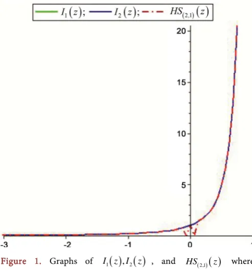
b) For a=4.2, b= −3.7, c=8.5, we have similar results, and equality of I2

( )

z

and HS( )2,1

( )

z on

(

−∞,1

)

, while I1

( )

z is not defined anywhere on

(

−∞ ∞,

)

.

Fig-ure 1 and FigFig-ure 2 illustrate the example.

[image:9.595.246.509.63.581.2]

Figure 1. Graphs of I z I1

( ) ( )

, 2 z , and HS( )2,1

( )

z where

4.2, 3.7, 6.5

a= b= c= (They coincide).

Figure 2. Graphs of I z1

( )

(a), I2

( )

z (b), and HS( )2,1

( )

z (c),

with z= +x iy, a=4.2,b=3.7,c=6.5 (They coincide).

2.3.2. Laplace Representation on the Positive Half-Line

This representation is useful when dealing with Laplace transform methods and mo-ment generating functions, which is frequent in Statistics. However, 2F1

( )

. , and later

( )

.

pFq , is usually expressed in function of another hypergeometric function, with less parameters, and this fact is useful for a progressive definition of a family of functions. We have:

(

)

_{( )}

1

(

)

2 1 1 1

0

1

, ; ; et a , ; d

F a b c z t F b c zt t

a

∞

− −

= ⋅

[image:9.595.249.496.70.336.2]

where 1F1

( )

⋅ is the confluent hypergeometric function, studied first by Kummer [22],

with single integral representation:

(

)

( )

_{( )}

_{( ) (}

( )

₎

1 1

(

)

1 1 1

0 0

, ; e 1 d

!

k

c a zt a

k k _k

a z c

F a c z t t t

c k a c a

∞ _{− −}

−

=

Γ

= = −

Γ Γ −

∑

∫

, Re

(

c−a

)

>0. (6)

or double integral representation:

( ) ( )

1 1 0 1

(

)

0 0

1

et ssa tb F ; ;c xst d ds t

a b

∞ ∞

− − − − _{⋅ −}

Γ Γ

∫ ∫

.

This hypergeometric function is an important function in its own right (see Slater [16]), but due to space limitation we will not deal with it further. On the other hand, the Laplace transform of _pF_q

( )

. is:

(

)

( )

(

)

1 1

1 1 1 1 1

0

e txt pF aq , ,a bp; , ,b tq; dt c p F aq , ,ap, ; ,b ,b xq;

x

α α _α

∞

− − −

+

Γ

= ⋅

∫

    , (see (10))

which, however, is valid only for p<q , Re

( )

α >0 , Re

( )

x >0 , or p=q ,

( )

Re α >0, and does not apply here.

MATHEMATICA gives this transform a quite complex sum of three hypergeometric functions, as follows:

(

)

{

}

( )

(

) (

_{( ) (}

) ( )

₎

(

)

(

) (

) ( )

( ) (

)

(

)

(

)(

)

(

)

( )

1

2 1 1 1

1 1 1

2 2

1

, ; ; 1, 1;

1

1,1 ;

1

1, 2 ; 2 , 2 ; , Re 0.

1 1

a

b

a b a c z

L F a b c t z F a c a b z

b c a

b a b c z

F b c a b z

a c b

c

F c a b z z

a b

−

−

Γ − Γ − Γ

− = ⋅ − + − +

Γ Γ − Γ − Γ − Γ

+ ⋅ − + − +

Γ Γ − −

+ ⋅ − − − >

− −

NOTE: Some results on this transform, and its inverse, are given on p.212 and 291 of Tables of Integral Transforms [15].

2.3.3. Mellin-Barnes Representation by Contour Integral in the Complex Plane

Complex analysis developed in the 19th century brought powerful tools such as the calculus of residues, and Mellin-Barnes formula gives a third representation, based on contour integration. The value of the integral is computed, not as a complex integral, but as the sum of the residues at poles of Γ

( )

s . When they are simple we have:

( )2,1

(

)

_{( ) ( )}

( )

(

) (

₍

₎

) ( )

( )

1

, ; ; d

2π

i

s

i

c a s b s s

HS a b c z z s

i a b c s

∞

−

− ∞

Γ Γ − Γ − Γ

= −

Γ Γ

∫

Γ − ,

(7)

Computing the residues at the simple poles of Γ

( )

s ,

{

0, 1, 2,− − 

}

, we have (4)

equal to (7) (a proof is given in 2.4.5) but for this case only. It can be shown, again, us-ing (7), that HS( )2,1

(

a b c z, ; ;

)

can be extended to a function analytic in the complex

plane, with a cut along

[ )

1,∞ .

Mathai and Saxena ([23], p. 165) gave results in the case where a and b differ by

integers and some poles become multiple. Cases b= +a m, b= +a m with

c= + +a m n, c= + +a b m, etc. were considered, and gave results distinct from the

Example 2: For a=3,b= +a 3,c=15.3, for example, we have I1

( )

z =I2

( )

z on

(

−∞,1

)

, and I₁

( )

z =I₂

( )

z =HS_{( )2,1}

( )

z on

(

−1,1

)

by direct computation, and finally,

( )2,1

( )

1

( )

2

( )

HS z =I z =I z on

(

−∞ −, 1

)

by analytic continuation, by taking as value of

( )2,1

( )

HS z the value of I₁

( )

z =I₂

( )

z within that interval. From (7) above, however,

( )2,1

(

, ; ;

)

HS a b c z is not defined for 0< <z 1 since the formula in this case contains

( )

log −z . This is a drawback from Mellin-Barnes representation.

Mellin-Barnes integral formula has its origins in the work of Pincherle in 1888 (see Mainardi and Pagnini [24]) and this formula was developed later by Mellin and Barnes. Athough (7) is very convenient to deal with when extensions of

( )2,1

(

, ; ;

)

HS a b c z to forms which are more general are considered, (7) itself is seldom

encountered in statistics.

2.3.4. Contiguous Relations

Let 2F a b c z1

(

, ; ;

)

be Gauss hypergeometric function and the associated six functions,

called contiguous functions: 2F a1

(

±1, ; ;b c z

)

, 2F a b1

(

, ±1; ;c z

)

, 2F a b c1

(

, ; ±1;z

)

. It

can be shown that 2F a b c z1

(

, ; ;

)

can be obtained as a linear combination of any two of

these functions, with rational coefficients expressed in terms of a b c, , and z. There are

hence 15 such relations, that can be generalized to 2F a1

(

+m b, +k c; +s z;

)

, with m k,

and s being integers.

2.4. Generalization to Several Parameters

2.4.1. Generalized Hypergeometric Functions

Although q+1F aq

(

1,,aq+1; ,b1,b zq;

)

is the direct generalization of Gauss

(

)

2F a b c z1 , ; ; we have, in general, the hypergeometric function in one scalar variable

and

(

p+q

)

parameters, defined as the series with expression:

( )

(

)

( )

( )

( )

( )

1

1 1

,

0 ₁

, , ; , , ;

!

n p

n n

p q

p q

n _q

n n

a a _z

HS a a b b z

n

b b

∞

=

=

∑



 

 ,

{ } { }

ai , bi ∈,z∈ (8) with Pochhammer’s notation:

( )

_{( )}

1

(

) (

)

(

) ( )

0

1

et a n 1 1

n

a t dt a a a n a n a

a

∞

− + −

= = + + − = Γ + Γ

Γ

∫

 , with

( )

a 0 =1.

(p q, )

(

1, , p; ,1 , q;

)

HS a  a b b z converges for all z when q≥ p , and diverges for 1

p> +q . For p= +q 1, it is absolutely convergent for z =1 if Re

( )

β <0,

condi-tionally convergent for z= −1 if 0≤Re

( )

β <1 and divergent for z =1 if

( )

1≤Re β . Here

1 1

p q

j j

j j

a b

β

= =

=

∑

−

∑

_.

For particular values of p and q we have the following series:

( )

0 0

0

.; e

!

k z

k z

F z

k

∞

=

=

∑

= _,

( )

( )

(

)

1 0

0

; 1

!

k

a k

k

a z

F a z z

k

∞ ₋

=

( )

_{( )}

_{( )}

( )

_{( )}

( )

_{( )}

0 1 1 2 1

0

; 2 , Bessel function

! k c c k _k c z

F c z I z I

c k z ν

∞ − − = Γ =

∑

= = _,

(

)

( )

_{( )}

(

)

1 1 0

; ; Kummer ; ; function

!

k k k _k

a z

F a c z a c z

c k

∞

=

=

∑

= Φ ,

(

)

2F a b0 , ; ;− z =Carlson s function’ ,

(

)

( ) ( )

_{( )}

2 1 , ; ; , Gauss function

!

k k k

k

a b _z

F a b c z

c k

=

∑

.

2.4.2. Analytic Continuation

Series are very useful in the resolution of differential or algebraic equations, but to study the solution’s analytic properties we rather use its integral form.

As we have seen, conditional on the values of a, b and c in 2F1

( )

. , integral (5) or (5’)

converges for any value of z, except on

[ )

1,∞ which means that the function can be

extended to any point in the complex plane, with the cut

[ )

1,∞ , provided

0, 1, 2,

c≠ − − 

For the general case, Olsson [25] proposed to express pFq as an expression of 1 1

p− Fq− progressively down to Gauss 2F1 (for p= +q 1), using (13), the analytic continuation of which has been made. For an extensive study, and lists of properties and formulas of pFq, we refer to Mathai and Saxena ([23], sect 5). As before, we have three types of integral representation:

2.4.3. Euler Integral Representation

( )

( ) (

)

(

)

( )

( )

1 1 1 1 1 1 1 1 1 0 , , , ; , , , , ,

1 ; d , Re Re 0

, ,

p p q

q

d c p

c

p q

q

a a c

F z

b b d

a a

d

t t F tz t d c

b b

c d c

+ + − − −      

Γ  

= − _{ } > >

Γ Γ −

∫

_{ }

 

 

. (9)

2.4.4. Laplace Representation on the Positive Axis

a) Laplace integral representation:

( )

0

0 1 1 1

1

1 0 0 1

, , , ₁ , ,

; e ; d

, , , ,

p t a p

p q p q

q q

a a a a a

F z t F tz t

b b a b b

∞ − − +     = ⋅

  _Γ  

 

∫

 

 

  (9’)

This relation is not to be mistaken as the Laplace transform below. b) Laplace transforms:

Considering pFq+1 and p+1Fq, using Laplace transforms, we have the couple:

( )

1 1 1 1

1

1 0 1

, , , , ,

; e ; d

, , , ,

c

p tx c p

p q p q

q q

a a c x a a

F x t F t t

b b c b b

∞

− − −

+

   

− = −

  _Γ  

 

∫

 

 

  ,

(10)

( )

1 1 1

1 1

1 1

, , , ,

; e ; d

, , , 2π , ,

p tz c p

p q c p q

q L q

a a c a a

F t z F z z

b b c t i b b

− − + − Γ     − = −      

∫

   

  , (11)

(The above expressions become Laplace and inverse Laplace transforms of _pF_q

( )

.

when c=1 and c=0 respectively. They would permit us to “circulate” between

(

p+1,q

)

,

(

p q, +1

)

, and

(

p q,

)

, under some conditions on the values of p and q.)

2.4.5. Mellin-Barnes Representation

Conversely, it can be shown that if a b_i, _j∈R are distinct of each other with differenc-es different from integers, (8) is the sum of all rdifferenc-esidudifferenc-es of Γ

( )

s . Evaluating

( )

(

)

(

)

(

)

(

)

( )( )

1 1 1 d 2π d i p s

d i q

a s a s

f z s z s

i b s b s

+ ∞

−

− ∞

Γ − Γ −

= Γ −

Γ − Γ −

∫

_ , (12)

where a bi, j are positive numbers, we have simple poles of Γ

( )

s at

, 0,1, 2,

s= −γ γ = , being negative integers. Using the formula for residue value, we

have:

( ) ( )

(

)

(

)

(

)

(

)

( )

( )

( )

( )

( )

( )

( )

1 1 1 1 1 1 1 Res ! ! p j p p j q q q j j

a _{a a}

a a _z

z

b b b b

b γ _γ γ γ γ γ γ γ λ γ

γ γ γ γ

=

=

 _Γ 

 

Γ + Γ +

−  

= − _{= } 

Γ + Γ + _{ Γ }

   

∏

∏

    . Since the poles are in infinite numbers, we can see that

( )

( )

( )

( )

( )

1

=0 0 ₁

Res

!

p q

a a _z

b b

γ

γ γ

γ γ _γ

γ γ γ ∞ ∞ = =

∑

∑

  ,

(

)

( )

( )

(

)

(

)

(

)

(

)

( )( )

1 1 1 1 1 1 1

, , ; , , ; d

2π

q

j d i

p s

j

p q p q p

d i q

j j

b

a s a s

F a a b b z s z s

i b s b s

a + ∞ − = − ∞ =

Γ _{Γ − Γ −}

= Γ −

Γ − Γ −

Γ

∏

∫

∏

  

 (13)

NOTE: We have most common functions in mathematics represented by

(

)

2F a b c z1 , ; ; where a, b and c take simple values. For example, we have:

( )

(

2

)

2 1

arctan z = F 1 2 ,1;3 2;−z . A list of standard mathematical functions expressed as

G-functions can be found in Mathai and Saxena ([23], sect. 2.6). Conversely, section 2.7 there gives G-functions expressed in terms of standard functions. Also, the software MAPLE allows us to convert a hypergeometric function into a standard function. For example, the command:

convert (hypergeom

(

[ ] [ ]

1,1 , 2 ,−x

)

, StandardFunctions);

gives as answer: ln

(

x 1

)

x

+

.

2.5. Generalization to G and H Functions

In an effort to generalize pFq

( )

⋅ and make sense of the case p> +q 1, we define the H-function, using Mellin-Barnes formula, and consider the ratio of two products of gamma functions as integrand. Fox’s H-function, is hence defined as the integral along the complex contour L, of the expression

( )

s

x

(

)

(

)

(

)

(

)

(

)

(

)

(

)

(

)

1 1 1 1

1 1 1 1

, , , , ₁ , , , ,

d 2π

, , , , , , , ,

m r

p p p p _s

p q

L

q q q q

a a a a

H x x s

i

b b b b

α α α α

ϕ

β β β β

−      ₌          

∫

 

  , (14)

where

(

)

(

)

(

)

(

)

(

) (

)

(

)

(

)

1 1 _{1 1}

1 1

1 1

1

, , , ,

, , , , ₁

m r

j j j j

p p _{j j}

q p

q q

j j j j

j m j r

b s a s

a a

b b _{b s a s}

β α

α α

ϕ

β β _{β α}

= =

= + = +

Γ + Γ − −

 

 _{ =}

  _{Γ − − Γ +}

 

∏

∏

∏

∏



 . (15)

The Meijer function G x

( )

is a special case, when αi =βj=1, ∀i j, , of H x

( )

.

We notice that (15) is just one way to generalize the integrant in (13).

From (3) and (14) we can see that G and H-functions are Inverse Mellin Transforms of ϕ

( )

. and that the Mellin-Barnes integral is now taken as the definition of the

G-function, instead of a series, or a definite integral, as in preceding sections. But under some mild conditions on a bi, j, the

( )

1 1

.

p p q

G + function can be expressed as a _pF_q

( )

.

function and conversely:

( )

( )

1

1 1 1

1

1 1

1

1 , ,1 , ,

;

0,1 , ,1 , ,

p

j p

p j p

p q p q q q q j j a

a a a a

G z F z

b b b b

b = + = Γ  − −    − = ⋅  _{− −}       

  _Γ

∏

∏

 

  . (16)

The G-function converges when L is taken as one of the two paths L∞,L−∞

encir-cling the right poles (related to aj), or the left poles (related to bj), defining G z

( )

for z <1 and z ≥1 respectively, depending on the values of p and q, or a third path

*

L can be taken as the vertical axis, separating them, for p+ <q 2

(

m+n

)

and

( )

arg z <δπ, with δ = + −m n

(

p+q

)

2, following Jordan’s lemma. For discussions

on the G-function see Mathai and Saxena [23], and on the H-function, see Springer [26], which also treats some uses of these functions in Statistics, as well as some com-putational issues. We wish to mention the following points:

1) The three paths of integration are similar to those of pFq

( )

⋅ , and the convergence of H and G now depends on

1 1 p q j j j j a b β = =

=

∑

−

∑

, and also on

1 1 j j p q j j j j α β

λ α β

= =

=

∏

∏

. 2) There are numerous properties of the Meijer G-functions: Contiguity, relations with themselves, derivatives, integral transforms, etc., that we cannot list here, due to space limitation. They can be seen in Mathai and Saxena [23].

3) The H-function can be brought to the G-function for computation, when all

,

i j

a b are positive rational numbers, by a simple change of variable and using the mul-tiplication formula for gamma functions.

4) The Euler and Laplace representations of G involve other G-functions with lesser parameters, similarly to _pF_q

( )

. ((9) and (9’)):

(

)

(

)

1

1 1 1 1 1 1

0

1 1

, , , 1 , ,

; 1 ; d

, , , , ,

m n m n

p q p p q p

q q

a a a a

G z x x G zx x

b b b b

α β α

α

β α β

+

+ +  ₌ − ₋ − − _⋅  

  _{Γ −}  

 

∫

 

 

( )

1

1 1 1 1

0

1 1

, , , , ,

; e ; d , Re 0

, , , ,

m n m n

p q p x p q p

q q

a a a a

G x y G xy y x

b b b b

α

α

+

+  − ₌ ∞ − − _⋅   _>

     

∫

      .

( )

2

2 1 2 1 2

0

1 1

0,1 2 , , , , ,

; 4 e ; d , Re 0

, , , ,

m n m n

p q p zx p q p

q q

a a a a

G z G x x z

b b η b b η

+

+  ₌ ∞ − _⋅   _>

   

 

∫

 

 

 

The Laplace transforms pair of G:

( )

1 1

1 1 1

0

1 1

, , , , ,

e ; d ; , Re 0

, , , ,

m n m n

p q p p q p

xy

q q

a a a a

y G y y x G x x

b b b b

α _η α + + α _η

∞ − − _⋅   ₌ −   _>

   

   

∫

_{ } ,

and its inverse

1 1 1 1

1 1

, , ₁ , ,

; e ; d , 0.

, , , 2π , ,

m n m n

p q p c i wx p q p

c i

q q

a a a a

x G x w G w w c

b b i b b

α _η α _η

α

+ + ∞

− −

− ∞

   

= ⋅ >

   

 

∫

 

 

 

(Taking α =0 we have the Laplace transform of

( )

.

m n p q

G ).

Also, the relation 1 1

1 1

, , 1 , ,1

; ;1

, , 1 , ,1

m n n nm

p q p q p q

q p

a a b b

G z G z

b b a a

− −     =    _{− −}       

  permits the ana-

lytic continuation of G

( )

. from inside the unit disk z ≤1 to outside it, with an

ap-propriate cut, if necessary, depending on the value of m+ −n p.

Generalizations of H-functions: We will not go beyond the H-function, but it is worth mentioning that generalized forms of H exist, e.g. the one in Rathie [27], which depends on an additional set of parameters

{

γ κ λ ζ, , ,

}

. It is defined by:

(

)

(

)

(

)

(

)

(

)

1 1 1 1 1 1 , , , ,

, , _{1 1}

d

, , 2π _{, , , ,}

m r

p q p p p s

s

p L _{q q}

a a

a a

x x s

b b i s b b

γ κ λ ξ

λ ξ

α α

ϕ

γ κ β β

− +     _{ } =   _{ } +    

∫

_{ }    _ R .

This function should not be confused with Carlson’s Rn

( )

⋅ function [10] defined in section 6.3.

But the Fox-Wright function

(

)(

)

(

)

(

)(

)

(

)

(

)

(

)

(

)

(

)

1 1 2 2 1 1

0 _{1 1}

1 1 2 2

, , ,

;

!

, , ,

j

p p p p

p q

j _{q q}

q q

a A a A a A a A j a _{A j z}

z

j

b B j b B j

b B b B b B

ψ ∞

=

  _{Γ + Γ +}

  =

  Γ + Γ +

 

∑

 

 

can be expressed as a H-function, while the MacRobert E-function, defined below, can be expressed as a G-function.

( )

( )

(

)

(

)

( )

( )

1 1 1 1 1 1 1 1 1 1 1 1 1 , , | , , , ,

| , , 0, or 1, 1

, ,

*

,1 , ,1

| 1 ,

1 , ,*, ,1

* ignor contrib ,

h p q p i p i p q q q i i p i h p q h h h q

a i

h q p q

h h p

i h i a a E x b b a a a

F x p q x p q x

b b

b

a a

a a b a b

a x F x

a a a a

b a j h − = = − = + − =      

Γ _{ }

= ⋅ _ − _ ≤ ≠ = + >

 

Γ

Γ − _{ + − + − }

⋅Γ  _{+ − + −} − 

= _{Γ −  }

= =

∏

∏

∏

∏

       1

2 or 1 & 1.

p h

p q p q x

=

≥ + ≥ + <

3. Hypergeometric Series and Functions in Several Independent

Scalar Variables

When we go from one variable to two variables there are different ways to sum the va-riables, reflected in different expressions for the coefficients given to

! !

n m

x y

n m , and

hence, we have different functions. In two variables, we have Appell hypergeometric functions, defined as follows:

3.1. Appell, Lauricella and Other Sums

(

)

( ) ( ) ( )

_{( )}

(

)

1

, 0

, , ; ; , , max , 1

! !

n m m n m n m n _{m n}

a b b x y

F a b b c x y x y

c n m

∞ +

= ₊

′

′ =

∑

< ,

(

)

( ) ( ) ( )

_{( ) ( )}

2

, 0

, , ; , ; , , 1

! !

n m m n m n m n _{m n}

a b b _{x y}

F a b b c c x y x y

c c n m

∞ +

=

′

′ ′ = + <

′

∑

,

(

)

( ) ( ) ( ) ( )

_{( )}

(

)

3

, 0

, ; , ; ; , , max , 1

! !

n m m n m n m n _{m n}

a a b b x y

F a a b b c x y x y

c n m

∞

= ₊

′ ′

′ ′ =

∑

< ,

(

)

( ) ( )

_{( ) ( )}

4

, 0

, ; , ; , , 1

! !

n m m n m n m n _{m n}

a b x y

F a b c c x y x y

c c n m

∞

+ +

=

′ = + <

′

∑

.

a) Each of these functions can be expressed as an infinite series in x alone, with coef-ficients containing Gauss function 2F1

( )

⋅,y . For example, we have:

(

)

( ) ( )

_{( )}

(

)

1 2 1

0

, , ; ; , , ; ;

!

m m m

m _m

a b x

F a b b c x y F a m b c m y

c m

∞

=

′ =

∑

⋅ + ′ + ,

and, similarly for other functions.

Also, F1

( )

⋅ and its generalization FD

( )

⋅ (see sect. 3.2), seem to be the most im-portant among these functions, with numerous applications in several disciplines.

b) Other hypergeometric functions, 34 in total, have been defined by Jacob Horn. The main ones are G1

( )

⋅ , G2

( )

⋅ , G3

( )

⋅ and H1

( )

⋅ , H2

( )

⋅ , , H7

( )

⋅ . They will

not be treated here. Whittaker, Pandey, Srivastava, Wright, Macrobert, Kampé de Fériet, and Lauricella-Saran functions, as well as lesser-known functions, will not be treated either, due to space limitation, see Exton [28].

c) Functions

Ψ

( )

⋅ and Φ ⋅

( )

of Humbert: These 7 confluent forms of the Appell series are denoted Φ1, Φ2, Φ3, Ψ1, Ψ2, Ξ1, Ξ2, and are limiting values of Ap-pell functions. For example:

[

]

( ) ( )

1

_{( )}

2

[

]

2 1 2 1 1 2

, 0

, ; ; , lim , , ; ; ,

! !

n m m n m n _{m n}

x y

x y F x y

n m α

β β

β β γ α β β γ α α

γ

∞

→∞

= ₊

Φ =

∑

= _.

They have a particular role in the representation of Appell functions. For example, we have F1

( )

⋅ as a function of Φ ⋅2

( )

. The corresponding 13 confluent forms of the

3.2. Integral Representations and Further Generalization

Lauricella functions are extensions of Appell functions to n variables, where n>2,

with FA

(

a b, ,1,b cn; ,1,c xn; 1,,xn

)

, FB

(

a1,,a bn; ,1,b c xn; ; 1,,xn

)

,

(

, ; ,1 , ; 1, ,

)

C n n

F a b c  c x  x and F_D

(

a b, ,₁,b c x_n, ; ₁,,x_n

)

corresponding,

respec-tively, to Appell functions, F a b b c c x x2

(

, ,1 2; ,1 2; 1, 2

)

, F a a b b c x x3

(

1, 2; ,1 2; ; 1, 2

)

,

(

)

4 , ; ,1 2; 1, 2

F a b c c x x and F a b b c x x₁

(

, ,_{1 2}; ; ₁, ₂

)

in 2 variables.

And the Humbert function in n variables is defined as follows:

( )

₍

₎

( )

( )

( )

1 1 1 1 1

2 1 1

, 0 1

, , ; ; , , , ! ! n n n m m n m m n n n n

m n m m n

b b _{x x}

b b c x x

c m m

∞

= _{+ +}

Φ =

∑



 _

 

 (17) 3.2.1. Integral Representation of Euler Type

These integrals represent hypergeometric functions in n variables. For example,

(

)

( )

(

)

( )

(

)

(

)

1 1 1 1 1 1 1

1 1 1

1

0 0

1

1

, , , ; ; , ,

1 n 1 d d ,

j

D n n

n

c b b a

b

j n n n

n

j n i

i

F a b b c x x

c

u u u ux ux u u

c b b b

− − − − − − = = Γ = − − − − − −

Γ − − −

∏

Γ

∫ ∫

∏



 

   



(18)

and similarly for other functions, which can serve to extend the function outside the domains of convergence of the series. The n-tuple

(

S1,,Sn

)

, where Si is either 0, 1 or ∞_{, are the regular singularities for the analytic extensions, and should be studied} separately (see Exton ([28], sect 6.7.4) for the case n=3 and F_D

( )

. ).

In particular, for F_D

( )

. , or F₁

( )

. , it can be represented by a single integral, a result

known as Picard’s Theorem 9 (although the result seemed to have been established eight years earlier). We have:

(

)

_{( ) (}

( )

₎

(

)

(

)

1

(

)

1

1 1

1 1 1

0

, , , ; ; , , a 1 c a 1 b 1 bnd

D n n n

c

F a b b c x x u u ux ux u

a c a

−

− − −

−

Γ

= − − −

Γ Γ −

∫

   . (19)

But deeper results are obtained using A-hypergeometric functions (see section 8.1.2). Also, F1

( )

⋅ has strong connections with elliptic integrals. For example, we have:

(

)

(

)

π 2 2 1 2 2 0

d π 1 1

,1, ; ,

2 2 2

1 sin 1 sin

F n k

n k θ θ θ   = _{ }   − −

∫

. (20)

Convenient forms for these integrals have been suggested by Carlson, using his own hypergeometric functions (see sect. 6.3.3).

3.2.2. Integral Representation of Laplace Type on

(

)

n

0,∞

Lauricella functions are expressed in terms of n-fold integrals of Ψ2, Φ2, 0F1 and 1F1, respectively.

Again, for FD we have a multiple integral expression:

(

)

( )

(

)

1 1

1 1 1 1 1 1 1

1 0 0

1

1

, , , ; ; , , e n j ; ; dt d

n b t t

D n n n j n n n

j i

i

F a b b c x x t F a c x t x t t

b ∞ ∞ − − − − = = = ⋅ + +

Γ

∫ ∫

∏

∏



and also a single integral representation, using Humbert function:

(

)

_{( )}

( )

₍

₎

2

1

1 1 ₀ 1 1

1

, , , ; ; , , et a n , , ; ; , , d

D n n n n

F a b b c x x t b b c x t x t t

a

∞ − −

= Φ

Γ

∫

    .

3.2.3. Representation of Mellin-Barnes Type

Integrals are taken along the infinite imaginary axis, suitably indented. For example, for

( )

D

F ⋅ we have

(

)

( )

( )

( )

( )

(

)

(

)

(

)

( ) ( )

1 1

1

1

1

1 1

1 I I

1

, , , ; ; , ,

( )

1

d d .

( )

2π

j

m m

D n n

n

n j j _{n n}

t j

j j n

n n

j j

n j

j

F a b b c x x

a t t b t

c

t x t t

c t t

i

a b

− =

= =

=

Γ − + + Γ −

Γ

= Γ −

Γ − + +

Γ Γ

∏

∏

∏

∫ ∫

∏

 



 



Analytic continuation for Appell and Lauricella series: They can be continued ana-lytically outside their convergence domain using their Euler integral representation or recurrence relations that exist between themselves. Exton ([28], sect 6.6) discusses this topic in details. In particular, the case of ( )3

( )

D

F ⋅ is carefully presented.

The presence of so many forms of hypergeometric functions in n variables is embar-rassing when we do not know the relations between them, which was the situation in the first half of the 20th century. But this situation started to change by the mid-eighties (see sect. 8.1.3).

3.3. Differential Equations and Systems

Partial and ordinary differential equations play an important role in Applied mathe-matics and to a lesser extent, in Statistics. They still constitute a major tool in the study of hypergeometric functions in pure and applied mathematics.

a) The basic hypergeometric equation (of Fuchsian type) in one variable is:

(

1

)

(

1

)

0

x −x y′′+_c− a+ +b x y_ ′−aby= , (21)

a solution of which, obtained under series form, is y1=HS( )2,1

(

a b c x, ; ;

)

. Every

second-order linear ODE with three regular singular points can be transformed into this equation. There is an extensive discussion in the literature (e.g. Lebedev [19]) on values of this solution at regular singularities 0, 1 and ∞_{, as well as when there are}

re-lations between coefficients containing integers. When c is not an integer the other

so-lution independent of the first is: 1

(

)

2 2 1 1 ,1 ; 2 ;

c

y =x− F − +c a − +c b −c x . The general

solution of (21) is hence: y=c y1 1+c y2 2, with c c1, 2 constants.

Concerning other hypergeometric functions, the equation satisfied by G-functions is:

( )

( )

1 1

d d

1 1 0

d d

p q

m n p

j k

j k

z z a z b u z

z z

+ −

= =

 ₋  _{− + −}  ₋  ₌  _ _ _ _



∏

∏

 ,

and, for partial differential systems, there is one for each Lauricella function F F FA, B, C and FD. For this last function FD, it is, for example:

(

)

2

(

)

2

(

)

2

1, 1,

1 1 1 0

n n

j j j k j j j k j

k k j k j j k k j k

j

F F F F

x x x x c a b x b x ab F

x x x x

x = ≠ = ≠

∂ ∂ _{ }∂ ∂

− + − +_ − + + _ − − =

∂ ∂ ∂ ∂