Munich Personal RePEc Archive
Scoring rules for judgment aggregation
Dietrich, Franz
CNRS (Paris, France), UEA (Norwich, U.K.)
26 December 2011
Scoring rules for judgment aggregation
Franz Dietrich1
December 2011 (minor revisions later)
Abstract
This paper studies a class of judgment aggregation rules, to be called ‘scoring rules’ after their famous counterpart in preference aggregation theory. A scoring rule delivers the collective judgments which reach the highest total ‘score’ across the individuals, subject to the judgments having to be rational. Depending on how we define ‘scores’, we obtain several (old and new) solutions to the judgment aggregation problem, such as distance-based aggregation, premise- and conclusion-distance-based aggregation, truth-tracking rules, and a Borda-type rule. Scoring rules are shown to generalize the classical scoring rules of preference aggregation theory.
JEL Classification: D70, D71
Keywords: judgment aggregation, social choice, scoring rules, Hamming rule, Borda rule, premise- and conclusion-based rules
1
Introduction
The judgment aggregation problem consists in merging many individuals’ yes/no judgments on some interconnected propositions into collective yes/no judgments on these propositions. The classical example, born in legal theory, is that three jurors in a court trial disagree on which of the following three propositions are true: the defendant has broken the contract (p); the contract is legally valid (q); the defendant is liable (r). According to a univer-sally accepted legal doctrine, r (the ‘conclusion’) is true if and only if p and r (the two ‘premises’) are both true. So, r is logically equivalent to p∧q. The simplest rule to ag-gregate the jurors’ judgments — namely propositionwise majority voting — may generate logically inconsistent collective judgments, as Table 1 illustrates. There are of course
nu-premisep premiseq conclusionr(⇔p∧q)
Individual 1 Yes Yes Yes
Individual 2 Yes No No
Individual 3 No Yes No
Majority Yes Yes No
Table 1: The classical example of logically inconsistent majority judgments
merous other possible ‘agendas’, i.e., kinds of interconnected propositions a group might face. Preference aggregation is a special case with propositions of the form ‘xis better than
1CNRS, Cerses, Paris, France & UEA, Norwich, U.K. Mail: [email protected]. Web:
y’ (for many alternatives x and y), where these propositions are interconnected through standard conditions such as transitivity. In this context, Condorcet’s classicalvoting para-dox about cyclical majority preferences is nothing but another example of inconsistent majority judgments. Starting with List and Pettit’s (2002) seminal paper, a whole series of contributions have explored which judgment aggregation rules can be used, depending on, firstly, the agenda in question, and, secondly, the requirements placed on aggregation, such as anonymity, and of course the consistency of collective judgments. Some theorems generalize Arrow’s Theorem from preference to judgment aggregation (Dietrich and List 2007, Dokow and Holzman 2010; both build on Nehring and Puppe 2010a and strengthen Wilson 1975). Other theorems have no immediate counterparts in classical social choice theory (e.g., List 2004, Dietrich 2006a, 2010, Nehring and Puppe 2010b, Dietrich and Mongin 2010).
It is fair to say that judgment aggregation theory has until recently been dominated by ‘impossibility’ findings, as is evident from theSymposium on Judgment Aggregation in Journal of Economic Theory (C. List and B. Polak eds., 2010, vol. 145(2)). The recent conference ‘Judgment aggregation and voting’ (Freudenstadt, 2011) however marks a visible shift of attention towards constructing concrete aggregation rules and finding ‘second best’ solutions in the face of impossibility results. The new proposals range from a first Borda-type aggregation rule (Zwicker 2011) to, among others, new distance-based rules (Duddy and Piggins 2011) and rules which approximate the majority judgments when these are inconsistent (Nehring, Pivato and Puppe 2011). The more traditional proposals include premise- and conclusion-based rules (e.g., Kornhauser and Sager 1986, Pettit 2001, List & Pettit 2002, Dietrich 2006, Dietrich and Mongin 2010), sequential rules (e.g., List 2004, Dietrich and List 2007b), distance-based rules (e.g., Konieszni and Pino-Perez 2002, Pigozzi 2006, Miller and Osherson 2008, Eckert and Klamler 2009), and quota rules with well-calibrated acceptance thresholds and varous degrees of collective rationality (e.g., Dietrich and List 2007b; see also Nehring and Puppe 2010a).
The present paper contributes to the theory’s current ‘constructive’ effort by investi-gating a class of aggregation rules to be calledscoring rules. The inspiration comes from classical scoring rules in preference aggregation theory. These rules generate collective pref-erences which rank each alternative according to the sum-total ‘score’ it receives from the group members, where the ‘score’ could be defined in different ways, leading to different classical scoring rules such as Borda rule (see Smith 1973, Young 1975, and for abstract generalizations Myerson 1995, Zwicker 2008 and Pivato 2011b). In a general judgment aggregation framework, however, there are no ‘alternatives’; so our scoring rules are based on assigning scores to propositions, not alternatives. Nonetheless, our scoring rules are related to classical scoring rules, and generalize them, as will be shown.
scoring, to be called reversal scoring, will lead to a new generalization of Borda rule from preference aggregation to judgment aggregation. The problem of how to generalize Borda rule has been a long-lasting open question in judgment aggregation theory. Recently, an interesting, though so far incomplete, proposal was made by Zwicker (2011) (who told me that also Conal Duddy and Ashley Piggins have independent work in progress about this). Surprisingly, Zwicker’s and the present Borda generalizations are distinctively different.
Though large, the class of scoring rules is far from universal: some important aggrega-tion rules fall outside this class (notably the menaggrega-tioned rule approximating the majority judgments, by Nehring, Pivato and Puppe 2011). I will also investigate a natural general-ization of scoring rules, to be calledset scoring rules, which are based on assigning scores to entire judgment sets rather than single propositions (judgments). Set scoring rules are for instance interesting in the context of epistemic (‘truth-tracking’) aggregation models, where they have recently been studied by Pivato (2011a).
I could have written this paper by focusing exclusively on one specific application of scoring rules (for instance, the problem of extending Borda rule). However, I chose to give the paper a broader scope, not only to do justice to the diverse applications of scoring rules, but also to be useful at the theory’s current stage of searching for concrete mechanisms. I hope that the ideas and perspectives offered below will be stimulating and inspiring.
After this introduction, Section 2 defines the general framework, Section 3 analyses various scoring rules, Section 4 goes on to analyse several set scoring rules, and Section 5 draws some conclusions about where we stand in terms of concrete aggregation procedures.
2
Agenda, aggregation rules, and examples
I now introduce the framework, following List and Pettit (2002) and Dietrich (2007).2 We
consider a set ofn(≥2) individuals, denotedN ={1, ..., n}. They need to decide which of certain interconnected propositions to ‘believe’ or ‘accept’. The set of propositions under consideration — the agenda — is closed under negation, which ensures that whenever, say, ‘it rains’ is a candidate for belief, so is ‘it does not rain’. The agenda is thus a (disjoint) union of binary ‘issues’ {p,¬p}involving a proposition and its negation. Rationally, ex-actly one proposition from each issue is accepted, and this in accordance with the logical interconnections. Formally, the agenda is simply an arbitrary set X (whose elements we call ‘propositions’) which is
• closed under negation: for every propositionpinX there is a specified proposition denoted¬p(‘notp’) inX such that¬p=p=¬¬p(i.e., such thatX is partitioned into binary issues{p,¬p});
• endowed with logical interconnections: there is a specification of which subsets ofX
are ‘consistent’, i.e., formally, there is a systemC of subsets called ‘consistent’. A ‘judgment set’ A⊆ X is complete if it contains a member of each pair p,¬p∈ X, and (fully) rational if it is complete and consistent. The set of all rational judgment sets is denote byD.3
2To be precise, I use a slimmer variant of their models: I do not explicitly introduce the logicLin which
propositions are formed.
3Our notion of an ‘agenda’ is very general. The propositions inXtypically represent what an agent
As usual in the theory, we assume that the consistency notion is regular. Regularity can be expressed by three conditions: no set{p,¬p}is consistent (C1, ‘self-entailment’); subsets of consistent sets are consistent (C2, ‘monotonicity’); ∅is consistent and each consistent set can be extended to a complete and consistent set (C3, ‘completability’). Equivalently, regularity can be expressed by a single condition: C = {C ⊆ A : A ∈ D} = ∅, i.e., the consistent sets are precisely the subsets of rational sets. The systems D and C are thus interdefinable, so that, given regularity, we could start from D instead of C as the primitive.4
Further, let X be finite. Notationally, a judgment set A ⊆ X is often abbreviated by concatenating its members in any order (so, p¬q¬r is short for {p,¬q,¬r}); and the negation-closure of a setY ⊆Xis denoted
Y± ≡ {p,¬p:p∈Y}.
I now give two standard examples, to which I shall repeatedly refer.
Example 1: the standard ‘doctrinal paradox agenda’. The agenda is
X={p, q, r}±.
Logical interconnections are defined relative to the external constraint r↔(p∧q). So,
D={pqr, p¬q¬r,¬pq¬r,¬p¬q¬r}.
Example 2: the preference agenda. For an arbitrary, finite set of alternatives K, the
preference agenda is defined as
X=XK={xP y:x, y∈K, x=y},
where the negation of a proposition xP y is of course ¬xP y = yP x, and where logical interconnections are defined relative to the usual conditions of transitivity, asymmetry and connectedness, which define astrict linear order. Formally, to each binary relation≻over
K uniquely corresponds a judgment set, denotedA≻={xP y∈X:x≻y}, and the set of
all rational judgment sets is
D={A≻: ≻ is a strict linear order overK}.
A (multi-valued) aggregation rule is a correspondence F which to every profile of ‘individual’ judgment sets (A1, ..., An) (from some domain, usually Dn) assigns a set
sets’). The propositions could be thought of for instance as being syntactic objects (logical expressions) or semantic objects (e.g., sets of worlds). It is often natural to regard the agendaXas a subset of a logic Lfrom which it inherits the negation operator and the logical interconnections. This logic is general: it could for instance be standard propositional logic, standard predicate logic, or various modal or conditional logics (see Dietrich 2007).
4Instead of starting from the system of consistent setsCsatisfying C1-C3 and deriving the systemDof
rational judgment sets, we could equivalently have started fromD(any non-empty system of sets containing exactly one member from each pair p,¬p∈X) and derived the system C:=∪A∈D{C :C ⊆A}(which
F(A1, ..., An) of ‘collective’ judgment sets. Typically, the output F(A1, ..., An) is a
sin-gleton set {C}, in which case we identify this set withC and writeF(A1, ..., An) =C. If
F(A1, ..., An)contains more than one judgment set, there is a ‘tie’ between these judgment
sets. An aggregation rule is called single-valued or tie-free if it always generates a single judgment set. A standard (single-valued) aggregation rule ismajority rule; it is given by
F(A1, ..., An) ={p∈X:p∈Ai for more than half of the individualsi}
and generates inconsistent collective judgment sets for many agendas and profiles. If both individual and collective judgment sets are rational (i.e., inD), the aggregation rule defines a correspondencesDn⇒D, and in the case of single-valuedness a functionDn→ D.5
3
Scoring rules
Scoring rules are particular judgment aggregation rules, defined on the basis of a so-called scoring function. A scoring function — or simply ascoring — is a functions:X× D →R
which to each proposition pand rational judgment set A assigns a numbersA(p), called
the score of p given A and measuring how p performs (‘scores’) from the perspective of holding judgment setA. As an elementary example, so-calledsimple scoring is given by:
sA(p) =
1 ifp∈A
0 ifp∈A, (1)
so that all accepted propositions score 1, whereas all rejected propositions score 0. This and many other scorings will be analysed. Let us think of the score of asetof propositions as the sum of the scores of its members. So, the scoringsis extended to a function which (given the agent’s judgment setA∈ D) assigns to each set C⊆X the score
sA(C)≡ p∈C
sA(p).
A scoringsgives rise to an aggregation rule, called thescoring rule w.r.t. sand denoted
Fs. Given a profile (A1, ..., An) ∈ Dn, this rule determines the collective judgments by
selecting the rational judgment set(s) with the highest sum-total score across all judgments and all individuals:
Fs(A1, ..., An) = judgment set(s) inDwith highest total score
= argmaxC∈D
p∈C,i∈N
sAi(p) = argmaxC∈D
i∈N
sAi(C).
By a scoring rule simpliciter we of course mean an aggregation rule which is a scoring rule w.r.t. some scoring. Different scorings s and s′ can generate the same scoring rule Fs=Fs′, in which case they are calledequivalent. For instance,sis equivalent tos′= 2s.6
5More generally, dropping the requirement of collective rationality, we have a correspondenceDn⇒2X,
where2Xis the set ofalljudgment sets, rational or not. As usual, I write ‘⇒’ instead of ‘→’ to indicate
amulti-function.
6More generally, certain increasing transformations have no effect. As one may show, scoringssands′
are equivalent (i.e.,Fs=Fs′) whenever there are coefficientsa >0andbp∈R(p∈X) withbp=b¬pfor
allp∈Xsuch thats′
is given bys′
3.1
Simple scoring and the Hamming rule
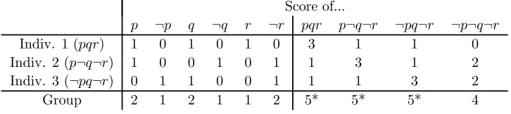
We first consider the most elementary definition of scoring, namely simple scoring (1). Table 2 illustrates the corresponding scoring ruleFsfor the case of the agenda and profile
of our doctrinal paradox example. The entries in Table 2 are derived as follows. First, enter
Score of...
p ¬p q ¬q r ¬r pqr p¬q¬r ¬pq¬r ¬p¬q¬r
Indiv. 1 (pqr) 1 0 1 0 1 0 3 1 1 0 Indiv. 2 (p¬q¬r) 1 0 0 1 0 1 1 3 1 2 Indiv. 3 (¬pq¬r) 0 1 1 0 0 1 1 1 3 2
[image:7.595.115.478.153.234.2]Group 2 1 2 1 1 2 5* 5* 5* 4
Table 2: Simple scoring (1) for the doctrinal paradox agenda and profile
the score of each proposition (p,¬p, q, ...) from each individual (1, 2 and 3). Second, enter each individual’s score of each judgment set by taking the row-wise sum. For instance, individual 1’s score ofpqris1 + 1 + 1 = 3, and his score of p¬q¬ris1 + 0 + 0 = 1. Third, enter the group’s score of each proposition by taking the column-wise sum. For instance, the group’s score of pis1 + 1 + 0 = 2. Finally, enter the group’s score of each judgment set, by taking either a vertical or a horizontal sum (the two give the same result), and add a star ‘*’ in the field(s) with maximal score to indicate the winning judgment set(s). For instance, the group’s score of pqr using a vertical sum is 3 + 1 + 1 = 5, and using a horizontal sum it is2 + 2 + 1 = 5. Since the judgment setspqr,p¬q¬rand¬pq¬rall have maximal group score, the scoring rule delivers a tie:
F(A1, A2, A3) ={pqr, p¬q¬r,¬pq¬r}.
This is a tie between the premise-based outcome pqr and the conclusion-based outcomes
p¬q¬rand¬pq¬r. Were we to add more individuals, the tie would presumably be broken in one way or the other. In large groups, ties are a rare coincidence.
To link simple scoring to distance-based aggregation, suppose we measure the distance between two rational judgment sets by using some distance function (‘metric’)doverD.7
The most common example is Hamming distance d=dHam, defined as follows (where by
a ‘judgment reversal’ I mean the replacement of an accepted proposition by its negation):
dHam(A, B) = number of judgment reversals needed to transformA intoB
= |A\B|=|B\A|= 1
2|A△B|.
For instance, the Hamming-distance between pqr and p¬q¬r (for our doctrinal paradox agenda) is 2.
Now the distance-based rule w.r.t. distance d is the aggregation rule Fd which for
any profile (A1, ..., An)∈ Dn determines the collective judgment set(s) by minimizing the
sum-total distance to the individual judgment sets:
Fd(A1, ..., An) = judgment set(s) inDwith minimal sum-distance to the profile
= argminC∈D
i∈N
d(C, Ai).
7A distance function ormetric overDis a function d:D × D →[0,∞)satisfying three conditions: for all A, B, C∈ D, (i)d(A, B) = 0⇔A=B, (ii) d(A, B) =d(B, A)(‘symmetry’), and (iii)d(A, C)≤
The most popular example, Hamming ruleFdH a m, can be characterized as a scoring rule:
Proposition 1 The simple scoring rule is the Hamming rule.
3.2
Classical scoring rules for preference aggregation
I now show that our scoring rules generalize the classical scoring rules of preference ag-gregation theory. Consider the preference agenda X for a given set of alternatives K of finite size k. Classical scoring rules (such as Borda rule) are defined by assigning scores to alternatives inK, not to propositionsxP yinX. Given a strict linear order≻overK, each alternativex∈K is assigned a scoreSCO≻(x)∈R. The most popular example is of
course Borda scoring, for which the highest ranked alternative in K scoresk, the second-highest k−1, the third-highest k−2, ..., and the lowest 1. Given a profile (≻1, ...,≻n)
of individual preferences (strict linear orders), the collective ranks the alternatives x∈X
according to their sum-total score i∈NSCO≻i(x). To translate this into the judgment
aggregation formalism, recall that each strict linear order ≻over K uniquely corresponds to a rational judgment set A∈ D (given by xP y∈A ⇔x≻y); we may therefore write
SCOA(x)instead of SCO≻(x), and view the classical scoringSCO as a function of(x, A)
inK×D. Formally, I define aclassical scoring as an arbitrary functionSCO:K×D →R, and theclassical scoring rule w.r.t. it as the judgment aggregation ruleF≡FSCO for the
preference agenda which for every profile (A1, ..., An)∈ Dn returns the rational judgment
set(s) that rank an alternative xover another y wheneverxhas a higher sum-total score thany:8
F(A1, ..., An) ={C∈ D:C contains allxP y∈Xs.t. i∈N
SCOAi(x)>
i∈N
SCOAi(y)}.
Now, any given classical scoringSCOinduces a scoringsin our (proposition-based) sense. In fact, there are two canonical (and, as we will see, equivalent) ways to defines: one might define seither by
sA(xP y) =SCOA(x)−SCOA(y), (2)
or, if one would like the lowest achievable score to be zero, by
sA(xP y) = max{SCOA(x)−SCOA(y),0}=
SCOA(x)−SCOA(y) ifxP y∈A
0 ifxP y∈A
(3) (where the last equality assumes that SCOA(x) > SCOA(y) ⇔ xP y ∈ A for all x, y
and A, a property that is so natural that we might have built it into the definition of a ‘classical scoring’ SCO). This allows us to characterize classical scoring rules in terms of proposition-based rather than alternative-based scoring:
8A technical difference between the standard notion of a scoring rule in preference aggregation theory
and our judgment-theoretic rendition of it arises when there happen to exist distinct alternatives with identical sum-total score. In such cases, the standard scoring rule returns collectiveindifferences, whereas ourFSCOreturns atiebetweenstrictpreferences. From a formal perspective, however, the two definitions
Proposition 2 In the case of the preference agenda (for any finite set of alternatives), every classical scoring rule is a scoring rule, namely one with respect to a scoringsderived from the classical scoring SCO via (2) or via (3).
3.3
Reversal scoring and a Borda rule for judgment aggregation
Given the agent’s judgment set A, let us think of the score of a proposition p ∈X as a measure of how ‘distant’ the negation¬pis fromA; so,pscores high if¬pis far fromA, and low if¬pis contained inA. More precisely, let the score of a propositionpgivenA∈ Dbe the number of judgment reversals needed to rejectp, i.e., the number of propositions inA
that must (minimally) be negated in order to obtain a consistent judgment set containing
¬p. So, denoting the judgment set arising fromAby negating the propositions in a subset
R⊆AbyA¬R= (A\R)∪ {¬r:r∈R}, so-calledreversal scoring is defined by
sA(p) = number of judgment reversals needed to rejectp (4)
= min
R⊆A:A¬R∈D&p∈A¬R|
R|= min
A′∈D:p∈A′|A\A
′|= min
A′∈D:p∈A′dHam(A, A ′).
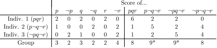
For instance, a rejected proposition p∈A scores zero, sinceA itself contains ¬pso that it suffices to negate zero propositions (R = ∅). An accepted proposition p ∈ A scores 1 if A remains consistent by negating p (R = {p}), and scores more than 1 otherwise (R {p}). Table 3 illustrates reversal scoring for our doctrinal paradox example. For instance, individual 1’s judgment set pqr leads to a score of 2 for proposition p, since in order for him to reject phe needs to negate not justp(as¬pqr is inconsistent), but also
r (where ¬pq¬ris consistent). The scoring rule delivers a tie between the judgment sets
Score of...
p ¬p q ¬q r ¬r pqr p¬q¬r ¬pq¬r ¬p¬q¬r
Indiv. 1 (pqr) 2 0 2 0 2 0 6 2 2 0 Indiv. 2 (p¬q¬r) 1 0 0 2 0 2 1 5 2 4 Indiv. 3 (¬pq¬r) 0 2 1 0 0 2 1 2 5 4
[image:9.595.116.477.411.491.2]Group 3 2 3 2 2 4 8 9* 9* 8
Table 3: Reversal scoring (4) for the doctrinal paradox agenda and profile
p¬q¬rand¬pq¬r. This is a tie between two conclusion-based outcomes; the premise-based outcomepqris rejected (unlike for simple scoring in Section 3.1).
The remarkable feature of reversal scoring rule is that it generalizes Borda rule from preference to judgment aggregation. Borda rule is initially only defined for the preference agendaX (for a given finite set of alternatives), namely as the classical scoring rule w.r.t. Borda scoring; see the last subsection. The key observation is that reversal scoring is intimately linked to Borda scoring:
Remark 1 In the case of the preference agenda (for any finite set of alternatives), reversal scoring sis given by (3) withSCO defined as classical Borda scoring.
¬xP y=yP x∈A, which impliessA(xP y) = 0, as required by (3). Now supposexP y∈A.
Clearly,SCOA(x)> SCOA(y). Consider the alternatives in the order≻established byA:
xk ≻xk−1≻ · · · ≻x≻ · · · ≻y≻ · · · ≻x1,
where xj is the alternative withSCOA(xj) =j. Step by step, we now movey up in the
ranking, where each step consists in raising the position (score) of y by one. Each step corresponds to negating one proposition in A, namely the propositionzP ywhere zis the alternative that is currently being ‘overtaken’ by y. After exactly SCOA(x)−SCOA(y)
steps,yhas ‘overtaken’x, i.e.,xP yhas been negated. So,sA(xP y)isat most SCOA(x)−
SCOA(y). It isexactly SCOA(x)−SCOA(y), since, as the reader may check, no smaller
number of judgment reversals allows yto ‘overtake’xin the ranking.
Remark 1 and Proposition 2 imply that reversal scoring allows us to extend Borda rule to arbitrary judgment aggregation problems:
Proposition 3 The reversal scoring rule generalizes Borda rule, i.e., matches it in the case of the preference agenda (for any finite set of alternatives).
I note that one could use a perfectly equivalent variant of reversal scorings which, in the case of the preference agenda, is related to classical Borda scoringSCOvia (2) instead of (3):
Remark 2 Reversal scorings is equivalent (in terms of the resulting scoring rule) to the scoring s′ given by
s′A(p) =sA(p)−sA(¬p) =
sA(p) if p∈A −sA(¬p) if p∈A,
and in the case of the preference agenda (for any finite set of alternatives) this scoring is given by
s′A(xP y) =SCOA(x)−SCOA(y)
with SCO defined as classical Borda scoring.
For comparison, I now sketch Zwicker’s (2011) interesting approach to extending Borda rule to judgment aggregation — let me call such an extension a ‘Borda-Zwicker’ rule. The motivation derives from a geometric characterization of Borda preference aggregation ob-tained by Zwicker (1991). Let me write the agenda as X={p1,¬p1, p2,¬p2, ..., pm,¬pm},
wheremis the number of ‘issues’. Each profile gives rise to a vectorv≡(v1, ..., vm)inRm
whosejthentryv
j is thenet support for pj, i.e., the number of individuals acceptingpj
mi-nus the same number for¬pj. Now ifXis the preference agenda for any finite set of
alterna-tivesK, then eachpjtakes the formxP yfor certain alternativesx, y∈K. Each preference
cycle can be mapped to a vector inRm; for instance, ifp1=xP y,p2=yP zandp3=xP z,
then the cycle x ≻ y ≻ z ≻ x becomes the vector (1,1,−1,0, ...,0) ∈ Rm. The linear span of all vectors corresponding to preference cycles defines the so-called ‘cycle space’
Vcycle ⊆Rm, and its orthogonal complement defines the ‘cocycle space’ Vcocycle ⊆Rm.
Let vcocycle be the orthogonal projection of v on the cocycle space Vcocycle. Intuitively, vcocyclecontains the ‘consistent’ or ‘acyclic’ part ofv. The upshot is that the Borda
above (below) yif the jth entry ofvcocyleis positive (negative). Zwicker’s strategy for
ex-tending Borda rule to judgment aggregation is to define a subspaceVcycle analogously for
agendas other than the preference agenda; one can then again projectvon the orthogonal
complement ofVcycleand determine collective ‘Borda’ judgments according to the signs of
the entries of this projection. This approach has proved successful for simple agendas, in which there is a natural way to defineVcycle. Whether the approach is viable for general
agendas (i.e., whetherVcycle has a useful general definition) seems to be open so far.9
A Borda-Zwicker rule is not just constructed differently from a scoring rule in our sense, but, as I conjecture, it also cannot generally be remodelled as a scoring rule, since most interesting scoring rules use information that goes beyond the information contained in the profile’s ‘net support vector’ v ∈Rm. (Even more does the required information go
beyond the projection ofvon the orthogonal complement ofVcycle.)
In summary, there seem to exist two quite different approaches to generalizing Borda aggregation. One approach, taken by Zwicker, seeks to filter out the profile’s ‘inconsistent component’ along the lines of the just-described geometric technique. The other approach, taken here, seeks to retain the principle of score-maximization inherent in Borda aggrega-tion (with scoring now defined at the level of proposiaggrega-tions, not alternatives, as these do not exist outside the world of preferences). The normative core of the scoring approach is to use information about someone’s strength of accepting a proposition (as measured by the score), just as Borda preference aggregation uses information about someone’sstrength
of preferring one alternative xover another y (as measured by the score of xP y, i.e., the difference between x’s and y’s score). Whether strength or intensity of preference is a permissible or even meaningful concept is a notoriously controversial question; the purely ordinalist approach takes a sceptical stance here. This is where Borda preference aggrega-tion differs from Condorcet’s rule of pairwise majority voting, which uses only the (ordinal) information of whether someone prefers an alternative over another, without attempting to extract strength-of-preference information from that person’s full preference relation.
3.4
A generalization of reversal scoring
Recall that the reversal score of a proposition pcan be characterized as the distance by which one must deviate from the current judgment set in order to rejectp— where ‘distance’ is understood as Hamming-distance. It is natural to also consider other kinds of a distance. Relative to any given distance functiondover D, one may define a corresponding scoring by
sA(p) = distance by which one must depart fromA to rejectp (5)
= min
A′∈D:p∈A′d(A, A ′).
This provides us with a whole class of scoring rules, all of which are variants of our judgment-theoretic Borda rule. In the special case of the preference agenda, we thus obtain new variants of classical Borda rule.
Interestingly, if we adopt Duddy and Piggins’ (2011) distance function, i.e., ifd(A, A′)
is the number of minimal consistent modifications needed to transformA intoA′,10 then
9One might at first be tempted to generally define Vcycle as the linear span of those vectors which correspond to the agenda’sminimal inconsistent subsets. Unfortunately, this span is often the entire space
Rm, an example for this being our doctrinal paradox agenda.
scoring (5) reduces to simple scoring (1), and so the scoring rule reduces to the Hamming rule by Proposition 1. So, ironically, while Duddy and Piggins had introduced their distance in the different context of distance-based aggregation to develop an alternative to Hamming rule, when we use their distance (instead of Hamming’s) in our context of scoring rules we are led back to Hamming rule.
3.5
Scoring based on logical entrenchment
We now consider scoring rules which explicitly exploit the logical structure of the agenda. Let us think of the score of a proposition p(∈X) given the judgment setA (∈ D) as the degree to whichpis logically entrenched in the belief systemA, i.e., as the ‘strength’ with whichAentailsp. We measure this strength by the number of ways in whichpis entailed by A, where each ‘way’ is given by a particular judgment subset S ⊆A which entails p, i.e., for which S∪ {¬p}is inconsistent. IfAdoes not contain p, then no judgment subset — not even the full set A— can entailp; so the strength of entailment (score) ofpis zero. If A containsp, then pis entailed by the judgment subset{p}, and perhaps also by very different judgment subsets; so the strength of entailment (score) of pis positive and more or less high.
There are different ways to formalise this idea, depending on precisely which of the judgment subsets that entail p are deemed relevant. I now propose four formalizations. Two of them will once again allow us to generalize Borda rule from preference to judgment aggregation. These generalizations differ from that based on reversal scoring in Section 3.3.
Our first, naive approach is to counteachjudgment subset which entailspas a separate, full-fledged ‘way’ in whichpis entailed. This leads to so-calledentailment scoring, defined by:
sA(p) = number of judgment subsets which entail p (6)
= |{S⊆A:S entailsp}|.
Ifp∈AthensA(p) = 0, while ifp∈AthensA(p)≥2|X|/2−1sincepis entailed by at least
all setsS ⊆Awhich containp, i.e., by at least2|A|−1 = 2|X|/2−1 sets. One might object
that this definition of scoring involves redundancies, i.e., ‘multiple counting’. Suppose for instancepbelongs toAand is logically independent of all other propositions inA. Thenp
is entailed by several subsetsSofA— allS⊆Awhich containp— and yet these entailments are essentially identical since all premises in S other thanpare irrelevant.
I now present three refinements of scoring (6), each of which responds differently to the mentioned redundancy objection. In the first refinement, we count two entailments of p
as different only if they have no premise in common. This leads to what I call disjoint-entailment scoring, formally defined by:
sA(p) = number ofmutually disjoint judgment subsets entailingp (7)
= max{m:Ahasm mutually disjoint subsets each entailingp}.
In the mentioned case where p(∈A) is logically independent of all other propositions in
A, we now avoid ‘multiple counting’: sA(p)is only 1, as one cannot find different mutually
disjoint judgment subsets entailing p. For our doctrinal paradox agenda and profile, the scoring rule delivers a tie between the two conclusion-based outcomes p¬q¬r and¬pq¬r,
Score of...
p ¬p q ¬q r ¬r pqr p¬q¬r ¬pq¬r ¬p¬q¬r
Indiv. 1 (pqr) 2 0 2 0 2 0 6 2 2 0 Indiv. 2 (p¬q¬r) 1 0 0 2 0 2 1 5 2 4 Indiv. 3 (¬pq¬r) 0 2 1 0 0 2 1 2 5 4
[image:13.595.115.476.145.223.2]Group 3 2 3 2 2 4 8 9* 9* 8
Table 4: Disjoint-entailment scoring (7) for the doctrinal paradox agenda and profile
as illustrated in Table 4. For instance, individual 2 has judgment set p¬q¬r, so that p
sores 1 (it is entailed by {p} but by no other disjoint judgment subset), ¬q scores 2 (it is disjointly entailed by {¬q}and {p,¬r}), ¬r scores 2 (it is disjointly entailed by {¬r}
and{¬q}), and all rejected propositions score zero (they are not entailed by any judgment subsets).
Disjoint-entailment scoring turns out to match reversal scoring for our doctrinal paradox agenda (check that Tables 3 and 4 coincide), as well as for the preference agenda (as shown later). Is this pure coincidence? The general relationship is that the disjoint-entailment score of a propositionpis alwaysat most the reversal score, as one may show.11
While this refinement of naive entailment scoring (6) avoids ‘multiple counting’ by only counting entailments with mutually disjoint sets of premises, the next two refinements use a different strategy to avoid ‘multiple counting’. The new strategy is to count only those entailments whose sets of premises areminimal— with minimality understood either in the sense that no premises can be removed, or in the sense that no premises can be logically weakened. To begin with the first sense of minimality, I say that a set minimally entails p(∈X) if it entailspbut no strict subset of it entailsp, and I define minimal-entailment scoring by
sA(p) = number of judgment subsets which minimally entailp (8)
= |{S⊆A:S minimally entailsp}|.
If for instance pis contained inA, then{p}minimally entailsp,12 but strict supersets of
{p}do not and are therefore not counted. For our doctrinal paradox agenda, this scoring happens to coincide with reversal scoring and disjoint-entailment scoring. Indeed, Table 3 resp. 4 still applies; e.g., for individual 2 with judgment set p¬q¬r, pstill scores 1 (it is minimally entailed only by {p}),¬qstill scores 2 (it is minimally entailed by{¬q}and by
{p,¬r}),¬rstill scores 2 (it is minimally entailed by{¬r}and by{¬q}), and all rejected propositions still score zero (they are not minimally entailed by any judgment subsets).
Scoring (8) is certainly appealing. Nonetheless, one might complain that it still al-lows for certain redundancies, albeit of a different kind. Consider the preference agenda with set of alternatives K = {x, y, z, w}, and the judgment set A = {xP y, yP z, zP w, 1 1The reason is that, givenmmutually disjoint judgment subsets which each entailp, the reversal score
of p is at least msince one must negate at least one proposition from each of these msets in order to consistently rejectp.
xP z, yP w, xP w} (∈ D). The proposition xP w is minimally entailed by the subset
S ={xP y, yP z, zP w}. While this entailment is minimal in the (set-theoretic) sense that we cannot remove premises, it is non-minimal in the (logical) sense that we can weaken
some of its premises: if we replace xP y and yP z in S by their logical implicationxP z, then we obtain a weaker set of premises S′ = {xP z, zP w} which still entails xP w. We
shall say that S fails to ‘irreducibly’ entail xP w, in spite of minimally entailing it. In general, a set of propositions is calledweaker than another one (which is calledstronger) if the second set entails each member of the first set, but not vice versa. A set S (⊆X) is defined toirreducibly(orlogically minimally) entailpifS entailsp, and moreover there is no subset Y S which can be weakened (i.e., for which there is a weaker set Y′ ⊆X
such that(S\Y)∪Y′ still entailsp). Each irreducible entailment is a minimal entailment,
as is seen by taking Y′ =∅.13 In the previous example, the set {xP y, yP z, zP w}
mini-mally, but not irreducibly entails xP w, and the set {xP z, zP w}irreducibly entailsxP w.
Irreducible-entailment scoring is naturally defined by
sA(p) = number of judgment subsets whichirreducibly entailp (9)
= |{S⊆A:S irreducibly entails p}|.
This scoring matches reversal scoring and both previous scorings in the case of our doc-trinal paradox example: Table 3 resp. 4 still applies. But for many other agendas these scorings all deviate from one another, resulting in different collective judgments. As for the preference agenda, we have already announced the following result:
Proposition 4 Disjoint-entailment scoring (7) and irreducible-entailment scoring (9) match reversal scoring (4) in the case of the preference agenda (for any finite set of alternatives).
Propositions 3 and 4 jointly have an immediate corollary.
Corollary 1 The scoring rules w.r.t. scorings (7) and (9) both generalize Borda rule, i.e., match it in the case of the preference agenda (for any finite set of alternatives).
3.6
Propositionwise scoring and a way to repair quota rules with
non-rational outputs
We now consider a special class of scorings: propositionwise scorings. This will allow us to relate scoring rules to the well-known judgment aggregation rules called quota rules — in fact, to ‘repair’ these rules by rendering their outcomes rational across all profiles.
I call scoring s propositionwise if the score of a proposition p ∈ X only depends on whether pis accepted, i.e., if sA(p) =sB(p)wheneverA and B (in D) both containpor
both do not containp. Equivalently, scoring is propositionwise just in case for eachp∈X
there is a pair of real numberss+(p), s−(p)such that
sA(p) = s+(p) for allA∈ Dcontainingp
s−(p) for allA∈ Dnot containingp.
(10)
Intuitively, s+(p) is the score of an accepted proposition p, and s−(p) is the score of a
rejected propositionp. Typically, of course,s+(p)> s−(p). An example is simple scoring:
there, s+(p) = 1ands−(p) = 0.
How do propositionwise scoring rules behave? They derive a propositionp’s sum-total score ‘locally’, i.e., based only on people’s judgments about p. This property stands in obvious analogy to a well-studied axiom on aggregation rules, namely the axiom of propo-sitionwiseorindependentaggregation, which prescribes that the collective judgment about any given proposition p is derived ‘locally’, i.e., again based only on people’s judgments about p. Can we therefore relate propositionwise scoring to independent aggregation? The paradigmatic independent aggregation rules are the quota rules.14 A quota rule is a
(single-valued) aggregation rule which is given by an acceptance threshold mp∈ {1, ..., n}
for each propositionp∈X. The quota rule corresponding to the so-calledthreshold family
(mp)p∈X is denotedF(mp)p∈X and accepts those propositionspwhich are supported by at
leastmpindividuals: for each profile (A1, ..., An)∈ Dn,
F(mp)p∈X(A1, ..., An) ={p∈X:|{i:p∈Ai}| ≥mp}.
Special cases are unanimity rule (given by mp = n for all p), majority rule (given by
the majority threshold mp = ⌈(n+ 1)/2⌉ for all p), and more generally, uniform quota
rules (given by a uniform threshold mp ≡ m for all p). A uniform quota rules is also
referred to as a supermajority rule ifmexceeds the majority threshold, and a submajority rule if m is below the majority threshold. Note that supermajority rules may generate incomplete collective judgment sets, while submajority rule may accept both members of a pair p,¬p∈X, a drastic form of inconsistency. If one wishes that exactly one member of each pairp,¬p∈X is accepted, the thresholds ofpand¬pshould be ‘complements’ of each other: mp=n+ 1−m¬p.
A non-trivial question is how the acceptance thresholds would have to be set to ensure that the collective judgment set satisfies some given degree of rationality, such as to be (i) consistent, or (ii) deductively closed, or (iii) consistent and deductively closed, or even (iv) fully rational, i.e., inD. These questions have been settled (see Nehring and Puppe 2010a for (iv), and, subsequently, Dietrich and List 2007b for (i)-(iv)). Unfortunately, for many agendas the thresholds would have to be set at ‘extreme’ and normatively unattractive levels. Worse, often no thresholds achieve (iv) (see Nehring and Puppe 2010a). For our doctrinal paradox agendaX={p, q, r}± only the extreme thresholdsm
p=mq=mr=n
and m¬p =m¬q =m¬r = 1achieve (iv), and for the preference agenda (with more than
two alternatives)no thresholds achieve (iv).
Given that quota rules with ‘reasonable’ thresholds typically violate many of the condi-tions (i)-(iv), one may want to depart from ordinary quota rules by modifying (‘repairing’) them so that they always generate rational outputs. This can be done by using proposi-tionwise scoring rules. Given an arbitrary quota rule with threshold family(mp)p∈X, one
can specify a propositionwise scoring such that the scoring rule replicates the quota rule whenever the quota rule generates a rational output, while ‘repairing’ the output other-wise. How must we calibrate s+(p) ands−(p)in order to achieve this? The idea is that
individuals who accept p should contribute a positive score s+(p) > 0, while those who
reject p should contribute a negative score s−(p) < 0. The absolute sizes of s+(p) and
s−(p) should be calibrated such that the sum-total score of pbecomes positive (helping
the scoring rule to accept p) exactly when the quota rule acceptsp, i.e., when at leastmp
individuals acceptp. Specifically, we set:
sA(p) = ss+(p) =n+ 1−mp for allA∈ Dcontainingp
−(p) =−mp for allA∈ Dnot containingp.
(11)
Intuitively, the higher the acceptance thresholdmpis, the smaller the positive contribution
s+(p)is and the larger the negative contribution s−(p)is (in absolute value); hence, the
more individuals accepting p are needed for p’s sum-total score to get positive, and the harder it becomes for the scoring rule to acceptp. This scoring does the intended job:
Proposition 5 For every threshold family(mp)p∈X, the scoring rule w.r.t. scoring (11)
matches the quota rule F(mp)p∈X at all profiles where the quota rule generates rational outputs (and still generates rational outputs at all other profiles).
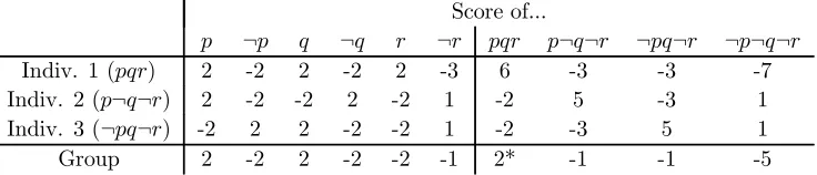
As an example, consider our doctrinal paradox agenda X = {p, q, r}± with n = 3
individuals, and suppose the quota rule departs only slightly from propositionwise majority voting: all propositionst inX\{¬r}keep a majority threshold ofmt= 2, but¬rreceives
a unanimity threshold m¬r = 3. This quota rule manages to never generate logically
inconsistent collective judgment sets,15 but does so at the expense of allowing collective
incompleteness. Indeed, for our example profile, the quota rule returns the collective judgment setpq, which is silent on the choice betweenrnor¬r. As illustrated in Table 5, the scoring rule w.r.t. (11) restores collective rationality by leading to the premise-based
Score of...
p ¬p q ¬q r ¬r pqr p¬q¬r ¬pq¬r ¬p¬q¬r
Indiv. 1 (pqr) 2 -2 2 -2 2 -3 6 -3 -3 -7 Indiv. 2 (p¬q¬r) 2 -2 -2 2 -2 1 -2 5 -3 1 Indiv. 3 (¬pq¬r) -2 2 2 -2 -2 1 -2 -3 5 1
[image:16.595.114.482.313.392.2]Group 2 -2 2 -2 -2 -1 2* -1 -1 -5
Table 5: Scoring (11) for the doctrinal paradox agenda and profile
outcomepqr. To read the table, note that scoring (11) is given bys+(t) = 2ands−(t) =−2
for alltinX\{¬r},s+(¬r) = 1ands−(¬r) =−3.
How does our scoring rule ‘repair’ those special quota rules which use a uniform thresh-old m≡mp(p∈X), such as majority rule?
Remark 3 For a uniform threshold m ≡mp, the scoring rule w.r.t. scoring (11) is the
Hamming rule, or equivalently, the simple scoring rule.
This remark follows from Proposition 1 and the fact that, for a uniform threshold
m≡mp, scoring (11) is equivalent to simple scoring by footnote 6.
Finally, I note that the scoring rules w.r.t. (11) is not the only scoring rule which can ‘repair’ the quota ruleF(mp)p∈X — though it might be the most plausible one, as long as we
do not wish to introduce additional parameters. If, however, we are prepared to introduce additional parameters, scoring (11) can be generalized: for each p ∈ X let αp > 0be a
coefficient measuring how important it is that the scoring rule is faithful to the quota rule’s collective judgment onp; and let scoring be defined by
sA(p) =
s+(p) =αp(n+ 1−mp) ifp∈A
s−(p) =−αpmp ifp∈A.
(12)
The earlier scoring (11) is obviously a special case in which all αp are 1. Proposition
5 still holds for this generalized kind of propositionwise scoring. The scoring rule will tend to match the quota rule on propositionspwith high importance coefficientαp, while
modifying (‘repairing’) the quota rule at propositionspwith lowαp.
3.7
Premise- and conclusion-based aggregation
I have just mentioned the possibility of a differential treatment of propositions when ‘re-pairing’ a quota rule. This possibility is particularly salient in the popular context of premise- or conclusion-based aggregation.16 One may indeed view the classical
premise-and conclusion-based rules as two (rival) ways of repairing the simplest of all quota rules — majority rule — by privileging certain propositions over others, namely premise propositions or conclusion propositions, respectively.
Let me put this precisely. Consider majority voting, i.e., the quota rule with a uniform majority threshold m ≡mp (the smallest integer above n/2). To restore collective
ratio-nality, we again endow each proposition p∈X with a ‘coefficient of importance’, but now let this coefficient be determined by whetherphas a ‘premise’ or ‘conclusion’ status. For-mally, suppose the agenda is partitioned into two negation-closed sets, the setPof ‘premise propositions’ and the set X\P of ‘conclusion propositions’. In the case of our doctrinal paradox agendaX={p, q, r}±, we haveP={p, q}±. Each premise propositionp∈P has
the importance coefficient αp ≡ αpremise, and each conclusion propositionp ∈ X\P has
the importance coefficient αp ≡αconclusion, for fixed parameters αpremise, αconclusion ≥ 0.
In this scenario, the scoring (12) becomes equivalent (by footnote 6) to the scoring given by
sA(p) =
αpremise for accepted premise propositionsp∈A∩P
αconclusion for accepted conclusion propositionsp∈A\P
0 for rejected propositionsp∈A.
(13)
By calibrating the two importance coefficients, we can influence the relative weights of premises and conclusions. If we givefar moreimportance to premise propositions (αpremise≫
αcoclusion) or to conclusion propositions (αcoclusion≫αpremise), the scoring rule reduces to
the premise- or conclusion-based rule, respectively. To substantiate this claim, one needs to define both rules. For simplicity, I restrict attention to our doctrinal paradox agenda
X ={p, q, r}± withP ={p, q}± (though more generalX and P could be considered17).
In this case, assuming for simplicity that the group size nis odd,
• thepremise-based rule is the aggregation rule which for each profile in Dn delivers
the (unique) judgment set in D containing each premise proposition accepted by a majority;
• theconclusion-based rule is the aggregation rule which for each profile inDndelivers
the judgment set (or sets) inDcontaining the conclusion proposition accepted by a majority.18
These two rules have the following characterizations as scoring rules:
1 6See for instance List (2004), Dietrich and Mongin (2010) and Nehring and Puppe (2010b).
1 7Our analysis generalizes easily to anyXandP such that (i) the premise propositions inPare logically
independent, and (ii) complete judgments across the premise propositions in P uniquely determine the judgments on the conclusion propositions inX\P.
Remark 4 For our doctrinal paradox agendaX={p, q, r}± with set of premise proposi-tions P={p, q}±, and for an odd group size, the scoring rule w.r.t. scoring (13) is
• the premise-based rule if and only if αpremise>(n−2)αconclusion, • the conclusion-based rule if and only ifαconclusion> αpremise= 0.
This result lets premise- and conclusion-based aggregation appear in a rather ex-treme light: each rule is based on somewhat unequal importance coefficients αpremise and
αconclusion, deeming one type of proposition to be overwhelmingly more important than
the other. It might therefore be interesting to consider more equilibrated values of the importance coefficients, so as to achieve a compromise between democracy at the premise level and democracy at the conclusion level.
4
Set scoring rules: assigning scores to entire judgment
sets
An interesting generalization of scoring rules is obtained by assigning scores directly to entire judgment sets rather than single propositions. Aset scoring function— or simplyset scoring — is a functionσwhich to every pair of rational judgment setsC andA assigns a real numberσA(C), thescore ofCgivenA, which measures how wellCperforms (‘scores’)
from the perspective of holding the judgment setA. Formally,σ:D × D →R. The most elementary example, to be callednaive set scoring, is given by
σA(C) = 1 ifC=A
0 ifC=A. (14)
Any set scoring σ gives rise to an aggregation rule Fσ, the set scoring rule (or
general-ized scoring rule) w.r.t. σ, which for each profile (A1, ..., An)∈ Dn selects the collective
judgment set(s) C inDhaving maximal sum-total score across individuals:
Fσ(A1, ..., An) = argmaxC∈D
i∈N
σAi(C).
An aggregation rule is a set scoring rule simpliciter if it is the set scoring rule w.r.t. to some set scoringσ. Set scoring rules generalize ordinary scoring rules, since to any ordinary scoringscorresponds a set scoringσ, given by
σA(C)≡ p∈C
sA(p),
and the ordinary scoring rule w.r.t. scoincides with the set scoring rule w.r.t. σ.
4.1
Naive set scoring and plurality voting
Plurality rule is the aggregation ruleF which for every profile (A1, ..., An)∈ Dn declares
the most often submitted judgment set(s) as the collective judgment set(s):
F(A1, ..., An) = most frequently submitted judgment set(s)
This rule is of course normatively questionable;19 but it deserves our attention, if only
because of its simplicity and the recognized importance of plurality voting in social choice theory more broadly. Plurality rule can be construed as a set scoring rule:
Remark 5 The naive set scoring rule is plurality rule.
4.2
Distance-based set scoring
Set scoring rules generalize distance-based aggregation. Given an arbitrary distance func-tion d over D (not necessarily the Hamming-distance), all that is needed is to consider what I call distance-based set scoring, defined by
σA(C) =−d(C, A). (15)
So, C scores high if it is close to the judgment set held, A. This renders sum-score-maximization equivalent to sum-distance-minimization:
Remark 6 For every given distance function overD, the distance-based set scoring rule is the distance-based rule.
So, all distance-based rules can be modelled as set scoring rules (but not vice versa20).
As an example, consider the so-called discrete distance,21 defined by
d(A, B) = 0 ifA=B
1 ifA=B.
Here, distance-based set scoring (15) is equivalent to naive set scoring (14), since the two differ only by a constant (of one). So, joining Remarks 5 and 6, we may view plurality rule either as the naive set scoring rule or as the discrete-distance-based rule.
4.3
Approximating the ‘average voter’
Given an ordinary scoring s, we have so far aimed for collective judgments with high total score. But this is not the only plausible aim or approach. We now turn to an altogether different approach. Rather than using s to assign scores only from each individual’s per-spective, we now care about how propositions score under the collective judgment set. Instead of wanting the collective judgments to get highest total score from individuals, we now want them to resemble an ‘average individual’s judgments’ in the sense that the collective judgments should lead (approximately) to the same scores of propositions as the individual judgments do on average. In short, any propositionp’s collective score should be (approximately) p’s average individual score. This approach has its own, rather different intuitive appeal. But is it really totally different? As will turn out, aggregation rules which
1 9It ignores the internal structure of judgment sets, hence ‘throws away’ much information. 2 0In trying to re-model an arbitrary set scoring ruleF
σ as a distance-based rule, one might be tempted
to define the ‘distance’ betweenAandBasdσ(A, B) :=σA(A)−σA(B). Ifdσturns out to define a proper
distance function (see fn. 7), then we obtain a distance-based ruleFdσ, which coincides with the set scoring
ruleFσ. But for many plausible set scoringsσ,dσhas little in common with a distance function, violating
up to all three axioms, notably symmetry and the triangle inequality.
2 1This metric derives its name from the fact that it induces the discrete topology on whatever set it is
follow this approach — I call them ‘average-score rules’ as opposed to ‘scoring rules’ — can be viewed as a particular kind of set scoring rules. This result is in fact a special case of a powerful precursor result by Zwicker (2008), as Marcus Pivato kindly pointed out to me.22
Given an ordinary scorings, we can represent judgment sets inDas vectors inRX, by identifying each judgment setAinDwith itsscore vector, i.e., the vector inRX whosepth
component is the score of p,sA(p).23 The score vector corresponding toA∈ Dis denoted
As≡(s
A(p))p∈X ∈RX. Having represented judgment sets as vectors of numbers, we can
apply standard algebraic and geometric operations, such as adding judgment sets, taking their average, or measuring their distance — where, of course, sums or averages of (score vectors of) judgment sets in D may be ‘infeasible’, i.e., not correspond to any judgment set inD.
Theaverage-score rule w.r.t. scorings is defined as the aggregation ruleF which for every profile (A1, ..., An) ∈ Dn chooses the collective judgment set(s) whose score vector
comes closest to the group’s average score vector 1
n i∈NAsi in the sense of Euclidean
distance inRX:
F(A1, ..., An) = j.s. closest to the average individual j.s. in score vector terms
= argminC∈D Cs−n1 i∈N
Asi .
Viewed geometrically as an operation in RX, the collective score vector is the orthogonal projection of the average score vector 1
n iAsi on the set Ds ≡ {As : A ∈ D} ⊆RX of
feasible score vectors.24
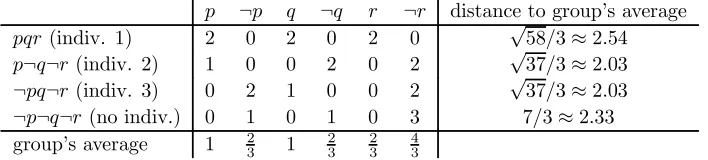
[image:20.595.117.481.291.338.2]As an illustration, consider once again reversal scoring for our doctrinal paradox agenda. Table 6 reports the score vector of each judgment set (including the one not submitted by
p ¬p q ¬q r ¬r distance to group’s average
pqr(indiv. 1) 2 0 2 0 2 0 √58/3≈2.54
p¬q¬r(indiv. 2) 1 0 0 2 0 2 √37/3≈2.03
¬pq¬r(indiv. 3) 0 2 1 0 0 2 √37/3≈2.03
¬p¬q¬r(no indiv.) 0 1 0 1 0 3 7/3≈2.33
group’s average 1 2
3 1 23 23 43
Table 6: The average-score rule (w.r.t. reversal scoring) for the doctrinal paradox agenda and profile
any individual), and its distance to the group’s average score vector. By minimizing this distance, the rule delivers a tie between the two conclusion-based outcomes p¬q¬r and
¬pq¬r. The premise-based outcomepqrlooks worse than ever: it is even farther from the average than the never-submitted outcome¬p¬q¬r.
Now that we have two rival ways of aggregating based on a scoring s — namely, the scoring rule and the average-score rule — the question is whether any connection can be
2 2Average-score rules are special cases of Zwicker’s ‘mean proximity rules’ in his abstract, more
gen-eral aggregation framework. Zwicker’s Theorem 4.2.1 (more precisely, its proof) reveals that any ‘mean proximity rule’ can be given a representation which essentially corresponds to our representation of an average-score rule in Proposition 6.
2 3This identification is one-to-one as long as the scoring has the (very plausible) property thats
A(p)>
sA(¬p)wheneverp∈A.
2 4Formally,F(A
1, ..., An)s= PROJDs(1
n iAsi), where the orthogonal projection ofx∈R
XonY ⊆RX
[image:20.595.121.475.420.500.2]established. The average-score rule can be construed as aset scoring rule, namely in virtue of the set scoring given by
σA(C) =− Cs−As 2. (16)
Here,Cis taken to score high if it is close toAin terms of thesquared Euclidean distance of score vectors.
Proposition 6 For any scoring s, the average-score rule w.r.t. s is the set scoring rule w.r.t. set scoring (16).
As an application, lets be simple scoring (1). Here, the set scoring (16) is expressible as an increasing affine transformation of the set scoring corresponding to simple scoring, i.e., of the set scoring σ′ given by25
σ′A(C) =
p∈C
sA(p) =|C∩A|.
So, the set scoring rule Fσ coincides with the simple scoring ruleFs, and hence with the
Hamming rule FdH a m by Proposition 1. Thus, as a corollary of Propositions 1 and 6, the
Hamming rule can be characterized not just as a scoring rule but also as an average-score rule, both times using the same scoring:
Corollary 2 The Hamming rule is the scoring rule and the average-score rule, both times w.r.t. simple scoring.
4.4
Probability-based set scoring
I close the analysis by taking a brief (skippable) excursion into an important, but differ-ent approach to judgmdiffer-ent aggregation: the epistemic or truth-tracking approach. In this approach, each propositionp∈X is taken to have an objective, but unknown truth value (‘true’ or ‘false’), and the goal of aggregation is to track the truth, i.e., to generate true collective judgments.26 The truth-tracking perspective has a long history elsewhere in
so-cial choice theory (e.g., Condorcet 1785, Grofman et al. 1983, Austen-Smith and Banks 1996, Dietrich 2006b, Pivato 2011a); but within judgment aggregation theory specifically, rather little work has been done on the epistemic side (e.g., Bovens and Rabinowicz 2006b, List 2005, Bozbay et al. 2011).
The epistemic approach warrants the use of particular set scoring rules. To show this, I import standard statistical estimation techniques (such as maximum-likelihood estimation), following the path taken by other authors in the context of preference aggregation (e.g., Young 1995) and other aggregation problems (e.g., Dietrich 2006b, Pivato 2011a). My goal is to give no more than a brief introduction to what could be done. The results given below are essentially variants of existing results; see in particular Pivato (2011a).27
2 5Sinceσ
A(C) =− |C△A|
2
=− |C△A|=−2|C\A|=−2 (|C| − |C∩A|) =− |X|+ 2|C∩A|. 2 6The epistemic perspective is usually contrasted with theproceduralperspective, which takes the goal of aggregation to be to generate collective judgments which reflect the individuals’ judgments in a procedurally fair way. To illustrate the contrast between the two perspectives, suppose that all individuals hold the same judgment set A. Then Ais clearly the right collective judgment set from the perspective of procedural fairness. But from an epistemic perspective, all depends on whether people’s unanimous endorsement of Ais sufficient evidence forAbeing true.
For each combination(A1, ..., An, T)∈ Dn×Dofn+1judgment sets, letPr(A1, ..., An, T)
>0measure the probability that people submit the profile(A1, ..., An)and the set of true
propositions is T, where of course (A1,...,An,T)∈Dn×DPr(A1, ..., An, T) = 1. From this
joint probability function we can, as usual, derive various marginal and conditional prob-abilities, such as the probability that the truth isT ∈ D,Pr(T) = (A1,...,A
n)∈DnPr(A1, ...,
An, T), the probability that the profile is(A1, ..., An),Pr(A1, ..., An) = T∈DPr(A1, ..., An,
T), the conditional probabilityPr(T|A1, ..., An) = Pr(A
1,...,An,T)
Pr(A1,...,An) (called theposterior
prob-ability ofT given the ‘data’A1, ..., An), and the conditional probabilityPr(A1, ..., An|T) = Pr(A1,...,An,T)
Pr(T) (called thelikelihood of the ‘data’A1, ..., An givenT).
Themaximum-likelihood ruleis the aggregation ruleF:Dn⇒Dwhich for each profile
(A1, ..., An) ∈ Dn defines the collective judgments such that their truth would make the
observed profile (‘data’) maximally likely:
F(A1, ..., An) = argmaxT∈DPr(A1, ..., An|T).
The maximum-posterior rule is the aggregation rule F : Dn ⇒D which for each profile
(A1, ..., An)∈ Dn defines the collective judgments such that they have maximal posterior
probability of truth conditional on the observed profile (‘data’):
F(A1, ..., An) = argmaxT∈DPr(T|A1, ..., An).
Both of these rules correspond to well-established statistical estimation procedures. Let us now make two standard, but restrictive assumptions on probabilities. We assume that voters are ‘independent’ and ‘equally competent’ (in analogy to the assumptions of Condorcet’s classical jury theorem28). Formally, for everyT ∈ D,
(IND) the individual judgment sets are independent conditional onT being the true judg-ment set, i.e., Pr(A1, ..., An|T) = Pr(A1|T)· · ·Pr(An|T) for all A1, ..., An ∈ D (‘
in-dependence’)
(COM) for each A ∈ D, each individual has the same probability, denoted Pr(A|T), of submitting the judgment setAconditional onT being the true judgment set (‘equal competence’).
Condition (COM) in particular implies that individuals have the same (conditional) probability of holding the true judgment set; but nothing is assumed about the size of this probability of ‘getting it right’. The just-defined aggregation rules turn out to be set scoring rules in virtue of defining the score of T ∈ DgivenA∈ Dby, respectively,
σA(T) = log Pr(A|T) (17)
σA(T) = log Pr(A|T) +
1
nlog Pr(T). (18)
Proposition 7 If voters are independent (IND) and equally competent (COM), then
• the maximum-likelihood rule is the set scoring rule w.r.t. set scoring (17),
• the maximum-posterior rule is the set scoring w.r.t. set scoring (18).
2 8The classical Condorcet jury theorem is essentially concerned with a simple judgment aggregation
5
Concluding remarks
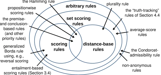
I hope to have convinced the reader that scoring rules, and more generally set scoring rules, form interesting positive solutions to the judgment aggregation problem. They for instance allow us to generalize Borda aggregation to judgment aggregation (the simplest method being to use reversal scoring). Figure 1 summarizes where we stand by depicting different classes of rules (scoring rules, set scoring rules, and distance-based rules) and positioning several concrete rules (such as Hamming rule). While the positions of most
arbitrary rules
distance-base rules scoring
rules
set scoring rules
the Condorcet-admissibility rule the “truth-tracking” rules of Section 4.4 the Hamming rule
generalized Borda rule using, e.g., reversal scoring
non-anonymous rules plurality rule propositionwise
scoring rules
entailment-based scoring rules (Section 3.4)
average-score rules the
premise-and conclusion-based rules
[image:23.595.129.469.201.361.2](and other priority rules)
Figure 1: A map of judgment aggregation possibilities
rules in Figure 1 have been established above or follow easily, a few positions are of the order of conjectures. This is so for the placement of our Borda generalizationoutside the class of distance-based rules.29
Though several old and new aggregation rules are scoring rules (or at least set scoring rules), there are important counterexamples. One counterexample is the mentioned rule introduced by Nehring et al. (2011) (the so-called Condorcet-admissibility rule, which generates rational judgment set(s) that ‘approximate’ the majority judgment set). Other counterexamples are non-anonymous rules (such as rules prioritizing experts), and rules that return boundedly rational collective judgments (such as rules returning incomplete but still consistent and deductively closed judgments). The last two kinds of counterexamples suggest two generalizations of the notion of a scoring rule. Firstly, scoring might be allowed to depend on the individual; this leads to ‘non-anonymous scoring rules’. Secondly, the search for a collective judgment set with maximal total score might be done within a larger set than the setDof fully rational judgment sets (such as the set of consistent but possibly incomplete judgment sets); this leads to ‘boundedly rational scoring rules’. The same generalizations could of course be made for set scoring rules. Much work is ahead of us.
2 9For technical correctness, I also note two details about how to read Figure 1. First, for trivial agendas,
such as a single-issue agenda X = {p,¬p}, several rules of course become equivalent, and distinctions drawn in Figure 1 disappear. More precisely, by positioning a rule outside a class of rules (e.g., by positioning plurality rule outside the class of scoring rules), I am of course not implying that for all