Risk Parity Portfolios with Risk Factors
Roncalli, Thierry and Weisang, Guillaume
Evry University, Clark University
15 September 2012
Online at
https://mpra.ub.uni-muenchen.de/44017/
Thierry Roncalli
Research & Development
Lyxor Asset Management
thierry.roncalli@lyxor.com
Guillaume Weisang
Graduate School of Management
Clark University, Worcester, MA
gweisang@clarku.edu
This version: September 2012
(Work in Progress)
Abstract
Portfolio construction and risk budgeting are the focus of many studies by aca-demics and practitioners. In particular, diversification has spawn much interest and has been defined very differently. In this paper, we analyze a method to achieve port-folio diversification based on the decomposition of the portport-folio’s risk into risk factor contributions. First, we expose the relationship between risk factor and asset contri-butions. Secondly, we formulate the diversification problem in terms of risk factors as an optimization program. Finally, we illustrate our methodology with some real life examples and backtests, which are: budgeting the risk of Fama-French equity factors, maximizing the diversification of an hedge fund portfolio and building a strategic asset allocation based on economic factors.
Keywords: risk parity, risk budgeting, factor model, ERC portfolio, diversification, con-centration, Fama-French model, hedge fund allocation, strategic asset allocation.
JEL classification: G11, C58, C60.
1
Introduction
While Markowitz’s insights on diversification live on, practical limitations to direct imple-mentations of his original approach have recently lead to the rise of heuristic approaches. Approaches such as weighted, minimum variance, most diversified portfolio, equally-weighted risk contributions, risk budgeting or diversified risk parity strategies have be-come attractive to academic and practitioners alike (see e.g. Meucci, 2007; Choueifaty and Coignard, 2008; Meucci, 2009; Maillardet al., 2010; Bruder and Roncalli, 2012; Lohre et al., 2012) for they provide elegant and systematic methodologies to tackle the construction of diversified portfolios.
While explicitly pursuing diversification, portfolios constructed with the methodologies cited above may well lead to solutions with unfortunately hidden risk concentration. Meucci (2009)’s work on diversification across principal component factors provided a clue to re-solving this unfortunate problem by focusing on underlying risk factors. In this paper, we build on this idea and combine it with the risk-budgeting approach of Bruder and Roncalli
(2012) to develop a risk-budgeting methodology focused on risk factors. When used with the objective of maximizing risk diversification, our approach is tantamount to diversifying across the ‘true’ sources of risk and often leads to a solution with equally-weighted risk factor contributions. Hence, we dubbed it the ‘risk factor parity’ approach.
This methodology is however more versatile. In this paper, we make explicit the relations between any risk factor and asset contributions to portfolio risk. And, in particular, we show that the equally-weighted risk factor contributions approach is equivalent to a risk-budgeting solution on the assets of the portfolio with a specific risk budgets profile. We also examine different optimization programs to obtain the desired outcome.
The plan of this paper is thus as follows. Section 2 provides a couple of motivating ex-amples. In Section 3, we derive the relations between asset and risk factors contributions to overall risk, and provide some illustrations. In Section 4, we consider two types of portfolio construction methodologies, first by matching risk contributions and second by minimizing a concentration index. Finally, Section 5 provides three applications of our portfolio con-struction methodologies: one in the context of risk budgeting on equity risk factors, a second on portfolios of hedge funds, and finally an application to strategic allocation.
2
Motivations
2.1
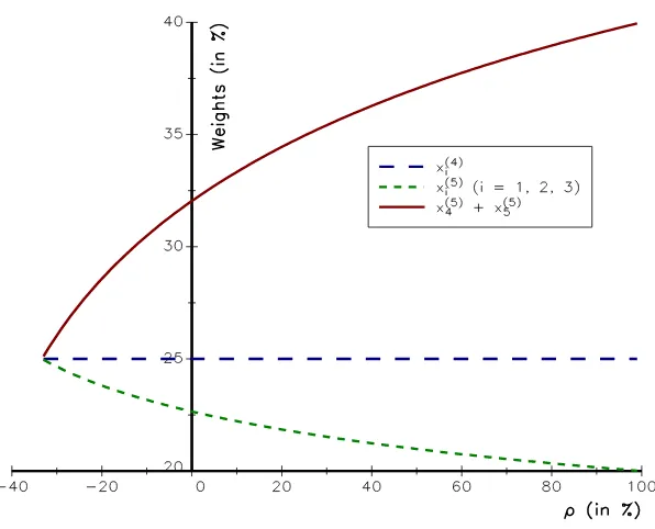
On the importance of the asset universe
Let’s consider a universe of4assets with equal volatilities and a uniform correlationρ. In this case, the equally-weighted risk contribution (ERC) portfoliox(4)corresponds to the equally-weighted portfolio. Let’s add to this universe a fifth asset with equal volatility. We assume that this asset is perfectly correlated with the fourth asset. In that case, the composition of the ERC portfoliox(5) depends on the value of the correlation coefficientρ. For example, if the cross-correlationρbetween the first four assets is zero, the ERC portfolio’s composition is given by x(5)i = 22.65% for the three first assets, while x
(5)
i = 16.02% for the two last
assets.
Such a solution could be confusing to a professional since in reality there are only four and not five assets in our universe1. A financial professional would expect the sum of the
exposures to the fourth and fifth assets to equal the exposure to each of the first three assets, i.ex(5)4 +x
(5)
4 = 25%. And, the weights of the assets four and five are therefore equal to the weight of the fourth asset in the 4-assets universe divided by 2 –x(5)5 =x
(5) 4 =x
(4) 4 /2 =
12.5%. However, this solution is reached only when the correlation coefficient ρ is at its lowest value2 as shown in Figure 1.
This example shows that the asset universe is an important factor when considering risk parity portfolios. Of course, this is a toy example, but similar issues arise in practice. Let’s consider multi-asset classes universes. If the universe includes5 equity indices and5 bond indices, then the ERC portfolio will be well balanced between equity and bond in terms of risk. Conversely, if the universe includes 7 equity indices and 3 bond indices, the equity risk of the ERC portfolio represents then 70% of the portfolio’s total risk, a solution very unbalanced between equity and bond risks.
1
The fourth and fifth assets are in fact the same since ρ4,5 = 1. This problem is also known as the
duplication invariance problem (Choueifatyet al., 2011).
2
2.2
Which risk would you like to diversify?
We consider a set ofmprimary assets (A′ 1, . . . ,A
′
m)with a covariance matrixΩ. We now definensynthetic assets(A1, . . . ,An)which are composed of the primary assets. We denote
W = (wi,j)the weight matrix such that wi,j is the weight of the primary asset A
′
j in the
synthetic asset Ai. Indeed, the synthetic assets could be interpreted as portfolios of the
primary assets. For example,A′
j may represent a stock whereas Ai may be an index. By
construction, we have∑n
i=1wi,j = 1. It comes that the covariance matrix of the synthetic
assetsΣis equal toWΩW⊤ .
We now consider a portfoliox= (x1, . . . , xn)defined with respect to the synthetic assets.
The volatility of this portfolio is thenσ(x) =√x⊤Σx. We deduce that the risk contribution of the synthetic assetiis:
RC(Ai) =xi (Σx)i
√
x⊤Σx
We could also defined the portfolio with respect to the primary assets. In this case, the composition isy = (y1, . . . , ym) where yj =∑
n
i=1xiwi,j. In a matrix form, we have y =
W⊤
x. In a similar way, we may compute the risk contribution of the primary assetsj:
RC(
A′
j
)
=yj (Ωy)j
√
y⊤Ωy
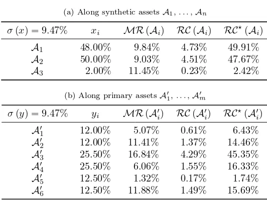
[image:4.612.150.448.130.371.2]We consider three equally-weighted synthetic assets with:
W =
1/4 1/4 1/4 1/4
1/4 1/4 1/4 1/4 1/2 1/2
First, let’s consider portfolio#1with synthetic assets’ weights of36%,38%and26% respec-tively. The risk contributions of these positions to the volatility of portfolio#1is provided in Table 1a. Notice that this portfolio is very close to the ERC portfolio. It is well-balanced in terms of risk with respect to the synthetic assets. However, if we analyze this portfolio in terms of primary assets (cf. Table 1b), about 80% of the risk of the portfolio is then concentrated on the third and fourth primary assets. We have here a paradoxical situation. Depending on the analysis, this portfolio is either well diversified or is a risk concentrated portfolio. Let’s now consider portfolio#2 with synthetic weights48%, 50% and2%. The risk contributions for this portfolio are provided in Table 2. In this case, the portfolio is not very well balanced in terms of risk, because the two first assets represent more than97%
of the risk of the portfolio, whereas the risk contribution of the third asset is less than3%
(cf. Table 2a). This portfolio is thus far from the ERC portfolio. However, an analysis in terms of the primary assets, shows that this portfolio is less concentrated than the previous one (cf. Table 2b). The average risk contribution is 16.67%. Notice that primary assets which have a risk contribution above (resp. below) this level in the first portfolio have a risk contribution that decreases (resp. increases) in the second portfolio. In Figure 2, we have reported the Lorenz curve of the risk contributions of these two portfolios with respect to the primary and synthetic assets. We verify that the second portfolio is less concentrated in terms of primary risk.
Table 1: Risk decomposition of portfolio #1
(a) Along synthetic assetsA1, . . . ,An
σ(x) = 10.19% xi MR(Ai) RC(Ai) RC⋆(Ai)
A1 36.00% 9.44% 3.40% 33.33%
A2 38.00% 8.90% 3.38% 33.17%
A3 26.00% 13.13% 3.41% 33.50%
(b) Along primary assetsA′
1, . . . ,A′m
σ(y) = 10.19% yi MR(A
′
i) RC(A
′
i) RC ⋆
(A′
i)
A′
1 9.00% 3.53% 0.32% 3.12%
A′
2 9.00% 7.95% 0.72% 7.02%
A′
3 31.50% 19.31% 6.08% 59.69%
A′
4 31.50% 6.95% 2.19% 21.49%
A′
5 9.50% 0.93% 0.09% 0.87%
A′
6 9.50% 8.39% 0.80% 7.82%
Table 2: Decomposition of portfolio #2
(a) Along synthetic assetsA1, . . . ,An
σ(x) = 9.47% xi MR(Ai) RC(Ai) RC⋆(Ai)
A1 48.00% 9.84% 4.73% 49.91%
A2 50.00% 9.03% 4.51% 47.67%
A3 2.00% 11.45% 0.23% 2.42%
(b) Along primary assetsA′
1, . . . ,A′m
σ(y) = 9.47% yi MR(A′i) RC(A
′
i) RC ⋆(
A′
i)
A′
1 12.00% 5.07% 0.61% 6.43%
A′
2 12.00% 11.41% 1.37% 14.46%
A′
3 25.50% 16.84% 4.29% 45.35%
A′
4 25.50% 6.06% 1.55% 16.33%
A′
5 12.50% 1.32% 0.17% 1.74%
A′
6 12.50% 11.88% 1.49% 15.69%
[image:6.612.133.463.456.699.2]Remark 1. This second example is also related to the first example3. In the first example,
the right way to diversity is not to use the ERC portfolio, but different risk budgets b = (25%,25%,25%,12.5%,12.5%). In this case, we verify that we obtain the desired solution. The central question is then how to define properly these risk budgets.
3
Computing the risk decomposition with risk factors
3.1
The linear factor model
We consider a set of n assets {A1, . . . ,An} and a set of m risk factors {F1, . . . ,Fm}.
We denote by Rt the (n×1) vector of asset returns at time step t and Σ its associated
covariance matrix; and Ft the (m×1) vector of factor returns at t and Ω its associated
covariance matrix. We assume the following linear factor model:
Rt=AFt+εt (1)
with Ft and εt two uncorrelated random vectors. εt is an i.i.d. (n×1) centered random
vector of varianceD. Ais the(n×m)‘loadings’ matrix. Using (1), it is easy to deduce the following second-order relationship:
Σ =AΩA⊤
+D
At the portfolio level, we denote the portfolio’s asset exposures by the (n×1)vectorx and the portfolio’s risk factors exposures by the(m×1)vectory. These vectors are related through the P&L functionΠtof the portfolio at timet:
Πt=x⊤
Rt=x
⊤
AFt+x
⊤
εt=y
⊤
Ft+ηt
with4 y =A⊤
xand ηt =x⊤εt. Let’s note B =A⊤ and B+ the Moore-Penrose inverse of
B. We have therefore
x=B+y+e
wheree= (In−B+B)xis a (n×1)vector in the kernel ofB.
3.2
Defining the marginal risk contribution of factors
Let’s consider a convex risk measure R. We have R(x) = R(y, e). We notice that the idiosyncratic variableethat represents the specific risks of each asset position in the portfolio is a function of the portfolio compositionx. Thus, the marginal risk contributiondR(x)/dxi
of theithasset exposure is given as a function of the marginal risk contributiond
R(y, e)/dy of the factor exposures and the marginal risk contribution of the specific or idiosyncratic risk of assetidR(y, e)/deby5:
∂R(x)
∂ xi =
(
∂R(y, e)
∂ y B
)
i +
(
∂R(y, e)
∂ e
(
In−B+B
) )
i
3
In the first example, the problem comes from the fact that we have 5 assets, but only 4 factors.
4
By definition, we havecov (Ft, ηt) =0.
5
We have:
dR(x) dx =
∂R(y, e)
∂ y
dy
dx+
∂R(y, e)
∂ e
de
This decomposition is not very convenient however since it decomposes the(n×1)vectorx into a(m×1)vectory and a(n×1)error vectore. Another route is to write the following decomposition (Meucci, 2007):
x=(
B+ B˜+ ) (
y
˜
y
)
= ¯B⊤y¯ (2)
whereB˜+ is anyn×(n−m)matrix that spans the left nullspace ofB+. In this case, we could state the following theorem:
Theorem 1. The marginal risk contribution of assets are related to the marginal risk con-tribution of factors in the following way:
∂R(x)
∂ x =
∂R(x)
∂ y B+
∂R(x)
∂y˜ B˜
We deduce that the marginal risk contribution of thejth factor exposure is given by:
∂R(x)
∂ yj =
(
A+∂R(x)
∂ x⊤
)
j
For the additional factors, we have:
∂R(x)
∂y˜j =
(
˜
B∂R(x) ∂ x⊤
)
j
Proof. See Appendix A.2 page 29.
3.3
Euler decomposition of the risk measure
It is easy to verify that for any convex risk measure that verifies the Euler decomposition
R = ∂xR(x)·x = ∑in=1xi·∂xiR(x), the Euler decomposition is verified in the new coordinate system(y,y˜):
R(x) =∂R(x)
∂ y y+
∂R(x)
∂y˜ y˜
Let’s note RC(Fj) = yj ·∂yjR(x) the risk contribution of the factor j with respect to the riskR. Using Theorem 1, we find that the sum of the risk contributions of the factor exposures is simply expressed as:
m
∑
j=1
RC(Fj) =y
⊤∂R(x)
∂ y⊤ =x ⊤
(AA+)∂R(x)
∂ x⊤ (3)
whereAA+ = (B+B)⊤
is the orthogonal projector onto the range of B =A⊤
. We notice then that we do not retrieve all the risk measure if we only consider the risk contributions
of the factors: m
∑
j=1
RC(Fj)≤ R(x)
The difference is due to the additional factors:
R(x)− m
∑
j=1
RC(Fj) = n−m
∑
j=1
RC(F˜j
)
= x⊤( ˜B⊤B˜)∂R(x)
∂ x⊤
= x⊤
(In−AA+)
∂R(x)
If we consider the volatility of the portfolio, we obtain this result:
Theorem 2. When the risk measureR(x)is the volatility of the portfolioσ(x) =√x⊤
Σx, the risk contribution of thejth factor is:
RC(Fj) =
(
A⊤
x)
j·(A
+Σx)
j
σ(x)
For the risk factorsF˜t, the results become:
RC(F˜j
) = ( ˜ Bx) j· ( ˜
BΣx)
j
σ(x)
Proof. See Appendix A.3 page 30.
Remark 2. Theorems 1 and 2 are valid if the number of assetsnis larger than the number of factorsm. In the case wheren≤m, we obtain the same results, but the additional factors
˜
Fj vanish.
Remark 3. Using the previous results, we could define the risk contribution of the asset i
with respect to the risk factors. We have:
RC(Ai) =∂R(x)
∂ y Bei
(
e⊤
i B
+y+e⊤
i B˜
+y˜)+∂R(x)
∂y˜ Be˜ i
(
e⊤
i B
+y+e⊤
i B˜
+y˜)
In the casey˜= 0, this formula reduces to:
RC(Ai) =
(
∂R(x)
∂ y B+
∂R(x)
∂y˜ B˜
)
EiB+y
where Ei is a null matrix of dimension (n×n) except for the entry (i, i) which takes the
value one.
3.4
Some illustrations
3.4.1 The casen≥m
Let us consider an example with4assets and3 factors. The loadings matrix is:
A=
0.9 0 0.5 1.1 0.5 0 1.2 0.3 0.2 0.8 0.1 0.7
The three factors are uncorrelated and their volatilities are equal to20%, 10% and 10%. We consider a diagonal matrixD with specific volatilities 10%, 15%, 10% and 15%. The corresponding correlation matrix of asset returns is (in %):
ρ=
100.0 69.0 100.0 79.5 76.4 100.0 66.2 57.2 66.3 100.0
but not in terms of factors’ risk contributions. Indeed, the first factor represents more than
[image:10.612.162.437.210.391.2]80%of the risk. In the next section, we present a method in order to obtain portfolios which are more balanced with respect to factors.
Table 3: Risk decomposition of the equally-weighted portfolio
(a) Along assetsA1, . . . ,An
σ(x) = 21.40% xi MR(Ai) RC(Ai) RC⋆(Ai)
A1 25.00% 18.81% 4.70% 21.97%
A2 25.00% 23.72% 5.93% 27.71%
A3 25.00% 24.24% 6.06% 28.32%
A4 25.00% 18.83% 4.71% 22.00%
(b) Along factorsF1, . . . ,FmandF˜1, . . . ,F˜n−m
σ(y) = 27.45% yi MR(Fi) RC(Fi) RC⋆(Fi)
F1 100.00% 17.22% 17.22% 80.49%
F2 22.50% 9.07% 2.04% 9.53%
F3 35.00% 6.06% 2.12% 9.91%
˜
F1 2.75% 0.52% 0.01% 0.07%
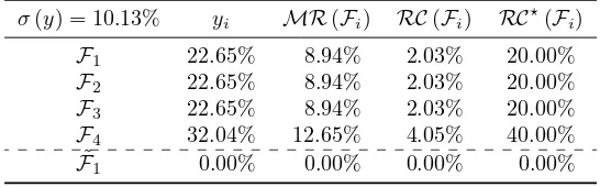
The casen≥mcorresponds also to our example in Section 2.1. We have4factors6with:
A=
[
I4 e⊤ 4
]
Ωis the covariance matrix of the first four assets while D is a matrix of zeros. If we use the framework developed in this section, we retrieve all the results. In particular, if we consider the ERC portfolio, we find that the three first factors have a contribution equal to20% whereas the fourth factor has a contribution of40%. In Table 4, we have reported the risk decomposition of the ERC portfolio with respect to the risk factors when the cross-correlation between the four first factors is equal to 0%. If we use another value for the correlation, results are different in terms of factor’ weights and risk contributions. But the relative risk contributionsRC⋆(
Fi)remain the same.
Table 4: Risk decomposition of the ERC portfolio with respect to risk factors
σ(y) = 10.13% yi MR(Fi) RC(Fi) RC⋆(Fi)
F1 22.65% 8.94% 2.03% 20.00%
F2 22.65% 8.94% 2.03% 20.00%
F3 22.65% 8.94% 2.03% 20.00%
F4 32.04% 12.65% 4.05% 40.00%
˜
F1 0.00% 0.00% 0.00% 0.00%
6
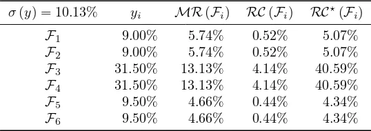
[image:10.612.162.435.613.698.2]3.4.2 The casen < m
This case corresponds to the example with primary and synthetic assets in Section 2.2. Indeed, the primary assets represent the risk factors. The loading matrix A is then equal to the weight matrixW, the covariance matrix of the factors is the covariance matrix of the primary assets whereas D is a matrix of zeros. In Table 5, we have reported the risk decomposition of the portfolio #1. We notice that the weight of the factor Fj is equal
to the weight of the primary assetA′
j, but we don’t obtain the same risk decomposition:
RC(Fi) ̸= RC(A′
i). The main reason is that the risk decomposition is not unique when
m > n. We face then an identification problem, which is a well-known problem in statistics. If we analyze the loading matrixA, we conclude that there is in fact three factors, because the primary assetsA′
1 andA ′
2 (resp. A ′ 5andA
′
6) influence together only the first synthetic assetA′
1(resp. the second synthetic assetA ′
2). In a same way, we notice a perfect symmetry between the primary assetsA′
3and A ′
4. This is why we deduce that the risk contributions of the factors satisfies this following system of equations:
RC(A′
1) +RC(A ′
2) =RC(F1) +RC(F2)
RC(A′
3) +RC(A ′
4) =RC(F3) +RC(F4)
RC(A′
5) +RC(A ′
6) =RC(F5) +RC(F6)
[image:11.612.164.433.424.519.2]It explains that only combination of factors could be identified, and not the factors them-selves.
Table 5: Risk decomposition of the portfolio #1 with respect to risk factors
σ(y) = 10.13% yi MR(Fi) RC(Fi) RC⋆(Fi)
F1 9.00% 5.74% 0.52% 5.07%
F2 9.00% 5.74% 0.52% 5.07%
F3 31.50% 13.13% 4.14% 40.59%
F4 31.50% 13.13% 4.14% 40.59%
F5 9.50% 4.66% 0.44% 4.34%
F6 9.50% 4.66% 0.44% 4.34%
4
Portfolio construction with factor risk budgeting
In this section, we consider two types of portfolio construction. In the first one, the allocation problem consists in matching some risk budgets with respect to risk factors. We show that the solution may not exist. This is why we consider a second approach which minimizes the risk concentration between the factors.
4.1
Matching the risk budgets
We would like to build a risk budgeting portfolio such that the risk contributions match a set of given risk budgets{b1, . . . , bm}:
This general problem can be formulated as a quadratic problem in a fashion similar to Bruder and Roncalli (2012):
(y⋆,yˆ⋆) = arg min m
∑
j=1
(RC(Fj)−bjR(y,y˜))2 (5)
u.c.
{ 1⊤
B+y+1⊤˜
B+y˜= 1 0≼B+y+ ˜B+y˜≼1
where≼denotes element-wise inequalities. If there is a solution to the optimization problem (5) and if the objective function is equal to zero at the optimum, it implies that it is also the solution of the matching problem (4). This problem (5) is however difficult to solve analytically as it involves PDE as its first-order conditions7. The following paragraphs
examine a related set of problems in which cases one can find an equivalent optimization problem in a more convenient form.
4.1.1 Non-negative risk factor allocation constraint
Bruder and Roncalli (2012) show that a problem of the form:
x⋆ = arg min
R(x) (6)
u.c.
RC(Ai) =biR(x)
1⊤
x= 1
x≽0
can be solved by considering the alternative problem:
z⋆ = arg min
R(z) (7)
u.c.
{ ∑n
i=1bilnzi≥c
z≽0
There exists then auniqueunnormalized solutionz⋆ and posingx⋆=z⋆/(1⊤
z⋆)
provides the optimal portfolio’s asset exposures.
Similarly, using the decomposition of the portfolio asset exposures x into factor risk exposure y given by Equation (2), the optimization problem with risk factor budgeting constraints can be formulated as:
(y⋆,y˜⋆) = arg min
R(y,y˜) (8)
u.c.
{ ∑m
j=1bjlnyj≥c
y≽0
We notice however that this problem induces a positivity constraint8on the risk factory.
The separation principle Note thaty˜is related to the idiosyncratic (or specific) risk of the portfolio. Indeed, we have:
x⊤
εt=ηt=e
⊤
Rt= ˜y
⊤˜
Ft
7
Nevertheless, we could solve it numerically using the SQP algorithm.
8
Ifyj≤0, we could replace the factorFjby a new factorFj′=−Fjmeaning thaty′j≥0. This is why
Since we focus in this paper on portfolio building controlling for the risk budgets associated with the risk factors, we will consider for now that we have an unconstrained minimization problem on the variable y˜, and will focus instead on solving the constrained optimization problem ony. Furthermore, it is always possible to solve a problem of the form (8) in two steps as long as the constraints ony andy˜are separate. We obtain:
y⋆ = arg min ˜
R(y) (9)
u.c.
{ ∑m
j=1bjlnyj≥c
y≽0
whereR˜(y) = infy˜R(y,y˜). The solution will be of the form(y⋆, ϕ(y⋆))wherey˜⋆=ϕ(y⋆) is solution to the first step of the optimization problem. The optimal portfolio allocationx⋆
is then recovered simply as:
x⋆=B+y⋆+ ˜B+ϕ(y⋆)
By construction, we also have9:
∂R˜ ∂ y(y) =
∂R
∂ y (y, ϕ(y)) and
∂R
∂y˜ (y, ϕ(y)) = 0
Application to the volatility risk measure For instance, if we measure the risk using the P&L volatility R(y,y˜) = σ(y,y˜), the problem is now equivalent to a quadratic opti-mization problem with constraints onyonly. Let us denoteΩ¯ the covariance matrix between factors. We have:
¯
Ω = cov(Ft,F˜t
)
=
(B+)⊤ΣB+ (B+)⊤Σ ˜B+
(
˜
B+) ⊤
ΣB+ (B˜+) ⊤
Σ ˜B+
=
( Ω Γ⊤
Γ Ω˜
)
Hence, we solve the augmented quadratic problem:
min y⊤Ωy+ ˜y⊤Ω˜˜y+ 2˜y⊤Γ⊤y
u.c.
{ ∑m
j=1bjlnyj ≥c
y≽0
in two steps, by first minimizing with respect toy˜, and then with respect toy. The solution of the first step is given byy˜=ϕ(y) =−Ω˜−1
Γ⊤
y. The problem is thus reduced to:
min y⊤
Sy
u.c.
{ ∑m
j=1bjlnyj≥c
y≽0
withS= Ω−Γ ˜Ω−1
Γ⊤
the Schur complement ofΩ˜. Because we haveΓ⊤
= (B+)⊤Σ ˜B+, we deduce that the optimal portfolio asset allocation is thus given by:
x⋆ = B+y⋆+ ˜B+ϕ(y⋆) = (B+−B˜+Ω˜−1(
B+)⊤
Σ ˜B+)y⋆
9
The second equality results from the definition ofϕas an infimum. The key to the first equality is being able to apply the chain rule, i.e. ϕbeing regular enough to be differentiable. Ifϕis a strict minimum and ifRis differentiable, then an application of the implicit function theorem to∂y˜R(y,y˜) = 0shows thatϕis
Remark 4. So long as the factors Ft andF˜t are uncorrelated (Γ = 0), a solution of the
form (y⋆,0) exists. In this case, the optimization problem could also be solved separately
on each of the orthogonal spaces: colA, as a constrained problem iny of the form (7), and
kerA, as an unconstrained minimization problem. The (un-normalized) asset allocation is given byx⋆=B+y⋆.
4.1.2 Adding long-only constraints
Additionally, if we want to consider long-only allocationsx, we must also include the fol-lowing constraint:
x=B+y+ ˜B+y˜≽0
The corresponding optimization problem is modified as follows:
(y⋆,y˜⋆) = arg min
R(y,y˜) (10)
u.c.
∑m
j=1bjlnyj≥c
y≽0
B+y+ ˜B+y˜≽0
We can again apply the separation principle10as in Section 4.1.1 and obtain this formulation:
(y⋆,y˜⋆) = arg min ˜R(y) (11)
u.c.
∑m
j=1bjlnyj≥c
y≽0
B+y+ ˜B+ϕ(y)
≽0
which is a convex optimization problem with a unique solution (if it exists) if, and only if, ϕis convex. It is easy to see that this condition is verified if we chooseRto be the P&L volatility. It is also true ifRis additively separable betweeny andy˜, in which caseϕ(y)is constant. This later situation should normally arise for some classic risk measures11 if the
factorsFtandF˜tare uncorrelated12(which depends only on the choice ofB˜+).
Remark 5. The solution may not exist even ifϕis convex.
Remark 6. An analysis presented in Appendix A.4 in the case whereRis the P&L volatility shows that the solution to formulation (9) will be solution to (11) as long as there exists
λ= (λx, λy)≽0such that:
(
A+−(B˜+)
⊤
Σ ˜Ω−1(B˜+)⊤)λ
x+λy= 0
According to this analysis, this condition is likely to be verified for some non trivial λ ∈
Rn++m. In such case, there exists ζ >0such that 0≤minyj≤ζ.
10
In general, the separation principle cannot be applied in cases where the constraints on(y,y˜)are not separate. However, in this case, ifϕis a strict minimum ofR, which is the case for the P&L volatility, then the two problems (10) and (11) are equivalent. Indeed, ify⋆ is solution to (11), then(y⋆, ϕ(y⋆))is
obviously a feasible point for (10). Conversely, if(y⋆⋆,y˜⋆⋆)is solution to (10), thenRbeing convex, any
local optimum has to be a global optimum. Therefore, we must have:
˜
R(y⋆⋆) =R(y⋆⋆,y˜⋆⋆) =R(y⋆⋆, ϕ(y⋆⋆)).
And, sinceϕis a strict minimum,(y⋆⋆,y˜⋆⋆) = (y⋆⋆, ϕ(y⋆⋆))and thus,B+y⋆⋆+ ˜B+ϕ
(y⋆⋆)≽0.
11
It is for example the case of value-at-risk and expected shortfall considering elliptic distributions or kernel estimation.
12
4.1.3 An illustration
[image:15.612.162.437.237.410.2]We consider the example with4 assets and3factors presented in Section 3.4.1 page 8. We have seen that the equally-weighted portfolio concentrates the risk on the first factor. We would like to build a portfolio with more balanced risk across the factors. For instance, ifb= (49%,25%,25%), we obtain the results given in Table 6. We notice that the corresponding portfolio presents positive weights.
Table 6: Matching the risk budgets(49%,25%,25%)
(a) Optimal solution(y⋆,y˜⋆)
σ(y) = 21.27% yi MR(Fi) RC(Fi) RC⋆(Fi)
F1 93.38% 11.16% 10.42% 49.00%
F2 24.02% 22.14% 5.32% 25.00%
F3 39.67% 13.41% 5.32% 25.00%
˜
F1 16.39% 1.30% 0.21% 1.00%
(b) Corresponding portfoliox⋆
σ(x) = 21.27% xi MR(Ai) RC(Ai) RC⋆(Ai)
A1 15.08% 17.44% 2.63% 12.36%
A2 38.38% 23.94% 9.19% 43.18%
A3 0.89% 21.82% 0.20% 0.92%
A4 45.65% 20.29% 9.26% 43.54%
We suppose now thatb = (19%,40%,40%). Results are reported in Table 7. We then obtain a long/short portfolio with a short position in the first asset. In Table 8, we report the solution to the optimization problem (5) if we impose that the weights of the portfolio are positive. At the optimum, the objective function is not equal to zero, meaning that there is no solution to the matching problem (4).
Table 7: Matching the risk budgets(19%,40%,40%)
(a) Optimal solution(y⋆,y˜⋆)
σ(y) = 23.41% yi MR(Fi) RC(Fi) RC⋆(Fi)
F1 92.90% 4.79% 4.45% 19.00%
F2 28.55% 32.79% 9.36% 40.00%
F3 45.21% 20.71% 9.36% 40.00%
˜
F1 −23.57% −0.99% 0.23% 1.00%
(b) Corresponding portfoliox⋆
σ(x) = 23.41% xi MR(Ai) RC(Ai) RC⋆(Ai)
A1 −26.19% 14.13% −3.70% −15.81%
A2 32.69% 21.21% 6.94% 29.63%
A3 14.28% 20.41% 2.91% 12.45%
[image:15.612.160.440.535.704.2](a) Optimal solution(y⋆,y˜⋆)
σ(y) = 21.82% yi MR(Fi) RC(Fi) RC⋆(Fi)
F1 89.85% 6.89% 6.19% 28.37%
F2 23.13% 28.67% 6.63% 30.40%
F3 47.02% 19.12% 8.99% 41.20%
˜
F1 2.53% 0.26% 0.01% 0.03%
(b) Corresponding portfoliox⋆
σ(x) = 21.82% xi MR(Ai) RC(Ai) RC⋆(Ai)
A1 0.00% 15.90% 0.00% 0.00%
A2 32.83% 22.03% 7.23% 33.15%
A3 0.00% 20.51% 0.00% 0.00%
A4 67.17% 21.72% 14.59% 66.85%
Remark 7. The existence problem of long-only portfolios could be easily illustrated with a portfolio of bonds. It is commonly argued that the three factors of the yield curve are the general level of interest rates, the slope of the yield curve and its convexity. Building a bond portfolio, for instance, where the slope and convexity factors have the same magnitude than the level factor is not possible if we impose that the weights are positive. In the long-only case, risk contributions of the slope and convexity factors are then bounded. We do not face this problem if the long-only constraint vanishes.
4.2
Minimizing the risk concentration between the risk factors
In the previous section, we have shown that the solution to the matching problem (4) does not necessarily exist. Of course, we could always optimize the problem (5) and consider the optimal solution without verifying that the objective function is equal to zero. In this case, we obtain the portfolio for which the risk contributions are the closest to the risk budgets in the sense of theL2 absolute norm13. We consider now a related problem:
RC(Fj)≃ RC(Fk)
The idea is to find a portfolio which is well balanced in terms of risk contributions with respect to the common factors. A first idea is to set bj =bk and to use use the previous
framework. Another way is to minimize the concentration between the risk contributions
(RC(F1), . . . ,RC(Fm)).
4.2.1 Concentration indexes
Letp∈Rn
+ such that 1 ⊤
p= 1. pis then a probability distribution. A probability distri-butionp+ is perfectly concentrated if there exists one observationi
0 such thatp+i0 = 1 and
13
If we prefer to use aL2relative norm, we could replace the objective function as follows:
(y⋆,y˜⋆) = arg min y
m
∑
j=1
m
∑
k=1
(RC
(Fj)
bj
−RC(Fk)
bk
[image:16.612.161.438.123.306.2]p+i = 0ifi̸=i0. As the opposite, a probability distributionp− such that p −
i = 1/n for all
i= 1, . . . , nhas no concentration. A concentration index is a mapping functionC(p)such thatC(p)increases with concentration and verifiesC(p−
)≤ C(p)≤ C(p+). Eventually, this index could be normalized such thatC(p−
) = 0andC(p+) = 1.
In our context, the vectorprepresents the risk contributions of the portfolio. C(p)will then measure the risk concentration of the portfolio with respect to the risk factors. The most popular methods to measure the concentration are the Herfindahl index and the Gini index. Another interesting statistic is the Shannon entropy which measures diversity, that is opposite of the concentration. Their definition is given below.
The Herfindahl index The Herfindahl index associated topis defined as:
H(p) = n
∑
i=1
p2i
This index takes the value1for a probability distributionp+and1/nfor a distribution with uniform probabilities. To scale the statistics onto[0,1], we consider the normalized index
H⋆(p)defined as follows:
H⋆(p) =nH(p)−1
n−1
The Gini index The Gini index measures the distance between the Lorenz curve of p and the Lorenz curve ofp−
. Its analytical expression is:
G(p) =2
∑n
i=1ipi:n
n∑n
i=1pi:n −
n+ 1
n
with{p1:n, . . . , pn:n} the ordered statistics of {p1, . . . , pn}. We verify that G(p−) = 0 and
G(p+) = 1
−1/n.
The Shannon entropy It is defined as follows:
I(p) =−
n
∑
i=1
pilnpi
When the Shannon entropy is used to measure the diversity, we prefer to consider the statisticI⋆(p) = exp (
I(p)). We notice thatI⋆(p−
) =nandI⋆(p+) = 1.
Remark 8. The entropy measure I⋆ is sometimes interpreted as the degree of
diversifica-tion, because it represents the true number of bets of the portfolio (Meucci, 2009). Another equivalent measure is the inverse of the Herfindal index.
4.2.2 An illustration
We continue our example by minimizing the risk concentration between the three risk factors. Results are given in Table 9. We notice that this portfolio satisfiesH⋆= 0,
G= 0andI⋆= 3
(a) Optimal solution(y⋆,y˜⋆)
σ(y) = 21.88% yi MR(Fi) RC(Fi) RC⋆(Fi)
F1 91.97% 7.91% 7.28% 33.26%
F2 25.78% 28.23% 7.28% 33.26%
F3 42.22% 17.24% 7.28% 33.26%
˜
F1 6.74% 0.70% 0.05% 0.21%
(b) Corresponding portfoliox⋆
σ(x) = 21.88% xi MR(Ai) RC(Ai) RC⋆(Ai)
A1 0.30% 16.11% 0.05% 0.22%
A2 39.37% 23.13% 9.11% 41.63%
A3 0.31% 20.93% 0.07% 0.30%
[image:18.612.163.436.123.305.2]A4 60.01% 21.09% 12.66% 57.85%
Table 10: Optimal portfolios withxi ≥10%
Criterion H(x) G(x) I(x)
x1 10.00% 10.00% 10.00%
x2 22.08% 18.24% 24.91%
x3 10.00% 10.00% 10.00%
x4 57.92% 61.76% 55.09%
H⋆ 0.0436 0.0490 0.0453
G 0.1570 0.1476 0.1639
I⋆ 2.8636 2.8416 2.8643
4.3
Solving some invariance problems
In this paragraph, we show that optimized risk parity portfolios with risk factors solve two important invariance problems.
4.3.1 The duplication invariance property
Let us come back to the first problem that has motivated this research. Choueifatyet al. (2011) show that the ERC portfolio does not verify the duplication invariance property, meaning that the ERC portfolio changes if we duplicate one asset.
Let Σ(n) be the covariance matrix of the n assets. We consider the RB portfolio x(n) corresponding to the risk budgetsb(n). We suppose now that we duplicate the last asset. In this case, the covariance matrix of then+ 1assets is:
Σ(n+1)=
(
Σ(n) Σ(n)e
n
e⊤
nΣ(n) 1
[image:18.612.208.390.361.470.2]We associate the factor model withΩ = Σ(n),D=0and:
A=
[
In
e⊤n
]
We consider the portfoliox(n+1) such that the risk contribution of the factors match the risk budgetsb(n). It is then easy to show that the matching portfolio verifiesy⋆ =x(n) in terms of factor weights. We have thenx(in+1) =x
(n)
i ifi < n and x
(n+1)
n +x(nn+1+1) =x (n)
n .
This result shows that an ERC portfolio verifies the duplication invariance property if the risk budgets are expressed with respect to factors and not to assets.
4.3.2 The polico invariance property
Choueifatyet al. (2011) suggest that a diversified portfolio should verify another desirable property called the polico invariance property:
“The addition of a positive linear combination of assets already belonging to the universe should not impact the portfolio’s weights to the original assets, as they were already available in the original universe. We abbreviate ‘positive linear combination’ to read Polico.”
We use the previous framework and introduce an assetn+ 1which is a linear (normalized) combinationαof the firstnassets. In this case, the covariance matrix of then+ 1assets is:
Σ(n+1)=( Σ(n) Σ(n)α
α⊤
Σ(n) α⊤
Σ(n)α
)
We associate the factor model withΩ = Σ(n),D=0and:
A=
[
In
α⊤
]
We consider the portfoliox(n+1) such that the risk contribution of the factors match the risk budgetsb(n). It is then easy to show that the factor weights of the matching portfolio satisfy:
y⋆=
[
A+x(n)
0
]
We have then x(n+1) = Ay⋆, which implies that x(n)
i = x
(n+1)
i +αix
(n+1)
n+1 if i ≤ n. This result shows that a RB portfolio (and so an ERC portfolio) verifies the polico invariance property if the risk budgets are expressed with respect to factors and not to assets.
Remark 9. This result is related to our example with primary and synthetic assets.
5
Applications
5.1
Budgeting the Fama-French-Carhart factors
LetRibe the return of theithasset andRf be the risk-free rate. In the capital asset pricing
model (CAPM) of Sharpe (1964), we have:
E[Ri] =Rf+βi(E[RMKT]−Rf)
whereRMKT is the return of the market portfolio and βi is the measure of the systematic
risk defined by:
βi =
cov (Ri, RMKT)
var (RMKT)
This model is also called the one-factor pricing model, because the stock return is entirely explained by one common risk factor represented by the market. According to Fama and French (2004), this model is the centerpiece of MBA investment courses and is widely used in finance by practitioners despite a large body of evidence in the academic literature of the invalidation of this model:
“The attraction of the CAPM is that it offers powerful and intuitively pleasing predictions about how to measure risk and the relation between expected return and risk. Unfortunately, the empirical record of the model is poor – poor enough to invalidate the way it is used in applications.” (Fama and French, 2004, p. 25)
In 1992, Fama and French studied several factors to explain average returns (size, E/P, leverage and book-to-market equity). In 1993, Fama and French extended their empirical work and proposed a three factor-model:
E[Ri]−Rf =βiMKT(E[RMKT]−Rf) +βiSMBE[RSMB] +βiHMLE[RHML]
whereRsmb is the return of small stocks minus the return of large stocks and Rhml is the
return of stocks with high to-market values minus the return of stocks with low book-to-market values. In a key paper, Carhart (1997) uses a four-factor model, adding a one-year momentum factor to the Fama-French three-factor model. Over the years, this model has become the standard model in the asset management industry.
We consider a universe of 6 equity indexes: MSCI USA large growth (LG), MSCI USA large value (LV), MSCI USA mid growth (MG), MSCI USA mid value (MV), MSCI USA small growth (SG) and MSCI USA small value (SV). We specify the factor model as follows:
Rit−(Rf,t+RMKT,t) =βSMBi RSMB,t+βiHMLRHML,t+βMOMi RMOM,t+εi,t
whereirepresents one of the previous equity indexes. We estimate the different parameters of the model by using maximum likelihood. If we assume that the specific factors are uncorrelated and if we consider a one-year rolling observations, we obtain the following figures at the end of June 2011:
ˆ
A=
−0.09 −0.32 −0.03
−0.22 0.24 −0.14 0.18 −0.24 0.22 0.16 0.29 −0.07 0.67 −0.07 0.18 0.62 0.31 −0.10
, Dˆ = diag
4.68 4.10 12.03
9.93 5.70 5.21
and:
ˆ Ω =
77.26 1.25 34.09 1.25 33.18 −9.35 34.09 −9.35 58.02
×10
−4
We consider three sets of risk budgets with respect to the factors SMB, HML and MOM:
1. Withb= (25%,25%,25%), we build a portfolio very well balanced between the three common factors;
2. Withb= (10%,60%,10%), the HML factor represents 60% of the portfolio risk whereas the risk contribution of the two other common factors is only 20%;
3. Withb = (10%,10%,60%), the MOM factor is the main contributor of the portfolio risk.
Moreover, for each set of risk budgets, we estimated the unconstrained portfolio and the long-only portfolio14. Results are given in Table 11. With the risk budgets(25%,25%,25%), we
find two portfolios which match perfectly these figures. The main weighted assets are the LG, LV, MV and SV indexes. With the second set of risk budgets, we notice that the exposure on the value indexes (LV, MV and SV) increases whereas the exposure in the growth indexes (LG, MG, and SG) decreases. It is coherent with the Fama-French model, because HML is a typical value versus growth factor. If we were to build a portfolio with more risk on the momentum factor, the main weighted assets would be the large and small value indexes. We notice also that it is not possible to find a long-only portfolio that matches the risk budgets
[image:21.612.118.481.440.636.2](10%,10%,60%).
Table 11: RB portfolios with Fama-French-Carhart factors (June 2011)
#1 #1⋆ #2 #2⋆ #3 #3⋆
xSMB 11.51% 10.64% 11.90% 10.25% 6.96% 5.03%
xHML 14.63% 13.73% 29.30% 25.32% 10.92% 7.94%
xMOM −9.19% −8.72% −11.13% −9.88% −10.76% −9.01%
RC(FSMB) 25.00% 25.00% 10.00% 10.00% 10.00% 6.49%
RC(FHML) 25.00% 25.00% 60.00% 60.00% 10.00% 4.78%
RC(FMOM) 25.00% 25.00% 10.00% 10.00% 60.00% 53.21%
∑3
j=1RC
(
˜
Fj
)
25.00% 25.00% 20.00% 20.00% 20.00% 35.52%
xLG 24.93% 23.15% 1.56% 3.20% 33.93% 31.92%
xLV 25.10% 29.09% 33.61% 37.55% 33.60% 37.45%
xMG −5.07% 0.00% −6.00% 0.00% −9.26% 0.00%
xMV 30.21% 22.44% 50.37% 38.43% 14.71% 5.84%
xSG 2.35% 0.00% 0.97% 0.00% 2.43% 0.00%
xSV 22.49% 25.32% 19.48% 20.83% 24.60% 24.78%
Remark 10. The previous results are sensitive to the study date. For instance, if we choose the end of June 2012, we obtain different figures as reported in Table 12. The main differences come from the weight of the mid-cap indexes, whereas the most coherent results are for the large-cap indexes.
14
#1 #1⋆ #2 #2⋆ #3 #3⋆
xSMB 7.94% 7.94% 6.18% 6.18% 4.99% 5.03%
xHML −8.01% −8.01% −17.57% −17.57% 10.58% 10.71%
xMOM 1.56% 1.56% 0.97% 0.97% 2.95% 2.97%
RC(FSMB) 25.00% 25.00% 10.00% 10.00% 10.00% 10.00%
RC(FHML) 25.00% 25.00% 60.00% 60.00% 10.00% 10.00%
RC(FMOM) 25.00% 25.00% 10.00% 10.00% 60.00% 60.00%
∑3
j=1RC
(
˜
Fj
)
25.00% 25.00% 20.00% 20.00% 20.00% 20.00%
xLG 42.32% 42.32% 47.45% 47.45% 34.93% 34.54%
xLV 23.31% 23.31% 17.50% 17.50% 39.94% 40.15%
xMG 8.25% 8.25% 14.67% 14.67% −1.75% 0.00%
xMV 4.24% 4.24% 3.01% 3.01% 2.11% 0.58%
xSG 11.17% 11.17% 11.40% 11.40% 6.45% 4.82%
xSV 10.70% 10.70% 5.97% 5.97% 18.33% 19.91%
5.2
Diversifying a portfolio of hedge funds
We consider the Dow Jones Credit Suisse AllHedge index. This index is composed of 10 subindexes: (1) convertible arbitrage, (2) dedicated short bias, (3) emerging markets, (4) equity market neutral, (5) event driven, (6) fixed income arbitrage, (7) global macro, (8) long/short equity, (9) managed futures and (10) multi-strategy. For the global index and all subindexes, we could obtain the monthly NAV from the web sitewww.hedgeindex.com.
We consider a volatility risk measure and statistical factors based on the principal com-ponent analysis of the two-year covariance matrix of asset returns. We do not try to interpret the PCA factors. We could build factors, which are perhaps more pertinent to analyse the hedge fund industry. Nevertheless, PCA is frequently used to classify dynamic strategies (Fung and Hsieh, 1997). The use of PCA holds great interest for our application, because it produces independent factors. We could then easily characterize the degree of diversification of the portfolio by using concentration indexes.
We compare three portfolios: the asset-weighted portfolio15, the ERC portfolio and the
factor-weighted portfolio. For the latter, the weights are computed such that the risk budget assigned to each of the first four PCA factors is equal to25%. Each portfolio is rebalanced at the end of each month.
The risk decomposition with respect to the PCA factors is given in Figure 3. Most of the risk is concentrated on the first PCA factor for the asset-weighted portfolio. For the ERC portfolio, we obtain a more diversified allocation than the asset-weighted portfolio, but the ERC weights’ ranges for a specific factor are large. It is not the case with the factor-weighted portfolio. Most of the times, we succeed in targeting the assigned budgets. The correspond-ing weights are given in Figure 4. We notice of course that the ERC-weighted portfolio or factor-weighted portfolio induce more turnover. The simulation of the performance is reported in Figure 5.
15
[image:22.612.119.478.128.323.2]Figure 3: Risk decomposition of the portfolios in terms of factors
[image:23.612.135.465.154.447.2]In Table 13, we report for each portfolio statistics of performance and risk and measures of concentration using the risk contributions with respect to PCA factors16. We notice
[image:24.612.137.450.135.371.2]that the ERC-weighted portfolio and factor-weighted portfolio have smaller risks (volatility, drawdown and kurtosis) than the asset-weighted portfolio. Moreover, the factor-weighted portfolio improves significantly the risk diversification of the ERC portfolio. According to the Herfindahl index, the ERC portfolio plays less than three independent factors, whereas the factor-weighted portfolio is exposed to four independent factors.
Table 13: Statistics of hedge fund portfolios (Sep. 2009 - Aug. 2012)
Asset-weighted ERC-weighted Factor-weighted
ˆ
µ1Y (in %) 0.86 0.23 0.64
ˆ
σ1Y(in %) 7.93 4.85 4.58
MDD (in %) −27.08 −18.22 −15.30
γ1 −2.04 −1.84 −0.60
γ2 6.24 6.88 1.68
H⋆ 0.72 0.30 0.14
N⋆ 1.40 2.96 4.16
G 0.83 0.67 0.52
I⋆ 1.75 3.81 4.34
16
ˆ
µ1Yis the annualized performance,ˆσ1Yis the the yearly volatility andMDDis the maximum drawdown
observed for the entire period. These statistics are expressed in %. Skewness and excess kurtosis correspond toγ1andγ2. The concentration measures are computed using the risk contributions of the first four PCA
factors:H⋆is the normalized Herfindahl index,N⋆=H−1 is the effective number of independent factors,
[image:24.612.149.451.512.641.2]5.3
Building a strategic asset allocation
Strategic asset allocation (SAA) is the choice of equities, bonds, and alternative assets that an investor wishes to hold in the long-run, usually from 10 to 50 years. Combined with tactical asset allocation (TAA) and constraints on liabilities, it defines the long-term in-vestment policy of pension funds. By construction, SAA requires long-term assumptions involving asset risk/return characteristics as a key input. It could be done using macroe-conomic models and forecasts of structural factors such as population growth, productivity and inflation (Eychenneet al., 2011). Using these inputs, one may obtain a SAA portfolio using a mean-variance optimization procedure. However, due to the uncertainty of these inputs and the instability of mean-variance portfolios, many institutional investors prefer to use these long-run figures as a selection criterion for the asset classes they would like to have in their strategic portfolio and define the corresponding risk budgets.
This approach has been largely studied by Bruder and Roncalli (2012), who present, for instance, an example of the risk budgeting policy of a pension fund. Another example of such approach is the SAA policy adopted by Danish pension fund ATP. Indeed, the fund ATP defines its SAA using a risk parity approach. According17to Henrik Gade Jepsen, CIO
of ATP:
“Like many risk practitioners, ATP follows a portfolio construction methodol-ogy that focuses on fundamental economic risks, and on the relative volatility contribution from its five risk classes. [...] The strategic risk allocation is 35% equity risk, 25% inflation risk, 20% interest rate risk, 10% credit risk and 10% commodity risk”.
These risk budgets are then transformed into asset classes’ weights. At the end of Q1 2012, the asset allocation of ATP was also 52% in fixed-income, 15% in credit, 15% in equities,
16%in inflation and3%in commodities18.
In this paragraph, we explore a similar approach by combining the risk budgeting ap-proach to define the asset allocation, and the economic apap-proach to define the factors. This approach has been already proposed by Kayaet al. (2011) who use two economic factors: growth and inflation. As explained by Eychenne et al. (2011), these factors are the two main pillars of strategic asset allocation models. Using their long-run path, we could then define the long-run path for short rates, bonds, equities, high yield, etc. This approach is adequately suited for pension funds with liabilities which are indexed on some economic factors like inflation.
Following Eychenne et al. (2011), we consider 7 economic factors grouped into four categories:
1. activity: gdp & industrial production;
2. inflation: consumer prices & commodity prices;
3. interest rate: real interest rate & slope of the yield curve;
4. currency: real effective exchange rate.
17Source
: Investment & Pensions Europe, June 2012, Special Report Risk Parity.
18Source
We collect quarterly data from Datastream. We estimate a model using YoY relative vari-ations for the study period Q1 1999 – Q2 2012. We consider 13 asset classes classified as follows: equity (US, Euro, UK and Japan), sovereign bonds (US, Euro, UK and Japan), corporate bonds (US, Euro), High yield (US, Euro) and TIPS (US). We then build four portfolios (cf. Table 14). The first portfolio is a balanced stock/bond asset mix, the sec-ond portfolio represents a defensive allocation with only20% invested in equities, and the third portfolio represents an aggressive allocation with80%invested in equities. The fourth portfolio is calibrated such that activity, inflation, interest rates and currency represent re-spectively34%, 20%, 40%and 5%. In this scenario, the overall weight on equities sums to
[image:26.612.98.515.290.354.2]49%, while the weight on bonds sums to51% with a large position on corporate bonds.
Table 14: Weights of the four SAA portfolios
Equity Sovereign Bonds Corp. Bonds High Yield TIPS US Euro UK Japan US Euro UK Japan US Euro US Euro US #1 20% 20% 5% 5% 10% 5% 5% 5% 5% 5% 5% 5% 5%
#2 10% 10% 20% 15% 5% 5% 5% 5% 5% 5% 15%
#3 30% 30% 10% 10% 10% 10%
#4a 19.0% 21.7% 6.2% 2.3% 5.9% 24.1% 10.7% 2.6% 7.5% aWeights are estimated using the risk budgets of factors.
In Table 15, we report the risk contributions of these allocations with respect to our four categories and an additional grouping representing specific risk not explained by the economic factors. We obtain results coherent with financial and economic theories. For example, activity explains a large part of the risk of the aggressive portfolio (#3). The defensive portfolio (#2) concentrates most of the risk on interest rates. Holding a portfolio more exposed to inflation risk implies de-leveraging the exposure on sovereign bonds and TIPS (cf. Portfolio #4). We believe these results to be very appealing to pension funds. And, it explains why some are exploring this route in order to aline their strategic asset allocation with their liability constraints.
Table 15: Risk contributions of SAA portfolios with respect to economic factors
Factor #1 #2 #3 #4
Activity 36.91% 19.18% 51.20% 34.00%
Inflation 12.26% 4.98% 9.31% 20.00%
Interest rate 42.80% 58.66% 32.92% 40.00%
Currency 7.26% 13.04% 5.10% 5.00%
[image:26.612.173.428.536.619.2]6
Conclusion
This paper generalizes the risk parity approach of Bruder and Roncalli (2012) to consider risk factors instead of assets. It appears that the problem becomes trickier as multiple solutions can exist, and the existence of the RB portfolio is not guaranteed when we impose long-only constraints. We propose therefore to formulate the diversification problem in terms of risk factors as an optimization program.
We illustrate our methodology with real life examples. Our first application deals with risk budgeting of the Fama-French equity factors. Commonly, one uses regression models to measure the exposure of an equity portfolio with respect to these factors. The problem with such approach is that the real signification of the estimated beta coefficients remains unclear. Thus, we propose to replace the regression approach by a risk contribution approach which is more intuitive to portfolio managers. Our second application considers diversifying a hedge fund portfolio. Using PCA factors as the underlying sources of ’true’ risk, we obtain some interesting results. Yet, we are cautious to claim better performance as the portfolio construction is very sensitive to these PCA factors, which are not always stable through time.
References
[1] Boyd S. and Vandenberghe L. (2004), Convex Optimization, Cambridge University
Press.
[2] BruderB. andRoncalliT. (2012), Managing Risk Exposures using the Risk
Budget-ing Approach,Working Paper,www.ssrn.com/abstract=2009778.
[3] Carhart M.M. (1997), On Persistence in Mutual Fund Performance, Journal of Fi-nance, 52(1), pp. 57-82.
[4] ChoueifatyY. andCoignardY. (2008), Towards Maximum Diversification,Journal of Portfolio Management, 35(1), pp. 40-51.
[5] ChoueifatyY.,FroidureT. andReynierJ. (2011), Porperties of the Most
Diversi-fied Portfolio,Working Paper, www.ssrn.com/abstract=1895459.
[6] Eychenne K., Martinetti S. and Roncalli T. (2011), Strategic Asset Allocation, Lyxor White Paper Series, 6,www.lyxor.com.
[7] Fama E.F. and French K.R. (1992), The Cross-Section of Expected Stock Returns, Journal of Finance, 47(2), pp. 427-65.
[8] Fama E.F. andFrench K.R. (1993), Common Risk Factors in the Returns on Stocks
and Bonds,Journal of Financial Economics, 33(1), pp. 3-56.
[9] Fama E.F. and French K.R. (2004), The Capital Asset Pricing Model: Theory and
Evidence,Journal of Economic Perspectives, 18(3), pp. 25-46.
[10] FungW. andHsiehD.A. (1997), Empirical Characteristics of Dynamic Trading
Strate-gies: The Case of Hedge Funds,Review of Financial Studies, 10(2), pp. 275-302.
[11] Kaya H., Lee W. and Wan Y. (2011), Risk Budgeting With Asset Class and Risk
Class,Working Paper.
[12] LohreH.,NeugebauerU. andZimmerC. (2012), Diversified Risk Parity Strategies
fro Equity Portfolio Selection,Working Paper,www.ssrn.com/abstract=2049280.
[13] LohreH.,OpferH. andOrszagG. (2012), Diversifying Risk Parity,Working Paper,
www.ssrn.com/abstract=1974446.
[14] Maillard S., Roncalli T. and Teiletche J. (2010), The Properties of Equally
Weighted Risk Contributions Portfolios, Journal of Portfolio Management, 36(4), pp. 60-70.
[15] Markowitz H. (1952), Portfolio Selection,Journal of Finance, 7(1), pp. 77-91.
[16] Meucci A. (2007), Risk Contributions from Generic User-defined Factors,Risk, June,
pp. 84-88.
[17] Meucci A. (2009), Managing Diversification,Risk, May, pp. 74-79.
[18] Scherer B. (2007), Portfolio Construction & Risk Budgeting, third edition, Risk
Books.
[19] StockJ.H. and WatsonM.W. (1989), New Indexes of Coincident and Leading
A
Technical results
A.1
Notations and relations
Variable Dimension Expression
A (n×m) B⊤
B (m×n) A⊤
A+ (m×n) (
B⊤)+
= (B+)⊤
B+ (n
×m) (
A⊤)+
= (A+)⊤
˜
B+ (n
×r) ker((B+)⊤)
= ker (A+)
(B+)⊤ =(
B⊤)+
=A+
(B+)⊤
˜
B+=A+B˜+=0
(
˜
B+) ⊤
(r×n) ker(
A⊤)⊤
= ˜B r=m−n
˜
B (r×n) (B˜+)+(
I−B+A⊤)
= ker (B)⊤= ker(
A⊤)⊤
˜
B⊤˜
B=In−AA+
x (n×1) B+y+ ˜B+y˜
y (m×1) A⊤
x
˜
y (r×1) (B˜+)+(x−B+y) = ˜Bx
Πt (1×1) x⊤
Rt=x
⊤
AFt+x
⊤
εt=y
⊤
Ft+ ˜y
⊤˜
Ft
Ft (m×1) (B+)
⊤
Rt ˜
Ft (r×1)
(
˜
B+) ⊤ Rt ( Ft ˜ Ft )
(n×1) BR¯ t
¯
B (n×n)
(B+)⊤
(
˜
B+) ⊤
¯
B⊤
(n×n) (
B+ B˜+ ) (¯
B⊤)−1
(n×n)
(
B
˜
B
A.2
Decomposition of the marginal risk contribution
We consider the following decomposition19:
x=(
B+ B˜+) (
y
˜
y
)
= ¯B⊤
¯
y (12)
whereB˜+= col (B+)is anyn×(n−m)matrix that spans the left nullspace ofB+ which is also the left nullspace ofA. Using results of Meucci (2007),B¯⊤
is invertible by construction and we have:
(
Ft ˜
Ft
)
= ¯BRt
We have thereforeΠt=y⊤
Ft+ ˜y⊤F˜t. Using Equation (12) and the chain rule of calculus,
it comes that:
∂R(x)
∂ x =
∂R(y,y˜)
∂ y ∂y ∂x+
∂R(y,y˜)
∂y˜
∂y˜
∂ x
= ∂R(y,y˜)
∂ y B+
∂R(y,y˜)
∂y˜ B˜
= ∂R(¯y)
∂y¯
(¯
B⊤)−1
(13)
with:
(¯
B⊤)−1
= ( B ˜ B )
for some(n−m)×nmatrixB˜. Thus, we deduce:
∂R(x)
∂ x =
∂R(x)
∂ y B+
∂R(x)
∂y˜ B˜
Using Equation (13), it comes that:
∂R(¯y)
∂y¯ =
∂R(x)
∂ x B¯
⊤
If we consider the risk factorsFt, we have:
∂R(x)
∂ y =
∂R(x)
∂ x B
+
Since(B+)⊤
=(
B⊤)+
=A+ by property of the Moore-Penrose inverse, we finally obtain that:
∂R(x)
∂ y⊤ =
(
B+)⊤∂R(x)
∂ x⊤ =A
+∂R(x)
∂ x⊤
For the risk factorsF˜t, the results become:
∂R(x)
∂y˜ =
∂R(x)
∂ x B˜
+
and:
∂R(x)
∂y˜⊤ =
(
˜
B+)
⊤∂
R(x)
∂ x⊤ = ˜B
∂R(x)
∂ x⊤
19
A.3
Computing the risk contribution of factors
We assume that the risk measureR(x)is the volatility of the portfolioσ(x) =√x⊤Σx. We obtain the following expression:
R2(x) = (B+y+ ˜B+y˜)⊤Σ(B+y+ ˜B+y˜)
= y⊤(
B+)⊤
ΣB+y+ ˜y⊤(˜
B+)
⊤
ΣB+y+y⊤(
B+)⊤
Σ ˜B+y˜+ ˜y⊤(˜
B+)
⊤
Σ ˜B+y˜
= y⊤(
B+)⊤
ΣB+y+ ˜y⊤(˜
B+)⊤Σ ˜B+y˜+ 2y⊤(
B+)⊤
Σ ˜B+y˜
It comes that:
R(x) = y⊤(B
+)⊤
ΣB+y
σ(x) + ˜y
⊤
(
˜
B+) ⊤
Σ ˜B+y˜
σ(x) + 2
y⊤
(B+)⊤
Σ ˜B+y˜
σ(x)
= m
∑
j=1
RC(Fj) + n−m
∑
j=1
RC(F˜j
)
A first idea is to assume thatFtandF˜tare uncorrelated, and to identify the risk contribution
of thejth factor as:
RC(Fj) =
yj·
(
(B+)⊤ΣB+y)
j
σ(x)
But the problem is that even if(B+)⊤ ˜
B+ =0
m×(n−m),(B+) ⊤
Σ ˜B+
̸
=0m×(n−m). A second idea it to apply directly Theorem 1. In this case, we have:
RC(Fj) =
(
A⊤
x)
j·(A
+Σx)
j
σ(x)
and:
RC(F˜j
) = ( ˜ Bx) j· ( ˜
BΣx)
j
σ(x)
A.4
Analysis of the optimisation problem (
11
) when
R
is the
volatil-ity risk measure
Recall thatϕ(y) =−Ω˜−1
Γ⊤
y ifRis the volatility risk measure. The positivity constraint onxin terms ofy can then be written as:
(
B+−B˜+Ω˜−1(
B+)⊤