Evaluation of Reliability and Availability Characteristics of
a Repairable System with Active Parallel Units
Ibrahim Yusuf1*, Fatima Salman Koki2 1
Department of Mathematical Sciences, Bayero University, Kano, Nigeria
2
Department of Physics, Bayero University, Kano
Email: *[email protected], [email protected]
Received June 5, 2013; revised July 15, 2012; accepted July 22, 2013
Copyright © 2013 Ibrahim Yusuf, Fatima Salman Koki. This is an open access article distributed under the Creative Commons At-tribution License, which permits unrestricted use, disAt-tribution, and reproduction in any medium, provided the original work is prop-erly cited.
ABSTRACT
In this paper, we study the reliability and availability characteristics of a repairable system consisting of two subsystems A and B in series. Subsystem A consists of two units A1 and A2 operating in active parallel while subsystem B is a
sin-gle unit. Failure and repair times are assumed exponential. The explicit expressions of reliability and availability char-acteristics like mean time to system failure (MTSF), system availability, busy period and profit function are derived using Kolmogorov forward equations method. Various cases are analyzed graphically to investigate the impacts of sys-tem parameters on MTSF, availability, busy period and profit function.
Keywords: Active Parallel; Reliability; Availability; Mean Time to System Failure
1. Introduction
Reliability is vital for proper utilization and maintenance of any system. It involves techniques for increasing sys- tem effectiveness through reducing failure frequency and maintenance-cost minimization. Adequate maintenance management is vital in reducing the adverse effect of equipment failures and maintenance cost and in maxi- mizing equipment availability. The increase in equipment availability means less maintenance cost, higher produc- tivity and higher profit. There are systems of three units in which two/three units are sufficient to perform the entire function of the system. Such systems are called 2- out-of-3 or 3-out-of-3 redundant systems. These sys- tems have wide application in the real world. The com- munication system with three transmitters can be sited as a good example of 2-out-of-3 redundant system. One of the commonly used forms of redundancy is active paral-lel system, which often finds applications in various in-dustrial or other types of setup. Due to their importance in industries and system design, models of redundant sys- tems as well as methods of evaluating system reliability and availability have been researched in order to improve the system effectiveness (see, for instance, [1] and [2]). S. V. Amari et al. [3] show that the reliability of systems
subject to imperfect fault-coverage decreases after a cer-tain level of active redundancy. K.-H. Wang and B. D. Sivazlian [4] deal with the reliability characteristics of a multiple-server unit system with warm standby units with exponential failure and exponential repair time distribu-tions. Steady-state availability and the mean time to sys-tem failure of a repairable syssys-tem with warm standbys plus balking and reneging were studied by J.-C. Ke and K.-H. Wang [5,6]. K.-H. Wang et al. [7] deals with the reliability and sensitivity analysis of a system with M operating machines, S warm standbys, and a repairable service station. The problem considered in this paper is different from the work of K. M. El-Said et al. [1,2]. The main contribution of this paper is two-fold. The first is to develop the explicit expressions for MTSF, system avail-ability, busy period and profit function. The second is to perform a parametric investigation of various system parameters on MTSF, system availability and profit func-tion and capture their effects on MTSF, availability, busy period and profit function. The rest of the paper is organ-ized as follows. Section 2 gives the notations, assump-tions of the study, the reliability block diagram and the states of the system. Section 3 gives the states of the sys-tem. Section 4 deals with models formulation. The results of our numerical simulations are presented and discussed in Section 5. Section 6 is the conclusion of the paper.
2. Notations and Assumptions
2.1. Notations
ai: Type i repair rate of unit Ai in operation, i = 1, 2. βi: Type i failure rate of unit in operation Ai, i = 1, 2. η: Type III repair rate of subsystem B in operation. δ: Type III failure rate of subsystem B in operation.
2.2. Assumptions
1) The systems consist of two dissimilar subsystems A and B in series; 2) Subsystem A consist of two units A1 and A2 in active parallel; 3) The system work in a re-duced capacity at the failure of unit A1 or A2; 4) Sub-sys-tem B is a single unit; 5) The systems have two states: normal and failure. 6) Unit failure and repair rates are constant; 7) Repair is as good as new; 8) Failure and re-pair time are assumed exponential; 9) The system fail at the failure of A1 and A2 or subsystem B; 10) The sys-tem is under the attention of one repairman.
3. States of the System
1) State S0: Units A1, A2 and subsystem B are working, the system is working. 2) State S1: Unit A1 is under Type I repair, unit A2 is working, subsystem B is working, and the system is working. 3) State S2: Unit A1 is working, unit A2 is under Type II repair, subsystem B is working, and the system is working. 4) State S3: Unit A1 and A2 are good, subsystem B is under Type III repair, and the system failed. 5) State S4: Unit A1 is under Type I repair, unit A2 is good, subsystem B is under Type III repair, and the system failed. 6) State S5: Unit A1 is under Type I repair, unit A2 is under Type I repair, subsystem B is good, and the system failed. 7) State S6: Unit A1 is under Type I repair, unit A2 is under Type II, subsystem B is good, and the system failed. 8) State S7: Unit A1 is good, unit A2 is under Type II repair, subsystem B is under Type III repair, and the system failed. 9) State S8: Unit
A1 is under Type II repair, unit A2 is under Type II, sub-system B is good, and the system failed.
4. Models Formulation
4.1. Mean Time to System Failure for System
Let be the probability row vector at time t, then the initial conditions for this problem are as follows:
P t
0 1 2 3 4
5 6 7 8
0 , 0 , 0 , 0 , 0 ,
0
0 , 0 , 0 , 0
1, 0, 0, 0, 0, 0, 0, 0, 0
P P P P P
P
P P P P
we obtain the following system of differential equations from Figure1 above:
0 S 1 S 2 S 4 S 7 S 3 S 8 S 6 S 5 S 1 1 1 1 1 2 2 2 2 2
[image:2.595.368.478.84.194.2] 1 1 2 2
Figure 1. Schematic diagram of the System.
01 2 0 1 1
2 2 3
1
1 1 2 1 1 0
4 1 5 2 6
2
2 1 2 2 2 0
1 6 7 2 8
3
3 0 1 4 2 7
4
1 4 1
5
1 5 1 1
6 d d d d d d d d d d d d d d P t
P t αP t t
P t P t P t
P t P t t
P t P t P t
P t
P t P t t
P t P t P t
P t
P t δP t P t P t t
P t
P t P t t
P t
P t P t t P t t
1 2 6 2 1 1 2
7
2 7 2
8
2 8 2 2
d
d d
d
P t P t P t
P t
P t P t t
P t
P t P t
t (1)
The above system of differential equations can be written in matrix form as
P AP (2) where
1 1 2
1 2 1 2
2 3 1
1 2
4
1 1
2 1 5
6
2 2
0 0 0 0 0
0 0 0 0
0 0 0 0
0 0 0 0 0
0 0 0 0 0 0 0
0 0 0 0 0 0 0
0 0 0 0 0
0 0 0 0 0 0 0
0 0 0 0 0 0 0
h
h η
h
A δ h
4.2. Availability Analysis where
1 1 2
2 1 1 2
3 2 1 2
4 1
5 1 2
6 2 h h h h h h
For the availability case of Figure 2 following [1,10] using the initial condition in subsection 4.1 for this sys-tem.
0 1 2 3 4
5 6 7 8
0 , 0 , 0 , 0 , 0 ,
(0)
0 , 0 , 0 , 0
1, 0, 0, 0, 0, 0, 0, 0, 0
P P P P P
P
P P P P
The system of differential equations in (1) for the sys-tem above can be expressed in matrix form as:
It is difficult to evaluate the transient solutions, hence we follow [8,9], the procedure to develop the explicit expression for MTSFis to delete the fourth row to ninth, fourth to ninth column of matrix A and take the transpose to produce a new matrix, say Q. The expected time to reach an absorbing state is obtained from
Let T be the time to failure of the system. The steady-state availability is given by
0 1 2
T
A P P P
(4)In steady state, the derivatives of state probabilities become zero,
0 absorbing
1
11 1
0 1 MTSF
1
P P
N
E T P Q
D (3)
AP 0 (5)
where
1 2 1 2
1 1 1 2
2 2
( )
( ) 0
0 (
Q
1 2 )
1 1 1 2 2 1 2
1 2 1 2 2 1 1 2
N α β β δ α β β δ
β α β β δ β α β β δ
3
0
1 1 2
1
1 2 1 2
2
2 3 1 2
3 1 2 4 4 5 1 1 6
2 1 5
7 6
8
2 2
0 0 0 0 0 0
0 0 0 0 0
0 0 0 0 0
0 0 0 0 0 0
0 0 0 0 0 0 0 0
0 0 0 0 0 0 0 0
0 0 0 0 0 0 0
0 0 0 0 0 0 0 0
0 0 0 0 0 0 0 0
P
h α α η
P
β h η α α
P
β h α η α
P
δ η α α
P
δ h
P
β α
P
β β h
P δ h P β α 3 3
1 1 2 2 1 1 1 2 2 1 2
2 2 2 2 2
2 1 1 2 1 1 2 1
2 2 2 2 2
1 2 2 2 1 2 1 1 2
2 1 2 1 2 1 2
2
3 3 3 3
3 3
6 2
D α α δ α β δ α β δ α β δ β β δ
α β β β β δ β β β δ
α β β δ β δ α δ α δ α β β
α β β β β δ α β δ
using the normalizing condition
0 1 2 3 8 1
P P P P P (6)
We substitute (6) in the last of row of (5). The result-ing matrix is
0
1 1 1 2
1 2 1 2
2
2 3 1 2
3 1 2
4 4
1 1
5
2 1 5
6 6
2 2
7
8
0 0 0 0 0
0 0 0 0
0 0 0 0
0 0 0 0 0
0 0 0 0 0 0 0
0 0 0 0 0 0 0
0 0 0 0 0 0
0 0 0 0 0 0 0
0 0 0 0 0 0 0
0
1 1 2
1
1 2 1 2
2
2 3 1 2
3 1 2 4 4 5 1 1 6
2 1 5
7 6
8 ( )
0 0 0 0 0
( )
0 0 0 0
( )
0 0 0 0
( )
0 0 0 0 0
( )
0 0 0 0 0 0 0
( )
0 0 0 0 0 0 0
( )
0 0 0 0 0 0
( )
0 0 0 0 0 0 0
( )
1 1 1 1 1 1 1 1 1
P h P h P h P P h P P h P h P 0 0 0 0 0 0 0 0 1
Thus, the expression for AT is
2 2 T N A D where
2 2 2 2 2
1 2 2 1 2 1 2 1 2 1 1 2 2 1 1 1 2 2
2 2
2 1 2 2 2 2 2 2
2 1 2 2 1 1 1 2 2 1 2 1 1 1 2 1 2 2 1 2 1 2
2 2 2 2 2
1 2 1 2 1
2 1 2 1
2 2
2 2
2
N
2 2 2
1 2 1 2 1 1 1 2
2 2 2
2 2 2 2 1 1 2 1 1 2 1 2 2 1 2 1 2 1
2 2 2 2 2 2
1 2 2 1 1 1 2 1 1 2 1 1 2
2
1 2 2 2 2
2 2 2 2 1 1 2 1 2 1 2 1 2 2 1 2 1
2
2
2
4 2 2 3 2 3 4 3 3 2 3 2 2 3 4 2 2 3 3 2 2 4 2 3 4 3 2 3 2 3 3
2 1 2 1 2 1 2 1 2 1 2 1 2 1 2 1 2 1 2 1 2 1 2
2 3 3 3 2 3 2 3 3 3 2 3 2 2 2 2 2 2 2 2 2 2 2
1 2 2 1 2 1 1 2 2 1 2 1 2 1 2 1 2 1 2 1 2 1 2 1
2 3 1 2
2
2 2 4 2
3
D
2 2 3 2 3 2 2 4 2 3 2 2 3 3 3 3 4 2
1 1 2 1 2 1 1 2 1 2 1 1 2 1 2 2 1 2
3 2 2 2 3 2 3 2 2 2 4 3 3 4 2 4 2 4 2 3 3
1 2 2 1 2 1 2 1 2 1 2 1 1 2 1 1 2 2 1 2 2 1 2 2
3 3 2 3 2 2
1 2 1 1 2 2 1 2
3 3 4 2
2 3 3 2 2
2 2
4 3 2 2 2 2 3 2 3 4 4 3
1 1 2 1 1 2 1 1 2 1 2 1 2 1 2
3 2 3 2 3 2 2 2 2 2 2 2 3 3 2 3 2 2 4
1 2 1 2 1 2 1 2 1 2 1 2 1 2 1 2 1 2 1 1 2 1 1 2 1 1 2 1
3 3 2 2 3 2 2 3 2 2 3
1 2 2 1 2 2 1 1 2 1 2 2
2 2 2
2 4 2
2 2 2
2 2 3 3 3 2 3 2 3
1 2 1 1 2 1 1 2 1 2 1 2 1 2
2 3 2 3 2 3 2 2 3 2 2 3 3 2 2 3 2 2 2 3 2
1 2 1 2 1 2 1 2 1 2 1 2 1 2 1 2 1 2 2 2 2 1 2 1 2 1
4 2 3 2 2 3 2 2 2 3 2 2 3 2 3 2
1 2 2 1 1 2 1 2 2 1 2 2 1 2 2 1 2
2
2 2 3
3 2
2 3 2 2 3 2 2
1 2 2 1 2 1
2 2 2 2 2 2 2 2 2 2 2 2 2 2 2 2 2 2 2 2
1 2 2 1 2 2 1 2 2 1 2 1 2 1 2 1 2 1 2 1 2 1 2 1 2
2 2 2 3 3 2 4 2 2 3 3 2 3 3 2 4 2 2 2 4 2 3 3
1 2 1 2 1 2 1 2 1 2 2 1 2 1 1 2 1 2 1
3 2
2 2 4 2 2 2 2
2 2
2 3 2
1 2 1
2 4 3 3 2 2 3 2 2 3 2 2 3 3 3 2 3 2 3
1 2 1 1 2 2 1 2 2 1 2 2 1 2 1 1 2 1 1 2 1 2 1 2 1 2
2 3 2 3 2 3 2 2 3 2 2 3 3 2 2 3 2 2
1 2 1 2 1 2 1 2 1 2 1 2 1 2 1 2 1 2 2 2 2 1 2
2 3 2 4
1 2 1 1
2 2 2 2
2 2 3
2 3 2 2 3 2 2 2 3 2 2 3 2 3 2 2 3 2 2
2 2 1 1 2 1 2 2 1 2 2 1 2 2 1 2 1 2 2
3 2 2 2 2 2 2 2 2 2 2 2 2 2 2 2 2 2 2 2
1 2 1 1 2 2 1 2 2 1 2 2 1 2 1 2 1 2 1 2 1 2 1 2
2 2 2 2 2 2 3
1 2 1 2 1 2 1 2 1 2
3 2 3
2 2 2 4 2 2 2
2
3 2 4 2 2 3 3 2 3 3 2 4 2 2 2 4 2 2 2 3
1 2 2 1 2 2 1 2 1 1 2 1 1 2
4.3. Busy Period Analysis
Using the initial condition in subsection 4.1 above as for reliability case and (5) and (6), the steady-state busy period is
3 02
1 N
B P
D
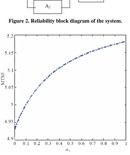
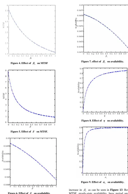
from Figure11 the busy period increases as increase. Similar results can be observed in Figures4, 7, 13 and
15 with respect to where
4.4. Profit Analysis 1.
In these figures, MTSF, availability and profit de- crease as 1 increases while busy period increase with
The system/units are subjected to corrective maintenance at failure as can be observed in states 1-8. From Figure1, the repairman is busy performing corrective maintenance action to the units/system at failure in states 1-8. Ac- cording to [8,9], the expected profit per unit time in- curred to the system in the steady-state is given by: Profit = total revenue generated – cost incurred for repairing the failed units.
A1
A2
[image:5.595.314.531.197.457.2]B
Figure 2. Reliability block diagram of the system.
0 1
PFC A C B (8)
where PF2: is the profit incurred to the system, C0: is the
revenue per unit up time of the system, C1: is the cost per
unit time which the system is under repair.
5. Results and Discussions
In this section, we numerically obtained the results for mean time to system failure, system availability, busy period and profit function for all the developed models. For the model analysis, the following set of parameters values are fixed throughout the simulations for consis-tency: 1 = 0.05, 2 = 0.2, 1 = 0.5, 2 = 0.01,
= 0.1, = 0.5 in Figures 3-7 and assumed 2 =
0.7, in Figures8-17, C0 = 900,000, C1 = 100,000 in
Fig-ures14-17.
Effect of on MTSF, steady-state availability, busy period and profit can be observed in Figures5, 6, 11 and
16. From Figures5, 6 and 16, it is evident that the MTSF,
availability and profit decrease as increases while Figure 3. Effect of 1on MTSF.
4 2 2 3 2 3 4 3 3 2 3 2 2 3 4 2 2 3 3 2 2 4 2 3 4 3 2 3
3 1 2 1 2 1 2 1 2 1 2 1 2 1 2 1 2 1 2 1 2
2 3 3 2 3 3 3 2 3 2 3 3 3 2 3 2 2 2 2 2 2 2
1 2 1 2 2 1 2 1 1 2 2 1 2 1 2 1 2 1 2 1 2 1 2
2 2 2 2 2 3
1 2 1 1 2
2
2 2 4
2 3
N
2 2 3 2 3 2 2 4 2 3 2 2 3 3 3 3
1 1 2 1 2 1 1 2 1 2 1 1 2 1 2 2
4 2 3 2 2 2 3 2 3 2 2 2 4 3 3 4 2 4 2
1 2 1 2 2 1 2 1 2 1 2 1 2 1 1 2 1 1 2 2
4 2 3 3 3 3 2 3 2 2
1 2 2 1 2 2 1 2 1 1 2 2 1
3 3 4
2 2 3 3 2
2 2 2
4 2 2 2 3 2 2 2 2
2 1 1 2 1 1 2 1 1 2 1
3 2 3 4 4 3 3 2 3 2 3 2 2 2 2 3 2
1 2 1 2 1 2 1 2 1 2 1 2 1 2 1 2 1 2 1 2 1 2 1 2 1 2 2
2 2 2 2 2 2 2 2 2 4 3 2 3
1 2 2 1 2 1 1 2 1 2 1 2 2 1 2 2 1
4 2 2
2 2
2 2 5 3
2 2 2 2
2 1 1 2 2
2 2 2 3 2 3 2 2 2 3 3 2 4
1 2 1 1 2 2 1 2 1 2 1 2 1 2 1 2 1 1 2 1 1 2 1
3 2 3 2 3 2 3 2 3 3 2 2 3 2 2
1 2 1 1 2 1 2 1 2 1 2 1 2 2 1 2 1 2 1 2 2 1 2 1
2 3 2
1 2 2
2
2 2 4 5
2 3 2 2
2
2 3 2 4 2 3 2 2 3 3 3 3 2 3 2 2 4
1 2 1 1 2 2 1 2 2 1 2 2 1 2 1 1 2 1 1 2 1
3 3 2 2 3 2 2 3 2 2 3 2 2 3 3 3 2 3 2 3 2 3
1 2 2 1 2 2 1 1 2 1 2 2 1 2 1 1 2 1 1 2 1 2 1 2 1 2 1
2 3 2 3
1 2 1 2 1 2 1 2 1
2 2
2 2 2 2
2
2 3 2 2 2 3 3 2 2 3 2 2 2 3 2
2 1 2 1 2 2 1 2 2 2 2 1 2 1 2 1
4 2 3 2 2 3 2 2 2 3 2 2 3 2 3 2 2 3 2 2 3 2 2
1 2 2 1 1 2 1 2 2 1 2 2 1 2 2 1 2 1 2 2 1 2 1
2 2 2 2 2 2 2 2 2 2 2
1 2 2 1 2 2 1 2 2 1 2 1 2
2 3
3 2 3 2
2 2 4 2
2 2 2 2 2 2 2 2
1 2 1 2 1 2 1 2 1 2 1 2
2 2 2 3 3 2 4 2 2 3 3 2 3 3 2 4 2 2 2 4 2
1 2 1 2 1 2 1 2 1 2 2 1 2 1 1 2
2 2 2
2
2
β1
Figure 4. Effect of 1 on MTSF
Figure 5. Effect of on MTSF.
[image:6.595.72.510.72.733.2]
[image:6.595.329.516.75.730.2]Figure 6. Effect of on availability.
Figure 7. effect of 1 on availability.
η
Figure 8. Effect of on availability.
Figure 9. Effect of 1 on availability.
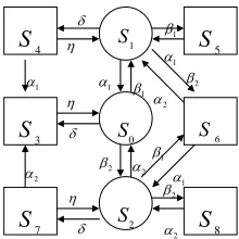
increase in 1 as can be seen in Figure 13. Results of
η
Figure 10. Effect of on busy period.
[image:7.595.75.281.78.646.2]Figure 11. Effect of on busy period.
Figure 12. Effect of 1 on busy period.
with respect to 1 are given in Figures3, 9, 12 and 14.
It is evident from Figures 3, 9 and 14 that as 1
in-creases, the MTSF, availability and profit also increases while busy period decreases as 1increases in Figure12.
Furthermore, the impact of on availability, busy pe-riod and profit can be seen in Figures8, 10 and 17. From
Figures 8 and 17, availability and profit increase as increases and from Figure10 the busy period decreases as increases.
6. Conclusion
In this paper, we constructed a repairable system with two subsystems A and B in series. Subsystem A has two units A1 and A2 in active parallel while subsystem B is a
single unit. We have developed the explicit expressions for the MTSF, availability, busy period and profit func-tion. We performed a parametric investigation of various system parameters on MTSF, system availability and profit function and captured their effects on MTSF, avail-ability, busy period and profit function. This is the main contribution of the paper.
REFERENCES
[1] K. M. El-Said and M. S. EL-Sherbeny, “Evaluation of Reliability and Availability Characteristics of Two Dif- ferent Systems by Using Linear First Order Differential Equations,” Journal of Mathematics and Statistics, Vol. 1, No. 2, 2005, pp. 119-123.
http://dx.doi.org/10.3844/jmssp.2005.119.123
[2] I. Yusuf and N. Hussaini, “Evaluation of Reliability and Availability Characteristics of 2-Out of -3 Standby Sys- tem under a Perfect Repair Condition,” American Journal of Mathematics and Statistics, Vol. 2, No. 5, 2012, pp. 114-119. http://dx.doi.org/10.5923/j.ajms.20120205.03
[3] S. V. Amari, J. B. Dugan and R. B. Misra, “Optimal Re- liability of Systems Subject to Imperfect Fault-Cove- rage,” IEEE Transactions on Reliability, Vol. 48, No. 3, 1999, pp. 275-284. http://dx.doi.org/10.1109/24.799899
[4] K.-H. Wang and B. D. Sivazlian, “Reliability of System with Warm Standbys and Repairmen,” Microelectronics and Reliability,Vol.29, No. 5, 1989, pp. 849-860.
http://dx.doi.org/10.1016/0026-2714(89)90184-4
[5] J.-C. Ke and K.-H. Wang, “The Reliability Analysis of Balking and Reneging in a Repairable System with Warm Standbys,” Quality and Reliability Engineering Interna- tional, Vol. 18, No. 6, 2002, pp. 467-478.
http://dx.doi.org/10.1002/qre.495
[6] K.-H. Wang and J.-C. Ke, “Probabilistic Analysis of a Repairable System with Warm Standbys Plus Balking and Reneging,” Applied Mathematical Modeling, Vol. 27, No. 4, 2003, pp. 327-336.
http://dx.doi.org/10.1016/S0307-904X(02)00133-6
[7] K.-H. Wang, Y.-J. Lai and J.-B. Ke, “Reliability and Sen- sitivity Analysis of a System with Warm Standbys and a Repairable Service Station,” International Journal of Operations Research, Vol. 1, No.1, 2004, pp. 61-70 [8] K. M. El-Said, “Cost Analysis of a System with
Preven-tive Maintenance by Using Kolmogorov’s forward Equa-tions Method”. American Journal of Applied Sciences, Vol.5, No.4, 2008, 405-410.
Common Cause Failures and Preventive Maintenance”. Journal of Mathematics and Statistics, Vol. 5, No.4, 2009. pp 305-310.
http://dx.doi.org/10.3844/jmssp.2009.305.310
[10] M. Y. Haggag, “Cost Analysis of k-Out-of-n Repairable