Stability Analysis of Bubonic Plague Model with the Causing Pathogen Yersinia pestis in the Environment

(1)

http://dx.doi.org/10.4236/aid.2016.63016

How to cite this paper: Ngeleja, R.C., Luboobi, L. and Nkansah-Gyekye, Y. (2016) Stability Analysis of Bubonic Plague Model with the Causing Pathogen Yersinia pestis in the Environment. Advances in Infectious Diseases, 6, 120-137.

http://dx.doi.org/10.4236/aid.2016.63016

Stability Analysis of Bubonic Plague Model

with the Causing Pathogen Yersinia pestis in

the Environment

Rigobert Charles Ngeleja

1*

, Livingstone Luboobi

2

, Yaw Nkansah-Gyekye

1

1_{School of Computational and Communication Science and Engineering, Nelson Mandela African Institution of}

Science and Technology, Arusha, Tanzania

2_{Department of Mathematics, Makerere University, Kampala, Uganda}

Received 23 June 2016; accepted 13 September 2016; published 16 September 2016

This work is licensed under the Creative Commons Attribution International License (CC BY).

http://creativecommons.org/licenses/by/4.0/

Abstract

Bubonic plague is a serious bacterial disease, mainly transmitted to human beings and rodents through flea bite. However, the disease may also be transmitted upon the interaction with the in-fected materials or surfaces in the environment. In this study, a deterministic model for bubonic plague disease with Yersinia pestis in the environment is developed and analyzed. Conditions for ex-istence and stability of the equilibrium points are established. Using Jacobian method disease free equilibrium (DFE) point, E0_{was proved to be locally asymptotically stable. The Metzler matrix} me-thod was used to prove that the DFE was globally asymptotically stable when R0 < 1. By applying Lyapunov stability theory and La Salles invariant principle, we prove that the endemic equilibrium point of system is globally asymptotically stable when R0 > 1. Numerical simulations are done to ve-rify the analytical predictions. The results show that bubonic plague can effectively be controlled or even be eradicated if efforts are made to ensure that there are effective and timely control strategies.

Keywords

Disease Free Equilibrium, Endemic Equilibrium Stability Analysis, Bubonic Plague, Pathogens in the Environment

1. Introduction

Bubonic plague is the bacterial infection caused by Yersinia pestis when the bacteria infect lymphatic system [1].

(2)

It is characterised by geographical foci and extraordinarily adaptation capability which gives it ability to re- emerge even after decades of silence. Thus even though the disease is historic it still infect and kill thousands of people around the world [2].

The disease mainly affects wild rodents, it can also be transmitted to human and other domestic animals through flea bites. Bubonic plague causes fever and very throbbing swelling of the lymph glands also called bu-boes, which is the reason why the disease is called bubonic plague.

When the flea is infested with pathogens causing bubonic plague the bacteria multiply in the proventriculus (foregut) of the flea [3]. The bacteria have the tendency of blocking the flea’s bloodsucking apparatus which consequently lead to inability of flea to pump blood into the midgut for digestion. This makes the flea to become ravenous as a result flea bites the host repetitively while vomiting the bacteria causing disease into the host. When a host dies, fleas move off the body to seek another live warm-blooded host [4].

Although it is not yet clearly known how, but Yersinia pestis may survive in the soil and remain viable and fully virulent for 40 weeks in soil and can cause the infection upon the adequate interaction with the susceptible individual. This is believed to be the reason for possible mechanism of interepizootic persistence, epizootic spread, and as a factor defining plague foci [5].

In this paper, we discuss the stability analysis of the bubonic plague epidemic model in human, rodent and flea population. The model includes the transmission from the environment to the susceptible human or rodent. We also discuss the disease-free equilibrium point, endemic equilibrium point of the model and analyze the local and global stability of these steady states. We finally use the numerical simulation to support our analytical re-sults.

2. Model Formulation

This paper presents the stability analysis of the bubonic plague epidemic model developed by [6]. The model in-cludes four interacting population which are: human population, Flea population, Rodent population and patho-gens in the environment is developed. We use S_H, E_H, I_H and R_H to represent Susceptible human beings, Exposed human beings, Infected human beings and Recovered human beings respectively; S_R, E_R and I_R

for Susceptible rodents, Exposed rodents and Infected rodents respectively. The Susceptible and the Infectious flea are denoted by S_F and I_F respectively. The pathogens in the environment are denoted by A. The total population for human being, rodent and flea population is by

1 H H H H

N =S +E +I +R (1a)

2 F F

N =S +I (1b)

3 R R R

N =S +E +I (1c)

The parameters used in the model are described in Table 1.

Model Equations for Bubonic Plague

Since we allow the population in and out of the compartments, the rate at which new infections occur in a popu-lation will depend on the fraction of the popupopu-lation that is infected (disease prevalence). The infection rate in human depends on the probability that a contact between infectious flea and susceptible human and between in-fectious environment and susceptible human leads to infection. For the rodent the infection depends on the probability that a contact between infectious flea and susceptible rodent and between infectious environment and susceptible rodent leads to infection. For the flea the infection depends on the probability that a contact between infectious human and susceptible flea and between infectious rodent and susceptible flea leads to infection. Therefore the infection rates of susceptible humans, rodent population and flea population are as given in (2a), (2b) and (2c) respectively.

1 2 F fh

I A

N

ω

Γ + (2a)

2 2 F fr

I

A

N

ω

(3)

[image:3.595.172.502.97.719.2]

Table 1.Parameters and their description.

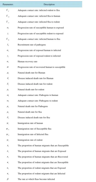
Parameters Description

rf

Γ Adequate contact rate: infected rodent to flea

fh

Γ Adequate contact rate: infected flea to human

fr

Γ Adequate contact rate: infected flea to rodent

1

α Progression rate of susceptible human to exposed

1

γ Progression rate of susceptible rodent to exposed

hf

Γ Adequate contact rate: infected human to flea

4

λ Recruitment rate of pathogens

2

α Progression rate of exposed human to infected

2

γ Progression rate of exposed rodent to infected

3

α Human recovery rate

ϖ Progression rate of recovered human to susceptible

1

µ Natural death rate for Human

1

δ Disease induced death rate for Human

3

δ Disease induced death rate for rodent

3

µ Natural death rate for rodent

1

ω Adequate contact rate: Pathogens to human

2

ω Adequate contact rate: Pathogens to rodent

4

µ Natural death rate for Pathogens

2

µ Natural death rate for flea

2

δ Disease induced death rate for flea

1

ψ Immigration rate of human

2s

ψ Immigration rate of Susceptible flea

2i

ψ Immigration rate of Infected flea

3

ψ Immigration rate of rodent

1

π The proportion of human migrants that are Susceptible

2

π The proportion of human migrants that are Exposed

3

π The proportion of human migrants that are Recovered

1

κ The proportion of rodent migrants that are Susceptible

2

κ The proportion of rodent migrants that are Exposed

3

κ The proportion of rodent migrants that are Infected

(4)

(

)

1 3

1

H r

hf rf

I I

N N

ρ

Γ + −

ρ

Γ (2c)

Pathogens in the environment are recruited at a constant rate λ₄ and they are removed through natural death

4

µ or removed when they contact with susceptible human and rodent at the rates ω₁ and ω₂ respectively. Using the definition of variables and parameters stated in Table 1, we drive model for the dynamics of bu-bonic plague disease in human, rodent, flea and pathogens in the environment as given in (3), (4), (5) and (6) respectively.

Human

1 1 1 1 1

2 d

, d

H F

H fh H H

S I

R A S S

t

π ψ ϖ

α

N

ω

µ

 

= + − _Γ + _ −

  (3a)

2 1 1 1 2 1

2

d

, d

H F

fh H H H

E I

A S E E

t π ψ α N ω α µ

 

= + _Γ + _ − −

  (3b)

(

)

2 3 1 1

d

, d

H

H H H

I

E I I

t =α −α − µ δ+ (3c)

3 1 3 1

d

. d

H

H H H

R

I R R

t =π ψ +α −ϖ −µ (3d)

Rodent

1 3 1 2 3

2 d

d

R F

fr R R

S I

A S S

t

κ ψ

γ

N

ω

µ

 

= − _Γ + _ −

  (4a)

2 3 1 2 2 3

2 d

d

R F

fr R R R

E I

A S E E

t

κ ψ

γ

N

ω

γ

µ

 

= + _Γ + _ − −

  (4b)

(

)

3 3 2 3 3

d d

R

R R

I

E I

t =κ ψ +γ − µ +δ (4c)

Flea

(

)

2 2

1 3

d

1 d

F H R

s hf rf F F

S I I

S S

t

ψ

β ρ

N

ρ

N

µ

 

= − _ Γ + − Γ _ −

  (5a)

(

)

(

)

2 2 2

1 3

d

1 d

F H R

i hf rf F F

I I I

S I

t

ψ

β ρ

N

ρ

N

µ

δ

 

= + _ Γ + − Γ _ − +

  (5b)

where ψ₂_s <ψ₂_i Pathogens

4 1 2 4

d

d H R

A

AS AS A

t =λ −ω −ω −µ (6)

3. Steady State and Local Stability of the Critical Points

In this section we consider existence of equilibrium states and stability of the equilibrium states of the system (3)-(6).

3.1. Disease Free Equilibrium

The model has disease free equilibrium which is obtained by setting IH =EH =RH =0, IR =ER =0, IF =0

(5)

Then we have the disease free-equilibrium point given as 0 1 1 1

, 0, 0, 0 H

E

π ψ

µ

 

=  

 ,

0 1 3

3 , 0, 0 R

E

κ ψ

µ

  =    , 0 2 2 , 0 s F E

ψ

µ

  =  

  and

0

0 A

E = for Human, Rodent, Flea and Pathogen respectively.

Then the disease free equilibrium of the entire system is

(

)

0 0 0 0 0 0 0 0 0 0 0 1 1 1 3 2

1 3 2

, , , , , , , , , , 0, 0, 0, , 0, 0, s , 0, 0

H H H H R R R F F

E S E I R S E I S I A

π ψ

κ ψ

ψ

µ

 

=  

 

3.2. Local Stability of the Disease-Free Equilibrium Point

In this section we consider the local stability analysis of the disease free equilibrium point of the bubonic plague disease system (3)-(6). We analyze the local stability of the disease free equilibrium point using the Jacobian method in which all equations in system (3)-(6) are considered and analyzed at the disease free equilibrium 0

E . In this method we compute and examine the eigenvalues of Jacobian matrix of the system (3)-(6) to prove that the DFE is locally and asymptotically stable. We are required to show that all real parts of the eigenvalues at

0

E are negative. Now in order to attest that the eigenvalues are negative we need to prove the general condition that the determinant and the trace of the Jacobian matrix are positive and negative respectively [7].

Now the Jacobian matrix of the system (3)-(6) at 0

E is given by:

( )

1 1 1 1

1 3

1

1 1 1 1

7 3

1

2 6

3 9

1 1 3 2 0

3 4

3

1 1 3 2

10 4

3

2 11

1 2 2

1 2 8

5

0 0 0 0 0 0

0 0 0 0 0 0 0

0 0 0 0 0 0 0 0

0 0 0 0 0 0 0

0 0 0 0 0 0 0 0

0 0 0 0 0 0 0

0 0 0 0 0 0 0 0 0

k k k k k k E k k k k k

k k k

k α π ψ ω

µ ϖ

µ α π ψ ω

µ α

α

γ κ ψ ω µ

µ γ κ ψ ω

µ γ µ −  − −    −    −  −   ₋ − −  =    −   ₋   − − −  −  −  J                      _ (7) where

(

)

2 1 2 3 1 1 1 2

1 2 3

1 1 2 1 3 2 1 2

1 1 3 2

4 5 1 2 4 6 3 1 1

3 2

7 2 1 8 2 2 9 1

10 2 3 11 3 3

1

hf s rf s fh

s

fr

s

k k k

k k

βρ ψ µ β ρ ψ µ α π ψ µ

π ψ µ κ ψ µ µψ

γ κ ψ µ

ω ω µ α µ δ

µ ψ

α µ µ δ ϖ µ

γ µ µ δ

Γ − Γ Γ

= = =

Γ

= = + + = + +

= + = + = +

= + = +

We now use Trace and determinant method to check the stability of the disease free equilibrium point 0 E in which we need to prove that the trace and the determinant of matrix (7) are negative and positive respectively

Then using mathematica software we prove that trace of the matrix (7) given by

(

)

(

)

(

) (

)

(

)

1 2 1 k6 1 3 2 3 3 3 2 2 2 k5

µ α µ ϖ µ µ γ µ µ δ µ µ δ

= − − + − − + − − + − + − − + −

(6)

where

5 1 2 4, 6 3 1 1

k =ω ω+ +µ k =α +µ δ+

It is clear that the trace of the matrix (7) in negative. Then using the same software (mathematica) we are able to prove that the determinant of the matrix (7) is positive provided:

(

2 2

)

(

2 13 2

)(

(

3 3

)

) (

2 1

)(

2 13 1 1

)

1

rf fr hf fh

γ γ ρ ρα α

β

µ δ µ γ µ δ α µ α µ δ

 Γ Γ − Γ Γ 

+ <

 

+ _ + + + + + _

where

(

2 2

)

(

2 13 2

)(

(

3 3

)

) (

2 12

)(

13 1 1

)

1

rf fr hf fh

γ γ ρ ρα α

β

µ δ µ γ µ δ α µ α µ δ

 Γ Γ − Γ Γ 

+

 

+ _ + + + + + _ (8)

is the basic reproduction number, R₀.

0

R measures the average number of secondary infection produced when a typical infectious individual enters an entirely susceptible population. In our case, due to presence of multiple transmission cycle the basic repro-ductive number do not give the number of cases infected by a single individual but rather the geometric mean of the number of infections per generation [8].

Referring to (8), the geometric mean of the number of infections per generation depends on: rodent’s infective

period

3 3

1

µ δ

+ , the probability that flea gets the disease from the rodent or human which are

(

1−ρ

)

Γrf or

hf

ρΓ respectively The human infective period

1 1 3

1

µ δ α

+ + , probability that human survive the infected class

2

1 2

α

µ α

+ , the rate at which fleas gets infected β, flea’s infective period 2 2 1

µ

+

δ

, probability that rodent

sur-vive the infected class 2

3 2

γ

µ

+

γ

, the adequate contact rate flea to human Γfh, the adequate contact rate flea to rodent Γ_fr and the rate at which human and rodent become exposed to the the disease which are α₁ and γ₁ respectively.

Thus disease free equilibrium point 0

E is therefore locally asymptotically stable and leads to the following theorem:

Theorem 1. The Disease Free Equilibrium 0

E of bubonic plague is locally asymptotically stable if R₀<1 and unstable if R₀ >1.

3.3. Global Stability of the Disease-Free Equilibrium Point

In this section we analyze the global stability of the disease free equilibrium point using Metzler matrix method as stated by [9]. To do this we first sub-divide the general system (3)-(6) of bubonic plague disease into trans-mitting and non-transtrans-mitting component.

Now let Y_n be the vector for non-transmitting compartment, Y_i be the vector for transmitting compartment and

0,

E n

Y be the vector of disease free point. Then

(

0

)

1 , 2

3

d d d

d n

n E n i

i i

t

 ₌ ₋ ₊

   ₌ 

Y

A Y Y A Y

Y A Y

(9)

We then have

(

)

T

(

)

₀ ₁ ₁ ₁ ₃ ₂

,

1 3 2

, , , , , , , , , 0, , s

n SH RH SR SF i EH IH ER IR IF A E n

κ ψ ψ

π ψ

µ

 

= = _{= } _

 

(7)

0

1 1

1

, 1 3

3

2

2 H

H

n E n R s F S R S S π ψ µ κ ψ µ ψ µ  ₋          − _{= } _ −      ₋      Y Y

Now to prove the global stability of the DFE we need to show that Matrix A₁ has real negative eigenvalues and A₃ is a Metzler matrix in which all off diagonal element must be non-negative. Referring to (9) we write the general model as given below

1 1

1

1 1 1 1

3 1 3 1

1 1 3 2

1 3 1 3

3 2 2 2 2 , . H H

H H H H

H

H H H R

R

R R R

s F F F

s F

S E

R kS S I

R

I R R E

S

MS S I

YS S I

S A

π ψ µ

π ψ ϖ α µ

π ψ α ϖ µ

κ ψ

κ ψ γ µ _µ

ψ β µ

ψ µ  ₋          + − −   _ _ _ _  ₊ ₋ ₋  _ _    _{ =} ₊ _ _    − −  _ − _ _ _   _ _ − −     _ _  ₋          A A and

(

)

(

)

(

)

2 1 1 2 1

2 3 1 1

2 3 1 2 3

3

3 3 2 3 3

2 2 2

4 1 2 4

, ,

H H H H

R R R R

R R R

i F F F

H R

kS E E E

E I I I

MS E E E

E I I

YS I I

AS AS A A

π ψ α α µ

α α µ δ

κ ψ γ γ µ

κ ψ γ µ δ

ψ β µ δ

λ ω ω µ

+ − −      ₋ ₋ ₊         + − −    =  ₊ ₋ ₊         ₊ ₋ ₊      _ _  ₋ ₋ ₋  _ _   A For

(

)

1 2

2 2 1 3

1

F F H R

fh fr hf rf

I I I I

k A M A Y

N

ω

N

ω

ρ

N

ρ

N

 

   

= Γ_ + _ = Γ_ + _ =_ Γ + − Γ _

     

Now using the transmitting and non-transmitting element on the general system we will have the matrices be-low:

(

)

1 1 1 3 2 0 0

0 0 0

µ ϖ ϖ µ µ µ −    ₋ ₊    =  −    −  

A (10)

(

)

1 1 1 2 1 1 1 1

1 2 1

3

1 1 3 2

2 1 1 3 2

3 2 3

2 1 2 3

2 1 1 2 1 3

0 0 0 0

0 0 0 0 0

0 0 0 0

1

0 0 0 0

fh

s

fr

s

s hf s rf

α π ψ µ α π ψ ω

µψ µ

α

γ κ ψ µ γ κ ψ ω

µ ψ µ

βψ µ ρ βψ µ ρ

µ π ψ µ κ ψ

− Γ  −          − Γ = −     

 − Γ − − Γ 

 

 

(8)

(

)

(

)

(

)

(

)

₍

₎

1 1 1 2 1 1 1 1

2 1

1 2 1

2 1

1 1 3 2 1 1 3 2

2 3

3 2 3

3

2 3 3

2 3

3 2 2

1 3 2

2

0 0 0

0 0 0 0

0 0 0

0 0 0 0

1

0 0 0

0 0 0 0 0

fh

s

fr

s

rf s

α π ψ µ α π ψ ω

α µ

µψ µ

α ζ

γ κ ψ µ γ κ ψ ω

γ µ

µ ψ µ

γ µ δ

β ρ ψ µ

ζ µ δ

κ ψ µ

ζ Γ

 

− +

 

 ₋ 

 

Γ

 ₋ ₊ 

 

=  

 − + 

 

− Γ

 ₋ ₊ 

 

 ₋ 

 

A (12)

where ζ₁=

(

α₃+µ δ₁+ ₁

)

, ζ₂=

(

ω₁S_H +ω₂S_R+µ₄

)

and ₃ 2 1

1 1 2

.

hf s

βρ ψ µ ζ

π ψ µ Γ =

Now when we consider matrix A₁, the computation shows that the eigenvalues are real and negative, which now confirms that the system

(

0

)

1 , 2

d d

n

n E n i

t = − +

Y

A Y Y A Y

is globally and asymptotically stable at

0

E

Y . And for matrix A₃ we find that all its off-diagonal elements are non-negative and thus A₃ is a Metzler stable matrix.Therefore Disease Free Equilibrium point for the general bubonic plague system is globally asymptotically stable as a result we have the following theorem:

Theorem 2. The disease-free equilibrium point is globally asymptotically stable in E₀ if R₀ <1 and un- stable if R₀ >1.

3.4. Existence of Endemic Equilibrium

Here we consider the situation in which the disease persist in a population. We investigate conditions for exis-tence of the endemic equilibrium point of the system (3)-(6). The endemic equilibrium point

(

)

* * * * * * * * * * *

, , , , , , , , ,

H H H H R R R F F

E S E I R S E I S I A is obtained by solving the equations obtained by setting the deriva-tives of (3)-(6) equal to zero as in (13)-(16) which exist for R₀ >1.

Human

1 1 1 1 1

2

0 F

H fh H H

I

R A S S

N

π ψ ϖ

+ −

α

_Γ +

ω

_ −

µ

=

  (13a)

2 1 1 1 2 1

2

0 F

fh H H H

I

A S E E

N

π ψ α

+ _Γ +

ω

_ −

α

−

µ

=

  (13b)

(

)

2EH 3IH 1 1 IH 0

α −α − µ δ+ = (13c)

3 1 3IH RH 1RH 0

π ψ +α −ϖ −µ = (13d)

Rodent

1 3 1 2 3

2

0 F

fr R R

I

A S S

N

κ ψ

−

γ

_Γ +

ω

_ −

µ

=

  (14a)

2 3 1 2 2 3

2

0 F

fr R R R

I

A S E E

N

κ ψ

+

γ

_Γ +

ω

_ −

γ

−

µ

=

  (14b)

(

)

3 3 2ER 3 3 IR 0

κ ψ +γ − µ +δ = (14c)

(9)

(

)

2 2

1 3

1 0

H R

s hf rf F F

I I

S S

N N

ψ

−

β ρ

_ Γ + −

ρ

Γ _ −

µ

=

  (15a)

(

)

(

)

2 2 2

1 3

1 0

H R

i hf rf F F

I I

S I

N N

ψ

+

β ρ

_ Γ + −

ρ

Γ _ −

µ

+

δ

=

  (15b)

4 1ASH 2ASR 4A 0

λ ω− −ω −µ = (16)

Since it is difficult to obtain explicitly the endemic equilibrium points of the model we will prove its existence using the study by [10] [11]. For the endemic equilibrium to exist it must satisfy the condition EH ≠0 or

0 H

I ≠ or ER≠0 or IR≠0 or IF ≠0 or A≠0 that is SH >0 or EH >0 or IH >0 or SR >0 or 0

R

I > or ER >0 or SF >0 or IF >0 or A>0 must be satisfied. Now adding system (13)-(16) we have

(

)

(

)

(

)

1 2 2 3 4 1 2

3 1 2 3 1 2 4 0

s i H H H H F F

R R R H F R H R

S E I R S I

S E I I I I AS AS A

ψ ψ

ψ

λ

µ

δ

ω

µ

+ + + + − + + + − +

− + + − − − − − − = (17)

Substituting N₁=S_H+E_H+I_H +R_H, N₂=S_F+I_F and N₃ =S_R+E_R +I_R in (17) we have

1 2s 2i 3 1N1 2N2 3N3 1IH 2IF 3IR 4 1ASH 2ASR 4A 0

ψ ψ+ +ψ +ψ −µ −µ −µ −δ −δ −δ +λ ω− −ω −µ = (18)

But from Equation (16), we have λ ω₄− ₁ASH−ω₂ASR−µ₄A=0

It follows that

1N1 2N2 3N3 1IH 2IF 3IR = 1 2s 2i 3

µ +µ +µ +δ +δ +δ ψ ψ+ +ψ +ψ

Since ψ ψ₁+ ₂s+ψ₂i+ψ₃>0, µ >1 0, µ >2 0, µ >3 0, δ >1 0, δ >2 0 and δ >3 0 we can discern that 1N1 0

µ > , µ₂N₂>0, µ₃N₃>0, δ₁IH >0, δ2IF >0 and δ3IR >0 implying that SH >0, EH >0, IH >0, 0

F

S > , IF >0, SR >0, ER >0 and IR >0.

Hence endemic equilibrium point of the bubonic plague disease model in human, rodent, flea and pathogens in the environment exists.

Since the endemic equilibrium points exist, we now determine the conditions under which they are stable or unstable. We prove whether the solution starting sufficiently close to the equilibrium remains close to the equi-librium and approaches the equiequi-librium as t→ ∞, or if there are solutions starting arbitrary close to the equili-brium which do not approach it respectively.

3.5. Global Stability of Endemic Equilibrium Point

Using the idea from the study by [12] we say that the local stability of the Disease Free Equilibrium advocates for local stability of the Endemic Equilibrium for the reverse condition. We then work to find the global stability of Endemic equilibrium using a Korobeinikov approach as stipulated in [12]-[14] by forming a suitable Lyapu-nov function for our general model as given below:

We construct the Lyapunov function as given in the form:

(

*

)

ln

i i i i

V =

∑

a y −y y

where a_i is defined as a properly selected positive constant, y_i defines the population of the th

i compart-ment, and *

i

y is the equilibrium point.

We will have the following Lyapunov function,

(

)

(

)

(

)

(

)

(

)

(

)

(

)

(

)

(

)

(

)

* * *

1 2 3

* * *

4 5 6

* * *

7 8 9

* 10

ln ln ln

ln

H H H H H H H H H

H H H R R R R R R

R R R F F F F F F

V W S S S W E E E W I I I

W R R R W S S S W E E E

W I I I W S S S W I I I

W A A A

= − + − + −

+ − + − + −

(10)

The constants W_i are non negative in Φ such that Wi >0 for i=1, 2, 3,,10. The Lyapunov function V

together with its constants W W₁, ₂,,W₁₀ chosen in such way that V is continuous and differentiable in a space We then compute the time derivative of V from it we get;

* * * * *

1 2 3 4 5

* * * *

6 7 8 9 10

d d d d d

d

1 1 1 1 1

d d d d d d

d d d d

1 1 1 1 1

d d d d

H H H H H H H H R R

H H H H R

R R R R F F F F

R R F F

S S E E I I R R S S

V

W W W W W

t S t E t I t R t S t

E E I I S S I I A

W W W W W

E t I t S t I t

          = _ − _ + _ − _ + _ − _ + _ − _ + _ − _                   + _ − _ + _ − _ + _ − _ + _ − _ + −         * d d A A t      

Now using the general system (3)-(6) we will have

(

)

[

]

*

1 1 1 1 1 1

2

*

2 2 1 1 1 2 1

2

*

3 2 3 1 1

*

4 3 1 3 1

* 5 d 1 d 1 1 1 1 H F

H fh H H

H

H F

fh H H H

H

H H H

H

H H H

H

R

S I

V

W R A S S

t S N

E I

W A S E E

E N

I

W E I I

I

R

W I R R

R

S W

S

π ψ ϖ α ω µ

π ψ α ω α µ

α α µ δ

π ψ α ϖ µ

 

   

= _ − __ + − _Γ + _ − _

 

   

 

   

+ _ − __ + _Γ + _ − − _

        + _ − _{ } − − + _     + _ − _ + − −   + −

(

)

(

)

1 3 1 2 3

2

*

6 2 3 1 2 2 3

2

*

7 3 3 2 3 3

*

8 2 2

1 3 9 1 1 1 1 F

fr R R

R F

fr R R R

R

R R

R

F H R

s hf rf F F

F

I

A S S

N

E I

W A S E E

E N

I

W E I

I

S I I

W S S

S N N

W

κ ψ γ ω µ

κ ψ γ ω γ µ

κ ψ γ µ δ

ψ β ρ ρ µ

 

   

− Γ + −

                 

+ _ − __ + _Γ + _ − − _

          + _ − _{ } + − + _        

+  −  −  Γ + − Γ  − 

    

+

(

)

(

)

[

]

*

2 2 2

1 3

*

10 4 1 2 4

1 1

1

F H R

i hf rf F F

F

H R

I I I

S I

I N N

A

W AS AS A

A

ψ β ρ ρ µ δ

λ ω ω µ

 

   

−  + Γ + − Γ − + 

   

    

 

+ _ − _ − − −

 

At endemic equilibrium point we have Human

*

* * * *

1 1 1 * 1 1

2

, F

H fh H H

I

R A S S

N

π ψ = −ϖ +α _Γ −ω _ +µ

  (19a)

*

* * * *

2 1 1 * 1 2 1

2

, F

fh H H H

I

A S E E

N

π ψ = −α _Γ −ω _ +α +µ

  (19b)

(

)

(

* *

)

2 * 3 1 1

1

H H

H

I I

E

α

=

α

+

µ δ

+ (19c)

* * *

3 1 3IH RH 1RH

π ψ = −α +ϖ +µ (19d)

(11)

*

* * *

1 3 1 * 2 3

2 F

fr R R

I

A S S

N

κ ψ

=

γ

_Γ −

ω

_ +

µ

  (20a)

*

* * * *

2 3 1 * 2 2 3

2 F

fr R R R

I

A S E E

N

κ ψ

= −

γ

_Γ −

ω

_ +

γ

+

µ

  (20b)

(

)

* *

3 3 2ER 3 3 IR

κ ψ

= −

γ

+

µ δ

+ (20c)

Flea

(

)

* *

2 * * 2

1 3

1

H R

s hf rf F F

I I

S S

N N

ψ

=

β ρ

_ Γ − −

ρ

Γ _ +

µ

  (21a)

(

)

(

)

* *

2 * * 2 2

1 3

1

H R

i hf rf F F

I I

S I

N N

ψ

= −

β ρ

_ Γ − −

ρ

Γ _ +

µ

+

δ

  (21b)

* * * * *

4 1A SH 2A SR 4A

λ =ω +ω +µ (22)

We can then rewrite d d

V

t using (19), (20), (21) and (22) as:

* *

* * * *

1 1 * 1 1 1 1 1

2 2

* *

* * * *

2 1 * 1 2 1 1 1 2 1

2 2 * 3 d 1 d 1 1

H F F

H fh H H H fh H H

H

H F F

fh H H H fh H H H

H

S I I

V

W R A S S R A S S

t S N N

E I I

W A S E E A S E E

E N N

I W

I

ϖ α ω µ ϖ α ω µ

α ω α µ α ω α µ

 

     

=  − − + Γ −  + + − Γ +  − 

 

    

 

     

+  − − Γ −  + + + Γ +  − − 

         + _ − 

(

)

(

)

* *

3 1 1 3 1 1

*

* * *

4 3 1 3 1

* *

* * *

5 1 * 2 3 1 2 3

2 2 * 6 1 1 1 1 1

H H H H H

H

H H H H H H

H

R F F

fr R R fr R R

R

fr R

I I E I I

E

R

W I R R I R R

R

S I I

W A S S A S S

S N N

E W

E

α µ δ α µ δ

α ϖ µ α ϖ µ

γ ω µ γ ω µ

γ    + + − − +           _ _ + _ − _{ }− + + + − − _          

+ _ − __ _Γ − _ + − _Γ + _ − _

 

    

 

+ _ − _ − Γ

 

(

)

(

)

(

)

(

)

*

* * * *

2 2 3 1 2 2 3

*

2 2

*

* *

7 2 3 3 2 3 3

* * *

* *

8 * * 2

1 3

1

1 1 1

F F

R R R fr R R R

R

R R R R

R

F H R H R

hf rf F F hf rf

F

I I

A S E E A S E E

N N

I

W E I E I

I

S I I I I

W S S

S N N N N

ω γ µ γ ω γ µ

γ µ δ γ µ δ

β ρ ρ µ β ρ ρ

     

− + + + Γ + − −

                + _ − _{ }− + + + − + _        

+ _ − _ _ Γ − − Γ _ + − _ Γ + − Γ _

     

(

)

(

)

(

)

(

)

2 * * * *

9 * * 2 2

1 3

2 2

1 3

*

* * * * *

10 1 2 4 1 2 4

1 1

1

F F

F H R

hf rf F F

F

H R

hf rf F F

H R H R

S S

I I I

W S I

I N N

I I

S I

N N

A

W A S A S A AS AS A

A

µ

β ρ ρ µ δ

ω ω µ ω ω µ

  −           

+  − −  Γ − − Γ  + + 

   



 

+ _ Γ + − Γ _ − + _

  

 

 

+ _ − _{ } + + − − − _

(12)

After simplification the above equation becomes:

2 2 2

* * *

1 2 3

2 2 2

* * *

4 5 6

2 2 2

* * *

7 8 9

2 *

10

d

1 1 1

d

1 1 1

1 , , , , , , , ,

H H H

H R R

R F F

H H H H R R R F

S E I

V

W W W

t S E I

R S E

W W W

R S E

I S I

W W W

I S I

A

W F S E I R S E I S

A

     

= − _ − _ − _ − _ − _ − _

     

     

− _ − _ − _ − _ − _ − _

     

     

− _ − _ − _ − _ − _ − _

     

 

− _ − _ +

 

(

IF,A

)

where the function F S

(

_H,E_H,I_H,R_H,S_R,E_R,I_R,S_F,I_F,A

)

is non positive, Now following the procedures by

[15] [16]. We have F S

(

_H,E_H,I_H,R_H,S_R,E_R,I_R,S_F,I_F,A

)

≤0 for all SH,EH,IH,RH,SR,ER,IR,SF,IF,A,

Then d 0

d

V

t ≤ for all SH,EH,IH,RH,SR,ER,IR,SF,IF,A and it is zero when

*

H H

S =S , E_H =E_H* , I_H =I*_H,

*

H H

R =R , *

R R

S =S , *

R R

E =E , *

R R

I =I , *

F F

S =S , *

F F

I =I , *

A=A Hence the largest compact invariant set

in SH,EH,IH,RH,SR,ER,IR,SF,IF,A such that

d 0 d

V

t = is the singleton *

E which is Endemic Equilibrium

point of the model system (3)-(6).

LaSalles’s invariant principle by [17] then implies that E* is globally asymptotically stable in the interior of the region of SH,EH,IH,RH,SR,ER,IR,SF,IF,A and thus leads to the Theorem 3.

Theorem 3. If R₀>1 then the bubonic plague disease model system (3)-(6) has a unique endemic equili- brium point E* which is globally asymptotically stable in SH,EH,IH,RH,SR,ER,IR,SF,IF, .A

4. Numerical Simulation

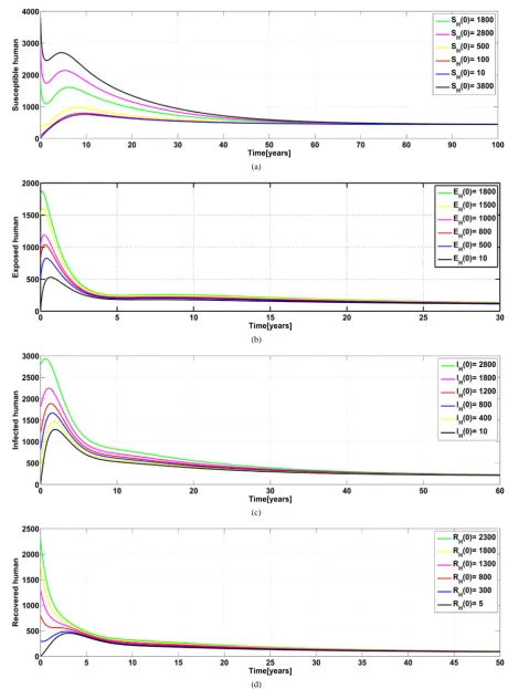
Numerical simulation is carried out in order to observe and understand the kinetics of bubonic plague disease and demonstrate analytical results. In particular we illustrate through numerical simulation the stability of the endemic equilibrium states in human, rodent, flea and pathogens in the environment.

Parameter Values

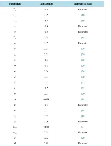
The values of the parameters used in bubonic plague disease model are shown in Table 2. The parameters are taken from the previous studies that relate to this study, existing information and through estimation.

[image:12.595.188.438.102.241.2]

In the simulation we assume different cases where each sub-population starts at different initial values (six different initial values) ultimately returns to its endemic point. We thus justify that a solution that starts suffi-ciently close to the equilibrium remains close to it and it eventually approaches the equilibrium as t→ ∞.

(13)

[image:13.595.142.505.99.578.2]

Table 2.Parameters values for Bubonic Plague disease model.

Parameters Value/Range Reference/Source

rf

Γ 0.6 Estimated

fh

Γ 0.09 [18]

fr

Γ 4.7 [19]

1

α 0.9 Estimated

1

γ 0.9 Estimated

hf

Γ 0.28 [18]

4

λ 0.89 Estimated

2

α 0.04 [20]

2

γ 0.05 [20]

3

α 0.1 [20]

ϖ 0.1 [20]

1

µ 0.04 [20]

1

δ 0.04 [20]

3

δ 0.05 [21]

3

µ 0.2 [22]

1

ω 0.01 [20]

2

ω 0.073 [18]

4

µ 0.1 Estimated

2

µ 0.07 [18]

2

δ 0.03 [18]

1

ψ 0.09 Estimated

2S

ψ 0.008 [21]

2i

ψ 0.08 Estimated

3

ψ 0.03 [20]

β 0.99 Estimated

(14)

(a)

(b)

(c)

[image:14.595.80.541.79.703.2]

(d)

(15)

(a)

(b)

[image:15.595.80.543.80.525.2]

(c)

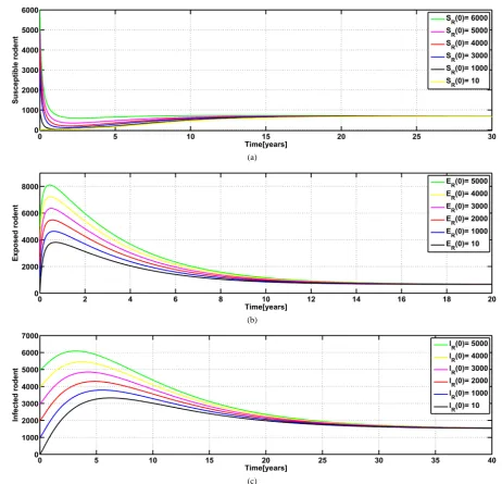
Figure 2.Simulation of the model’s solution trajectories to show stability of the endemic point in subsystem (4).

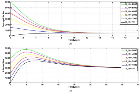
The dynamics in the flea population are as seen in Figure 3, we can see that the number of susceptible flea decreases exponentially as they die naturally or acquire infection from the infected rodent or human at the rate

hf

(16)

(a)

[image:16.595.83.540.83.385.2]

(b)

Figure 3.Simulation of the model’s solution trajectories to show stability of the endemic point of subsystem (5).

Figure 4. Simulation of the model’s solution trajectories to show stability of the endemic point in (6).

5. Conclusion

In this paper, we have considered a bubonic plague in human, rodent and flea with Yersinia pestis in the envi-ronment. We have carried out the stability analysis of the equilibrium states in which the analytical results show that the disease free equilibrium point is locally and globally asymptotically stable when R₀<0 and unstable when R₀>0. This result necessitates that the basic reproduction number, which is the expected number of secondary cases produced by a single infected individual during the entire infectious period of that particular in-dividual in a completely susceptible population is a key non-dimension parameter that dictates whether the dis-ease will spread or die out. When R₀ is increased or decreased above or below unity compels to the persistence or eradication of bubonic plague disease respectively. The decrease or increase of the basic reproduction number

will as a result affects negatively or positively the flea’s infective period

2 2

1

[image:16.595.89.540.413.553.2]

(17)

sur-vive the infected class 2

3 2

γ

µ

+

γ

, the adequate contact rate flea to human Γfh, rodent’s infective period

3 3

1

µ δ

+ , the probability that flea gets the disease from the rodent or human which are

(

1−ρ

)

Γrf or ρΓhf

respectively. The human infective period

1 1 3

1

µ δ α

+ + , probability that human survive the infected class

2

1 2

α

µ α

+ , the rate at which fleas gets infected β, the adequate contact rate flea to rodent Γfr and the rate at which human and rodent become exposed to the the disease which are α₁ and γ₁ respectively. The endemic equilibrium point is also found to be locally and globally asymptotically stable whenever they exist. Using the model’s parameters values from literature reviewed in this paper and some estimated, we use the simulation to show the endemic equilibrium for Human, Rodent, Flea and pathogens in the environment are stable thus sup-ports the analytical results. We observe that without intervention that controls the value of R₀ to less than a unity bubonic plague may be very fatal and a life threatening disease whenever it occurs.

Acknowledgements

We thank the Editor and the referee for their comments. Research of R. C. Ngeleja is funded by The Govern-ment of Tanzania through Nelson Mandela African Institution of Science and Technology (NM-AIST). This support is greatly appreciated.

References

[1] Gonzalez, R.J. and Miller, V.L. (2016) A Deadly Path: Bacterial Spread during Bubonic Plague. Trends in Microbiol-ogy, 24, 239-241. http://dx.doi.org/10.1016/j.tim.2016.01.010

[2] Guinet, F., Avffe, P., Filali, S., Huon, C., Savin, C., Huerre, M., Fiette, L. and Carniel, E. (2015) Dissociation of Tissue Destruction and Bacterial Expansion during Bubonic Plague. PLoS Pathogens, 11, e1005222.

http://dx.doi.org/10.1371/journal.ppat.1005222

[3] Eisen, R.J., Dennis, D.T. and Gage, K.L. (2015) The Role of Early-Phase Transmission in the Spread of Yersinia pestis.

Journal of Medical Entomology, 52, 1183-1192. http://dx.doi.org/10.1093/jme/tjv128

[4] Ayyadurai, S., Houhamdi, L., Lepidi, H., Nappez, C., Raoult, D. and Drancourt, M. (2008) Long-Term Persistence of Virulent Yersinia Pestis in Soil. Microbiology, 154, 2865-2871. http://dx.doi.org/10.1099/mic.0.2007/016154-0 [5] Eisen, R.J., Petersen, J.M., Higgins, C.L., Wong, D., Levy, C.E., Mead, P.S., Schriefer, M.E., Griffth, K.S., Gage, K.L.

and Beard, C.B. (2008) Persistence of Yersinia pestis in Soil under Natural Conditions. Emerging Infectious Diseases,

14, 941. http://dx.doi.org/10.3201/eid1406.080029

[6] Ngeleja, R.C., Luboobi, L.S. and Nkansah-Gyekye, Y. (2016) Modelling the Dynamics of Bubonic Plague with Yersi-nia pestis in the Environment. Communications in Mathematical Biology and Neuroscience, 2016, 5-10.

[7] Martcheva, M. (2015) Introduction to Mathematical Epidemiology. Vol. 61, Springer. http://dx.doi.org/10.1007/978-1-4899-7612-3

[8] Li, J., Blakeley, D. and Smith, R. (2011) The Failure of r0. Computational and Mathematical Methods in Medicine, 2011. Article ID: 527610.

[9] Castillo-Chavez, C., Blower, S., Driessche, P., Kirschner, D. and Yakubu, A.-A. (2002) Mathematical Approaches for Emerging and Reemerging Infectious Diseases: Models, Methods, and Theory. Springer.

http://dx.doi.org/10.1007/978-1-4757-3667-0

[10] Tumwiine, J., Mugisha, J. and Luboobi, L.S. (2007) A Mathematical Model for the Dynamics of Malaria in a Human Host and Mosquito Vector with Temporary Immunity. Applied Mathematics and Computation, 189, 1953-1965. http://dx.doi.org/10.1016/j.amc.2006.12.084

[11] Massawe, L.N., Massawe, E.S. and Makinde, O.D. (2015) Temporal Model for Dengue Disease with Treatment. Ad-vances in Infectious Diseases, 5, 21. http://dx.doi.org/10.4236/aid.2015.51003

[12] Van den Driessche, P. and Watmough, J. (2002) Reproduction Numbers and Sub-Threshold Endemic Equilibria for Compartmental Models of Disease Transmission. Mathematical Biosciences, 180, 29-48.

http://dx.doi.org/10.1016/S0025-5564(02)00108-6

(18)

Medicine and Biology, 21, 75-83. http://dx.doi.org/10.1093/imammb/21.2.75

[14] Korobeinikov, A. (2007) Global Properties of Infectious Disease Models with Nonlinear Incidence. Bulletin of Ma-thematical Biology, 69, 1871-1886. http://dx.doi.org/10.1007/s11538-007-9196-y

[15] McCluskey, C. (2006) Lyapunov Functions for Tuberculosis Models with Fast and Slow Progression. Mathematical Biosciences and Engineering: MBE, 3, 603-614. http://dx.doi.org/10.3934/mbe.2006.3.603

[16] Korobeinikov, A. and Wake, G.C. (2002) Lyapunov Functions and Global Stability for Sir, Sirs, and Sis Epidemiolog-ical Models. Applied Mathematics Letters, 15, 955-960. http://dx.doi.org/10.1016/S0893-9659(02)00069-1

[17] La Salle, J. (1976) The Stability of Dynamical Systems. SIAM.

[18] Benkirane, S., Shankland, C., Norman, R. and McCaig, C. (2009) Modelling the Bubonic Plague in a Prairie Dog Bur-row: A Work in Progress. 8th Workshop on Process Algebra and Stochastically Timed Activities, Edinburgh, 26-27 August 2009, 145-152.

[19] Li, W.-H. (1993) Unbiased Estimation of the Rates of Synonymous and Nonsynonymous Substitution. Journal of Mo-lecular Evolution, 36, 96-99. http://dx.doi.org/10.1007/BF02407308

[20] Keeling, M. and Gilligan, C. (2000) Bubonic Plague: A Metapopulation Model of a Zoonosis. Proceedings of the Roy-al Society of London Series B: Biological Sciences, 267, 2219-2230. http://dx.doi.org/10.1098/rspb.2000.1272 [21] Keeling, M. and Gilligan, C. (2000) Metapopulation Dynamics of Bubonic Plague. Nature, 407, 903-906.

http://dx.doi.org/10.1038/35038073

[22] Galtier, N. and Mouchiroud, D. (1998) Isochore Evolution in Mammals: A Human-Like Ancestral Structure. Genetics,

150, 1577-1584.

[23] Lemon, S.M., Sparling, P.F., Hamburg, M.A., Relman, D.A., Choffnes, E.R., Mack, A., et al. (2008) Vectorborne Dis-eases: Understanding the Environmental, Human Health, and Ecological Connections, Workshop Summary (Forum on Microbial Threats). National Academies Press, Washington DC.

[24] McNeill, W. (2010) Plagues and Peoples. Anchor, Norwell.

[25] Poland, J.D. and Dennis, D.T. (1998) Plague. In: Evans, A.S. and Brachman, P.S., Eds., Bacterial Infections of Hu-mans, Springer, Berlin, 545-558. http://dx.doi.org/10.1007/978-1-4615-5327-4_28

[26] Gage, K.L. and Kosoy, M.Y. (2005) Natural History of Plague: Perspectives from More than a Century of Research.

Annual Review of Entomology, 50, 505-528. http://dx.doi.org/10.1146/annurev.ento.50.071803.130337

[27] Scott, S. and Duncan, C.J. (2001) Biology of Plagues: Evidence from Historical Populations. Cambridge University Press, Cambridge. http://dx.doi.org/10.1017/CBO9780511542527

[28] Dennis, D.T. and Staples, J.E. (2009) Plague. In: Evans, A.S. and Brachman, P.S., Eds., Bacterial Infections of Hu-mans, Springer, Berlin, 597-611. http://dx.doi.org/10.1007/978-0-387-09843-2_28

[29] Davis, S. and Calvet, E. (2005) Fluctuating Rodent Populations and Risk to Humans from Rodent-Borne Zoonoses.

Vector-Borne & Zoonotic Diseases, 5, 305-314. http://dx.doi.org/10.1089/vbz.2005.5.305

[30] Putzker, M., Sauer, H. and Sobe, D. (2000) Plague and Other Human Infections Caused by Yersinia Species. Clinical Laboratory, 47, 453-466.

[31] Samia, N.I., Kausrud, K.L., Heesterbeek, H., Ageyev, V., Begon, M., Chan, K.-S. and Stenseth, N.C. (2011) Dynamics of the Plague-Wildlife-Human System in Central Asia Are Controlled by Two Epidemiological Thresholds. Proceed-ings of the National Academy of Sciencesof the United States of America, 108, 14527-14532.

http://dx.doi.org/10.1073/pnas.1015946108

(19)

Submit or recommend next manuscript to SCIRP and we will provide best service for you:

Accepting pre-submission inquiries through Email, Facebook, LinkedIn, Twitter, etc. A wide selection of journals (inclusive of 9 subjects, more than 200 journals) Providing 24-hour high-quality service

User-friendly online submission system Fair and swift peer-review system

Efficient typesetting and proofreading procedure

Display of the result of downloads and visits, as well as the number of cited articles Maximum dissemination of your research work