Neural Network Approach for Solving Singular Convex
Optimization with Bounded Variables
*
Rendong Ge#, Lijun Liu, Yi Xu
School of Science, Dalian Nationalities University, Dalian, China Email: #[email protected], [email protected], [email protected] Received May 1,2013; revised June 1, 2013; accepted June 8, 2013
Copyright © 2013 Rendong Ge et al. This is an open access article distributed under the Creative Commons Attribution License, which permits unrestricted use, distribution, and reproduction in any medium, provided the original work is properly cited.
ABSTRACT
Although frequently encountered in many practical applications, singular nonlinear optimization has been always rec-ognized as a difficult problem. In the last decades, classical numerical techniques have been proposed to deal with the singular problem. However, the issue of numerical instability and high computational complexity has not found a satis-factory solution so far. In this paper, we consider the singular optimization problem with bounded variables constraint rather than the common unconstraint model. A novel neural network model was proposed for solving the problem of singular convex optimization with bounded variables. Under the assumption of rank one defect, the original difficult problem is transformed into nonsingular constrained optimization problem by enforcing a tensor term. By using the augmented Lagrangian method and the projection technique, it is proven that the proposed continuous model is conver-gent to the solution of the singular optimization problem. Numerical simulation further confirmed the effectiveness of the proposed neural network approach.
Keywords: Neural Networks; Singular Nonlinear Optimization; Stationary Point; Augmented Lagrangian Function; Convergence; LaSalle’s Invariance Principle Plain
1. Introduction
The nonlinear model with rank one defect is of great importance for its singular nature. Follwing works of Schnabel and Dan Feng [1-3], we have made great im- provement for such problem by applying Tensor methods by numerical solution [4,5]. For large-scale computational problems, the computation of the classical numerical method is still far from satisfactory.
In recent years, neural network approaches were proposed to deal with classical nonlinear optimization problems. Xia and Wang [6] presented neural networks for solving nonlinear convex optimization with bounded constraints and box constraints, respectively. Xia [7,8], Xia and Wang [9,10] developed several neural networks for solving linear and quadratic convex programming problems, monotone linear complementary problems, and a class of monotone variational inequality problems. Recently, projection neural networks for solving mono- tone variational inequality problems are developed in
[11-13] and recurrent neural networks for solving nonconvex optimization problem have been also studied [14,15]. It is regrettable that the study of singular non- linear optimization problems in the neural network me- thod have not been involved .
Recently, more attention were paid to the singular optimization problems due to real applications. For example, in the problem of singular optimal control, assume the state equation is depicted as
d
, , d
x
F x u t t
where x is an -dimensional state vector and is an -dimensional control vector, and the control piecewise functions satisfy that
n u
m
, 1, 2,,
j j
u M j m. The cost functional is given as
0
, tf ,
f f t , d
J x t t
L x u t t for which the Hamiltonian function is
T
, , , , .
H L x u t F x u t
*Supported by National Natural Science Foundation of China (No.
61002039) and The Fundamental Research Funds for the Central Uni-versities (No. DC10040121 and DC12010216).
#Corresponding author.
minimum conditions of the optimal control function H are derived as
2
2
0, 0
H H
u u
If on a given time interval
t t1,2
t t0, f, thereexists that 2
2
det H 0
u
, then this becomes the so-
called singular optimal control problem. The optimal trajectory corresponding to the segment called singular arc. The numerical methods for solving such singular control problem can be referred to [16,17].
Due to the inherent Parallel mechanism and high- speed of hardware implementations, efforts to tackle such problems by using neural systems are promising and creative. Attempt was made for the first time in our recent paper [18] to solve unconstraint singular optimiza- tion problem, which turned out to be feasible and effect- tive. In this paper, we further improve such result to the case of singular optimization problem with bounded variables constraint.
This paper is organized as follows. In Section 2, the nonlinear singular convex optimization problem and its equivalent formulations are described. In Section 3, a recurrent neural network model is proposed to solve such singular nonlinear optimization problems. Global con- vergence of the proposed neural network is analyzed. Finally, in Section 4, several illustrative examples are presented to evaluate the effectiveness of the proposed neural network method.
2. Problem Formulation and Neural Design
Let
n
x R l x h
. Assume f x
: R, is a continuous differentiable convex function. Consider the following unconstrained convex programming problem,
min s.t.
f x
l x h (1) which can be easily transformed to equivalent non- negative bounded convex programming problem by using the such transformation as u x l,
min
s.t. 0 . f x
x c
(2)
Let x is the unique optimal solution to (2). We will discuss the solution of (2) under the following as- sumptions.
Assumption 1 f x
is both strictly convex and four times continuous differentiable. For optimum point x,1 there exists such that
and .
n
vvR
2
f x
2
rank f x n
Null
Assumption 2 For xx, there exists uT2f x u
0o uRn . Moreover
for any nonzer , 2f x
and
3f x
are all uniformly bounded.
Assumption 3 For any , the
quantity
2
vNull f x
T 2
2
0. f x v f x v v
4 4
v v
(The reason for this assumption can be found, for example, in [4].)
Lemma 1 For any pRn and p vT 0 ,
2
,vNull f x
2f x
ppT
is nonsingular at x.
Proof. It is easy to verify this result, thus its proof is omitted here for the sake of saving space.
It is seen that when in Lemma 2.1 take random values, the condition is satisfied with pro- bability 1.
p
T
p v0
Define function F x
as follows
,F x f x h x where
2
h x x f x x
,
2 T
1x f x pp p
where p vT 0
.
According to the definition of F x
, we have the following important result,Lemma 2 For any 0 , the Hessian matrix
2 F x
is positive definite. Moreover, if is small enough, then 2F x
is positive definite for anyn
xR .
Proof. This conclusion can be proved easily according to the results in [4] under Assumption A2. Thus the proof is omitted here.
Because the Hessian matrix of f x
is singular at x for (2), it is generally difficult to obtain ideal con- vergence results by conventional optimization algorithm (see [1-4]). In order to overcome this difficulty, alter- natively we deal with equivalent unconstrained convex optimization problem as follows,
0 ,
F x min
s.t. x c (3) for which we can establish the equivalent lemma as fol- lows,
Lemma 3 x is a solution of (2) if and only if x is a solution of (3).
Further consider the difficulty caused by computing the matrix inverse, we turn optimization question (3) into the following equivalent constrained optimization pro- blem.
T 2
2 T
min
s.t.
0 .,
g x y f x y f x y
f x pp y p x c
Define Lagrange function of (4) as follows,
T 2
T 2 T
, ,
L x y z f x y f x y
z f x pp y
p
By Assumptions A2 and Lemma 2, it is easy to know that the function g x y
,
is strictly convex. And based on the Karush-Kuhn-Tucker sufficient conditions, the KKT point
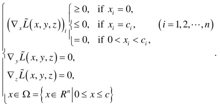
x yˆ ˆ, of the formula (4) is a unique optimal solution of the optimization question (4) and there exitssatisfies the following condition:
ˆ n
zR
0, if 0,
, , 0, if , 1, 2, ,
0, if 0 ,
.
, , 0,
, , 0,
0
i
x i i i
i i y
z
n
x
L x y z x c i n
x c
L x y z
L x y z
x x R x c
Equivalently, the point
x y zˆ ˆ ˆ, ,
satisfies the fol- lowing condition,
T
ˆ ˆ ˆ ˆ, , 0, ˆ ˆ ˆ, , 0,
ˆ ˆ ˆ, , 0.
x y
z
x x L x y z x
L x y z
L x y z
(5)
In order to discuss the constrained programming pro- blem (4), first, we define a augmented Lagrangian func- tion of (4) as follows
T 2T 2 T
2
2 T
, , ,
, ,
2
L x y z k f x y f x y
z f x pp y p
k
f x pp y p x
where is a penalty parameter and is an approximation of the Lagrange multiplier vector. Hence, the problem (4) can be solved by the stationary point of the following problem,
0
k z
, ,min , , ,
n
x y z R
L x y z k
(6)Then, the condition (5) can be written as
T
ˆ ˆ ˆ ˆ, , , 0, , ˆ ˆ ˆ, , , 0,
ˆ ˆ ˆ, , , 0.
x y z
x x L x y z k x
L x y z k
L x y z k
(7)
Now, we introduce the projection function P as
follows,
1
2
, , , ,
n
n
R P u P u P u P
where u , i
0, 0, , 0, , . ii i i
i i i
u
P u u u c
c u c
(8)
From the projection conclusion as shown in [19], the first inequality of (7) can be equivalently represented as
ˆ x ˆ ˆ, , ,ˆ
ˆ 0, 0. P x L x y z k x So the optimal solution of (4) and the stationary point of (6) meet with the conditions
2 T
, , , , 0,
, , , 0,
.
x
y
x
x P x L x y z k
L x y z k
f x pp y p
(9)
3. Stability Analysis of the Neural Network
Model
By Theorem 8 and Theorem 9 in [20], there exists a constant , such that if is an optimal solution of the problem (6), then
0
k c
x y z, ,
,
x y is an optimal solution of the problem (4) and
, ,
min , , , .
n
x y z R
L x y z k f x
Notice that L x y z
, ,
L x y z k
, , ,
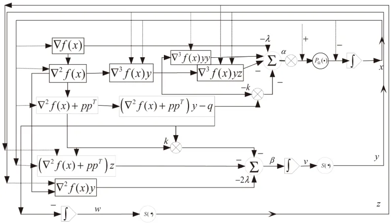
. By the Lagrange function defined above, we can describe the neural network model by the following nonlinear dynamic system for solving (10). The logical graph is shown in Figure 1.
3 33 2 T
2 2 T
2 T 2 T
2 T d , , d d , , d 2 d , , d
, 1, 2, , , 1, 2, ,
j j
k k
x
P x xL x y z x t
P x f x f x yy f x yz
k f x y f x pp y p x
v
yL x y z t
f x y f x pp z
k f x pp f x pp y p
w
zL x y z f x pp y p t
y s v j n
z s w k n
[image:3.595.63.282.220.324.2]Figure 1. Logical graph of the proposed neural network model.
0
,
T1 , 2 , , n , 0,
f x f x f x f x
T3 2 2 2
1 , 2 , , n
f x y f x y f x y f x y
d
, , , d
x
x P x xL x y z t
we have
0 0
d
e d e ,
and the activation function s
is continuouslydifferentiable and satisfies that s 0. It is easy to see that if c
x y, ,z
, then it is a equis an optimal solution of the problem (6) ilibrium point of network (10). Conversely, if
x y z, ,
is a equilibrium point of network (10), it m point of original problem (4). To analyze the convergence of the neural network (10), the following lemmas are first introduced (see [19]).Lemma 4 Assume n
ust be KKT
that the set is a closed
co aliti
R
nvex set, then the following two inequ es hold,
T
0, n, P x y xP x x R y
, , n
P x P y xy x y R
where P:Rn is a projection operator defined as
minP
For any in al poi
.
Lemma 5 iti nt
30 , 0 , 0
n
x t v t w t
R , there exists a unique continuous solution
x t
, ,
3nt of (1
v t w t R for (10). Moreover, x t
pro . The equilibrium poin 0) solves (5).Proof: By Assumption A1, P
vided that x t
0
x xL x y z k, , ,
x , yL x y z k
, , ,
and
2 T
f x pp y p
are lo According to local
cally Lipschitz continuous. existence theorem of ordinary differential equation, there exists a unique continuous solution
x t
,v t ,w t
of (10) for
t T0,
.Next, let initial point x t
0 . Since, d
d
t s t s
t t
x
x s P x xL x z s
t
ently,
.
y
Or equival
0
0
0
e t t e t tes , ,
t d
x t x t
P x xL x y z s So, x t
0 provided that x t
0 0,
, , ,
0P x xL x y z k
t t s
, and since
0 0
0
0
0
e e e , ,
e e e
e
t t t t
t t
t t
0 0
0
e t
t
d
x t x t P x xL x y z
x t
c c x t
c
s.
Thus,
c
x t re establishin
provided that
Befo g the converge m, we need the property of the following augmented Lagrangian fu
0x t . nce theore
nction.
Assumption 4 L x y z
, ,
satisfies the local mono- tone property of following definition about x .
T
, ,
x
L x y z L x y z
, , 0.
x
x
x
Now we are ready to establish the stability and the convergence results of network (10).
Theorem 6 Assume that f x
:RnR is strictly convex and the fourth differentiable, and
, ,
with x t
0 is chosen in a small neighborhood ofpoint, then the proposed neural network of (10) is stable in the sense of Lyap
conve he stationary point
, ,
the equ
unov and globally ilibrium
rgent to t x y z , where x is the optimal solution of (2).
Proof. We define V : R as follows:
2, 2
z f x
show that is a suitable Lyp ov c mic system (10), it is evident that
, ,
V x t y t z t
1
, ,
L x t y t t x t x
W fun
e want to tion for dyna
V un
1
2, , ,
2
V x t y t z t x t x
,
x t ,y t ,z t
x y z, ,
, ,
0.V x y z Then
1 1 T T d dd d d
, ,
d d d d d
d d d d d
, , .
n
i i i
i i i
x n
i i i i i
i i i i i i
x
x y
V L L L
u t y t z t
x x P x L x y z x dz d
dt i
And denote that
1 , 2 , ,
v n
Gdiag s v s v s v ,
1 , 2 , ,
w n
G diag s w s w s w
we have
x y v z w
L L L
x t y v t z w t
x x P x L x y z x
(11)
1 T T T T T T T d d dd d d
, , d d , , , , d d d , , d , , , , , , n i i i i
i i i i
x
x y v
z w x x x d d i
x v w
V L L L
s v s w
t x t y t z t
x x P x L x y z x
x v
L x y z L x y z G
t t
w L x y z G
t
x x P x L x y z x
L x y z P x L x y z x
x x
T T , , , , , , , , , , . xy v y
z w z
P x L x y z x
L x y z G L x y z
L x y z G L x y z
(12) In the first inequality of Lemma 4, let
, ,
x
x x L x y z and y x, then
C
T
, , , , , , 0.
x x x
P x L x y z x x L x y z P x L x y z
onsequently,
T T 2 T , , , , , , , , , , . x x x x xP x L x y z x L x y z
P x L x y z
x a x x L x y z
x x x P x L x y z
(13)
Then, we obtain from (12), (13) and Assumption A4
2
T T , , , , , , , , , , , , , , 0, xy v y
z w z
V
x y z P x L x y z x
x x L x y z
L x y z G L x y z
L x y z G L x y z
(14) T
dt x
d
d
, , 0
d V
x y z t
(15)
consequently, V P x t
,y t
,z t
by (14), it is evident this Lypunov
function, and at
d d d d
0 0, 0, 0.
t
d d d d
V x v w
t t t
By the Lypunov stability theory, systems (10) is le. Therefore, when t i
asymptotically stab he in tial point
x y x0, 0, 0
is obtain near to the equilibrium point, theset
x t
,y t ,z t
tt0
is bounded. By also using nvariant principle, the trajectory of the neural LaSall's inetwork (10)
u t
,y t ,z t
will converge to the ximum invariant subset of the following set
ma
d
, , 0 .
d V E x y z S
t
Assume again that
, ,
X x x y z E , then we have
lim , 0.
tdist x t X
X x , we have Specially, when
.t
limx t x
The proof is completed.
4. Numerical Examples
In order to verify the effectiveness of the presented algorithm in this paper, three examples were selected fr ese Examples has been used e new algorithms (see [1- om the literature [21]. Th
to check the effectiveness of th 5]).
For the first example, it is easy to verify that the Hessian matrix of the object function
1
22
p
f x F x
is rank one deficiency at the minimizer x. For the last two examples, the corresponding matrix is no
e procedure as n transformation as Hessian
nsingular at the minimizer. In order to adapt them to the singular case, we have adopt the sam
proposed in [1] by introducing functio follows,
T 1 T
:F x F x F x A A A A xx (16) where x is the root of F x
0 and
n m n1 T
F x :R R ,AR,A 1,1,,1 . Now we can construct the relevant objection function
p
f x
1
22
p
f x F x
fo an if
r which its Hessian matrix being rank one deficiency d the Interval
l h, includes the root of the original
F x
, it can be checked that the root of the originalF x min p
is the minimizer of the optimization problem
,f x l x h .
Ex. 1: Modified Powell Singular Function: a) n4,m4
1 1 10 2 3
b) f x x x x
1 2
3 4
5 2
f x x x
23 2 2 2 3
f x x x x
1 2
24 10 1 4
f x x x
c) at the minimizer Ex. e Function:
a)
b) 2
0 f 2: Beal
0, 0, 0, 0 .
x
2, 3 n m
1 1 1 1
f x y x x
2
2 2 1 1 2
f x y x x
1
1 2
3
3 3
f x y x x
1 1.5; 2 2.25; 3 2.625
y y y
c) at the minimizer
Ex. fied Broyden Tri ion:
a)
0 f 3: Modi
3, 0.5 .
x
diagonal Funct
4, 4 n m
b) f1
x 3 2 x x1
12x21
2 3 2 2 2 1 2
f x x x x x32
3 3 2 3 3 2 2 4 2
f x x x x x
4 3 2 4 4 3
f x x x x c) f 0
Meanwhile, we com at the minimizer
pare the vior of the proposed model with the classical pr ection gradient system [11] as follows,
1,1, 1 .
x
dynamic beha 1,
oj
dt P x f
d, 0
p
x
x x
(17)
simulate the dynamics of the corresponding systems. The integral curves a
by using the ODE function ode15s for the numerical
ch
for which the Hessian matrix at the minimizer is generally assumed to be nonsingular.
We use Matlab 7.0 to
re obtained
integration. For the proposed system (10) (PR) and the classical projection gradient system (10) (PG), we have osen the same initial point to numerically solve the ODEs.
For Ex.1, we choose x0
01, 0.9,1.5238,10.9605 ,
1
for both PR and PG and let y0 and 0
z be some random values between 0 and 12. The other parameters PR are chosen as l0, h20,
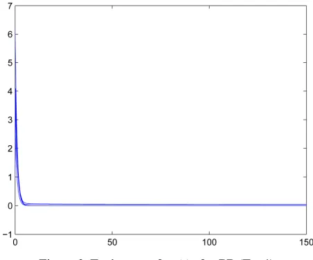
0.0000001,
k3000. The results are shown in Figures 2 and 3. It can b
urves response of PR converge to e seen, in Figure 2, that the
integral c fp ’s
nimizer
mi x
0, 0, 0, 0
. On the contrary, as shown in Figure 3, the curves of PG failed to converge to fp’sin
mini itial point.
For Ex. 2, we choose l 0,h 3, 0.0000001; mizer with the same
0 1, 6 ;
[image:6.595.309.535.539.727.2]x rand k5000, 1. Similar results are obtained, i.e., the proposed system PR successfully
found the minimizer while the classical system PG failed. Th shown in Figures 4 and 5 respectively.
Figures 6 and 7 show the corresponding results for Ex. 3 with initial conditions chosen as
3, 0.5
x
e results are
0 1, 1, 1, 1 ,
x 0, 1,
l h 0.0000001, k5000, 1, 100. got the minimizer PR got stuck all the The proposed
1,1,1,1
x time.
system PR , while the sy
finally stem
5. Concluding Remarks
Singular nonlinear convex optimization problems have been traditionally studied by classical numerical methods. In this paper, a novel neural network model was estab lished to solve such a difficult problem. Under some mil
assump ed n n
constraine
[image:7.595.305.539.84.698.2]mented Lagrange function, a neural - d tions, the unconstrain onlinear optimizatio problem is turned into a d optimization prob- lem. By establishing the relationship between KKT points and the aug
Figure 3. Trajectory of x t( ) for PG (Ex. 1).
Figure 4. Trajectory of x t( ) for PR (Ex. 2).
Figure 5. Trajectory of x t( ) for PG (Ex. 2).
Figure 6. Trajectory of x t( ) for PR (Ex. 3).
[image:7.595.59.286.330.733.2]REFERENCES
[1] R. B. Schnabel and T.-T. Chow, “Tensor Methods for Unconstrained Optimization Using Second Derivativ SIAM: SIAM Journal on Optimization, Vol. 1, No. 3, 1991, pp. 293-315. doi:10.1137/0801020
es,”
[2] D. Feng and R. B. Schnabel, “Tensor Methods for Equ lity Constrained Optimization,”SIAM: SIAM Journal on Optimization, Vol. 6, No. 3, 1996, pp. 653-673.
doi:10.1137/S1052623494270790
a-
[3] A. Bouaricha, “Tensor Methods for Large Sparse Uncon-strained Optimization,” SIAM: SIAM Journal on Optimi-zation, Vol. 7, No. 3, 1997, pp. 732-756.
doi:10.1137/S1052623494267723
[4] R. Ge and Z. Xia, “Solving a Type of Modified BFGS Algorithm with Any Rank Defects and the Local Q-S perliner Convergence Properties,” Journal of Computa-
tio atics , 2006
pp. 193-208.
Advances and Applications , pp.
17-35.
u , - nal and Applied Mathem , Vol. 22, No. 1-2 [5] R. Ge and Z. Xia, “A Type of Modified BFGS Algorithm
with Rank Defects and Its Global Convergence in Convex Minimization,” Journal of Pure and Applied Mathematics:
, Vol. 3, No. 1, 2010
[6] Y. S. Xia and J. Wang, “On the Stability of Globally Pro- jected Dynamical Systems,” Journal of Optimization Theory and Applications, Vol. 106, No. 1, 2000, pp. 129- 150. doi:10.1023/A:1004611224835
[7] Y. S. Xia and J. Wang, “A New Neural Network for Solv- ing Linear Programming Problems and Its Applications,” IEEE Transactions on Neural Networks, Vol. 7, No. 2, 1996, pp. 525-529. doi:10.1109/72.485686
[8] Y. S. Xia, “A New Neural Network for Solving Linear and Quadratic Programming Problems,” IEEE Transac- tions on Neural Networks, Vol. 7, No. 6, 1996, pp. 1544- 1547. doi:10.1109/72.548188
[9] Y. S. Xia, J. Wang, “A General Methodology for De- signing Globally Convergent Optimization Neural Net- works,” IEEE Transactions on Neural Networks, Vol. 9, No. 6, 1998, pp. 1331-1343. doi:10.1109/72.728383
[10] Y. S. Xia, “A Recurrent Neural Network for Solving Lin- ear Projection Equations,” IEEE Transactions on Neural Networks Vol. 13, No. 3, 2000, pp. 337-350.
doi:10.1016/S0893-6080(00)00019-8
[11] Y. S. Xia, H. Leung and J. Wang, “A Projection Neural Network and Its Application to Constrained Optimi
58.
zation
Problems,” IEEE Transactions on Circuits and Systems I, Vol. 49, No. 4, 2002, pp. 447-4
doi:10.1109/81.995659
[12] Y. S. Xia and J. Wang, “A General Projection Neural Network for Solving Monotone Variational Inequality and Related Optimization Problems,” IEEE Transactions on Neural Networks, Vol. 15, No. 2, 2004, pp. 318-328.
doi:10.1109/TNN.2004.824252
[13] X. Gao, L. Z. Liao and W. Xue, “A Neural Ne Class of Convex Quadratic Minimax P
twork for a roblems with Con- straints,” IEEE Transactions on Neural Networks, Vol. 15, No. 3, 2004, pp. 622-628. doi:10.1109/TNN.2004.824405
[14] C. Y. Sun and C. B. Feng, “Neural Networks for Non- convex Nonlinear Programming Pro
Control Approach,” Lec
blems: A Switching ture Notes in Computer Science, Vol. 3496, 2005, pp. 694-699.
doi:10.1007/11427391_111
[15] Q. Tao, X. Liu and M. S. Xue, “A Dynamic Genetic Al- gorithm Based on Continuous Neural Networks for a Kind of Non-Convex Optimization Problems,” Applied Mathematics and Computation, Vol. 150, No. 3, 2004, pp. 811-820. doi:10.1016/S0096-3003(03)00309-6
[16] D. J. Bell and D. H. Jacobson, “Singular Optimal Control Problems,” Academic Press, New York, 1975.
[17] F. Lamnabhi-Lagarrigue and G. Stefani, “Singular Opti-mal Control Problem: On the Necessary Conditions of Optimality,” SIAM: SIAM Journal on Control and Opti- mization, Vol. 28, No. 4, 1990, pp. 823-840.
doi:10.1137/0328047
[18] L. Liu, R. Ge and P. Gao, “A Novel Neural Network for Solving Singular Nonlinear Convex Optimization Prob- lems,” Lecture Notes in Computer Science, Vol. 7063, 2011, pp. 554-561. doi:10.1007/978-3-642-24958-7_64
[19] D. Kinderlehrer and G. Stampacchia, “An Introduction to
w and K. E. Hillstrom, “Testing Variational Inequalities and Their Applications,” Aca- demic Press, New York, 1980.
[20] X. Du, Y. Yang and M. Li, “Further Studies on the Heste- nes-Powell augmented Lagrangian Function for Equality Constraints in Nonlinear Programming Problems,” OR Transactions, Vol. 10, No. 1, 2006, pp. 38-46.
[21] J. J. More, B. S. Garbo