http://www.scirp.org/journal/tel ISSN Online: 2162-2086 ISSN Print: 2162-2078
DOI: 10.4236/tel.2016.65101 September 23, 2016
Commodity Arbitrage and the Law of One Price:
Setting the Record Straight
John Pippenger
Department of Economics, University of California, Santa Barbara, CA, USA
Abstract
A general consensus rejects effective commodity arbitrage and the law of one price. But this consensus is mistaken because it is based on research using retail prices where price differentials do not represent risk-free profits. Using commodity auction prices, a few articles support effective arbitrage and the LOP. Using longer intervals and a wider variety of commodities than ever before, this paper provides even stronger support for effective commodity arbitrage and the Law of One Price. In addition, for the first time, it uses commodity auction prices rather than retail prices to look for border effects and rejects them.
Keywords
Exchange Rates, Arbitrage, Law of One Price, Borders, Half Lives, Auction Markets
1. Introduction
Arbitrage and the Law of One Price (LOP) are basic implications of price theory. The failure to respond to risk-free profit opportunities would reject basic assumptions like profit and wealth maximization. But claims about arbitrage and the LOP are mixed. At least part of this confusion is the result of some authors using their own definitions for “arbitrage” and the “Law of One Price”. Imagine the confusion in physics if some re-searchers used their own special definitions for technical terms like “neutron” or “muon”!
There is a strong consensus that arbitrage is effective in financial markets and, as a
result, that the LOP holds in financial markets. For example [1] says that: “Evidence in
financial markets of an opportunity for pure arbitrage, and therefore a violation of the
law of one price, is considered an anomaly…”. While [2] says the following:
How to cite this paper: Pippenger, J. (2016) Commodity Arbitrage and the Law of One Price: Setting the Record Straight. Theoreti- cal Economics Letters, 6, 1017-1033.
http://dx.doi.org/10.4236/tel.2016.65101 Received: August 20, 2016
Accepted: September 20, 2016 Published: September 23, 2016 Copyright © 2016 by author and Scientific Research Publishing Inc. This work is licensed under the Creative Commons Attribution International License (CC BY 4.0).
1018
Arbitrage is one of the fundamental pillars of financial economics. It seems gener-ally accepted that financial markets do not offer risk-free arbitrage opportunities, at least when allowance is made for transaction costs.
This literature uses “arbitrage” and the “Law of One Price” as they are defined in dic-tionaries and encyclopedias.
On the other hand, the consensus is that arbitrage and the LOP fail in commodity markets. But this consensus is based on research that does not use the terms “arbitrage”
and the “Law of One Price” as they are defined in dictionaries and encyclopedias. [3]
describes that consensus as follows:
The Law of One Price states that international relative price differentials should be arbitraged away so that identical goods in different countries should sell for the same price when expressed in a common currency. Yet the evidence from the em-pirical literature shows that not only are relative prices quite different across countries, but also such deviations are highly volatile and persistent.
But the evidence that [3] refers to uses retail markets where price differentials do not
represent risk-free profits as is required by the definition of arbitrage and the Law of One Price found in the relevant dictionaries and encyclopedias.
References [4] [5] and the related research in commodity markets that supports
ef-fective arbitrage and the LOP uses auction markets where contracts can eliminate price uncertainty and price differentials can represent risk-free profits.
2. Literature Review
Subsection 2.1 reviews how dictionaries and encyclopedias devoted to economics define “arbitrage” and the “Law of One Price”. Subsection 2.2 reviews the research that uses retail prices to test the LOP. Section 2.3 reviews the literature on Border Effects, which also uses retail prices. Section 2.4 reviews the literature using commodity auction pric-es.
2.1. Definitions
Dictionaries and encyclopedias specializing in economics clearly define arbitrage as a
“risk-free” transaction1. For example, The New Palgrave Dictionary of Economics
be-gins the discussion of arbitrage as follows: “An arbitrage opportunity is an investment strategy that guarantees a positive payoff in some contingency with no possibility of a
negative payoff….”. Wikipedia (25 May 2010) says the following: “When used by
aca-demics, an arbitrage is a transaction that involves no negative cash flow at any proba-bilistic or temporal state and a positive cash flow in at least one state; in simple terms, it is a risk-free profit”.
These definitions imply that, for a commodity price differential to reject effective
ar-bitrage, it must represent a risk-free profit.
The following quote from The Penguin Dictionary of Economics is a fairly typical
1In this context “risk-free” refers to certainty regarding prices. As in all transactions, there is always the risk in
1019
definition of the Law of One Price:
The law, articulated by Jevons, stating that “In the same open market, at any mo-ment, there cannot be two prices for the same kind of article.” The reason is that, if they did exist, arbitrage should occur until the prices converge.
The New Palgrave Dictionary of Economics does not have a separate heading for the LOP. The law is discussed on page 189 under the heading of Arbitrage. “The assertion that two perfect substitutes (for example, two shares of stock in the same company) must trade at the same price is an implication of no arbitrage that goes under the name of the law of one price”.
These definitions of the Law of One Price imply that, for a price differential to reject
the LOP it must represent a risk-free profit.
The auction prices used in the financial literature and by [4] [5] and related research
using commodity auction prices are consistent with these definitions of arbitrage and the LOP because they can represent risk-free profits. That is not true of the research
re-ferred to by [3].
2.2. Retail Prices and the LOP
One cannot test the LOP as it is defined in dictionaries and encyclopedias in retail markets because retail price differentials do not represent risk-free profits. Suppose one grocery store sells seedless red grapes at $0.99 per pound and a store across the street sells them for $2.00 a pound. That price differential does not reject effective arbitrage and the LOP because one cannot buy them at $0.99 and sell them for $2.00 for a
risk-free profit2.
Several articles study international price convergence in retail markets and claim that they are testing the LOP. None find strong support for the LOP. Recent examples using
individual prices rather than indexes include [6]-[10]3.
The most influential is probably [6]. It uses prices for identical goods in duty free
stores on Scandinavian ferries. Reference [9] describes the results in [6] as follows: they
“find that the LOOP does not even hold for identical goods sold at the same location as long as these goods are denominated in different currencies…..”.
But arbitrage is not possible on those Scandinavian ferries or similar ferries around the world. No one on a Scandinavian ferry can buy a particular brand of vodka using Swedish kronor and then turn around and sell it back to the duty free store for Finnish
markka. As a result, the price differentials in [6] do not reject effective arbitrage and the
LOP because they do not represent risk-free profits.
The same problem applies to all supposed tests of the LOP using retail prices; those price differentials do not represent risk-free profits. Retail stores sell at retail prices.
2Arbitrage also is not possible in most wholesale markets. Brand names and marketing contracts usually
pre-vent arbitrage. For example there are no active forward markets for Kleenex. But there are exceptions like wholesale markets for fresh fish and flowers. It is possible to buy live lobsters at the wholesale market in Bos-ton on Monday and simultaneously sell them in London for delivery later that week. But that is not true for frozen lobster where there are brand names and no active wholesale markets.
1020
They do not buy at retail, they buy at wholesale. Put bluntly, at the retail level all goods
are “non-traded” because no one, not even duty free stores on Scandinavian ferries, both buys and sells at retail.
There is another problem with the use of retail prices. The exchange rates typically used to convert foreign retail prices into domestic equivalents are auction prices. For
example [6] uses end-of-month rates from the IMF’s International Financial Statistics.
Expectations drive auction prices like exchange rates. They do not drive retail prices. Mixing retail commodity prices and auction exchange rates in this way artificially increases the volatility of the converted commodity retail prices and reduces the corre-lation between domestic and foreign prices. Using auction commodity prices and auc-tion exchange rates eliminates this mixture of retail and aucauc-tion prices.
Although arbitrage is not possible at the retail level, there are economic links be-tween international retail commodity markets. One link works from the domestic retail market through the domestic wholesale market to the foreign wholesale market and then through that market to the foreign retail market.
Another link operates from the domestic retail market through domestic production
to domestic auction markets like those in Table 1 then through those markets to
for-eign auction markets, forfor-eign production and finally forfor-eign retail markets. These indi-rect links between international retail markets are not very strong in the short run, but they presumably provide the long-run link that we see in tests of the Law of One Price
and Purchasing Power Parity using retail price indexes4. However using auction prices
produces much stronger short-run links.
2.3. Border Effects
Several articles estimate Border Effects using retail indexes or prices. They include [12]-[18]5. They appeal to either arbitrage or the LOP, or both, and reject them6.
Reference [13] for example says the following:
In Figure 2, we repeat the exercise for 1990. The comparison with Figure 1 is striking. The between-country distribution has diverged from the two within country distributions. Japanese prices expressed in US dollars have risen even more relative to US prices. The violation of the law of one price became even more severe.
But the price differentials [13] refers to do not reject effective arbitrage and the Law
of One Price as they are defined in the relevant dictionaries and encyclopedias because their retail price differentials do not represent risk-free profits. In addition, in con-structing those differentials they use auction exchange rates, which are driven by ex-pectations, and retail prices, which are not driven by expectations.
Given the weak links between international retail markets discussed above, we should expect relatively wide borders at the retail level. But those wide borders do not reject
4See [11] for a fairly recent review of PPP. 5Dissenting articles include [19] and [20].
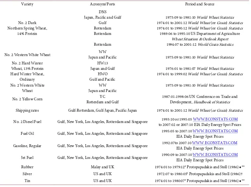
1021 Table 1. Products, intervals, and sources.
Variety Acronym/Ports Period and Source
No. 2 Dark Northern Spring Wheat,
14% Protein
DNS Japan, Pacific and Gulf
Gulf Rotterdam Rotterdam Rotterdam
1975:09 to 1981:10 World Wheat Statistics 1974:01 to 2001:12 World Wheat (or Grain) Statistics 1974:01 to 1990:12 World Wheat (or Grain) Statistics 1989:06 to 1995:10 US Department of Agriculture
Wheat Situation & Outlook Report 1994:07 to 2001:12 World Grain Statistics No. 2 Western White Wheat Japan and Pacific WW 1975:09 to 1981:10 World Wheat Statistics
No. 2 Hard Winter
Wheat, 13% Protein Japan and Gulf HW13 1976:01 to 1981:07 World Wheat Statistics Hard Winter Wheat,
Ordinary Gulf and Pacific HWO 1974:01 to 1999:02 World Wheat (or Grain) Statistics No. 2 Western White
Wheat Japan and Pacific WW 1975:09 to 1981:10 World Wheat Statistics No. 2 Yellow Corn Rotterdam and Gulf YC 1987:01-1998:06 UN Conference on Trade and Development, Handbook of Statistics
Shipping rates Gulf-Rotterdam, Gulf-Japan, Pacific-Japan 1974:01 to 2001:12 World Wheat (or Grain) Statistics No. 2 Diesel Fuel Gulf, New York, Los Angeles, Rotterdam and Singapore to 2007:02 or 2007:10 EIA Daily Energy Spot Prices 1993:10 or 1995:05 WWW.ECONSTATS.COM
Fuel Oil Gulf, New York, Los Angeles, Rotterdam and Singapore 1995:05 to 2007:10 EIA Daily Energy Spot Prices WWW.ECONSTATS.COM Gasoline, Regular Gulf, New York, Los Angeles, Rotterdam and Singapore 1992:07to 2007:10 EIA Daily Energy Spot Prices WWW.ECONSTATS.COM Jet Fuel Gulf, New York, Los Angeles, Rotterdam and Singapore 1990:09 to 2007:10 EIA Daily Energy Spot Prices WWW.ECONSTATS.COM Rubber Malay and UK 1974:01 to 1979:12a Protopapadakis and Stoll (1986)♦**
Silver US and UK 1972:07 to 1980:05a Protopapadakis and Stoll (1986)†
Tin US and UK 1974:01 to 1980:07a Protopapadakis and Stoll (1986)♦**
aWeekly. Original Sources: **Financial Times (UK). ♦Journal of Commerce (N.Y.). †Samuel Montague.
the LOP and effective arbitrage because the retail price differentials do not represent potential risk-free profits. However one can evaluate commodity arbitrage and the LOP in auction markets where risk-free profits are possible.
2.4. Auction Markets
Several articles use commodity prices and exchange rates from auction markets to
eva-luate commodity arbitrage and the LOP. See [4] [5] [11] [21]-[24]. With the exception
of [11] [21] they all use monthly grain prices7. This research is much more supportive
of effective arbitrage and the LOP.
3. New Evidence
To produce risk-free profits, commodity arbitrage normally requires three
“simultane-7Note that the monthly prices are usually averages of daily closing prices and that averaging introduces
1022
ous” transactions8: 1) buying a commodity spot or with a nearby futures contract in one
location, 2) arranging for the shipping of the commodity to a second location and 3) selling the commodity in that second location when it is due to arrive. The first and third transactions normally require active auction markets. The second requires active markets where arbitragers can find the necessary transportation as needed.
Forward contracts pose practical problems for testing commodity LOP because for-ward prices are difficult to find. I have neither the time nor the resources to do so. Like most previous work using commodity auction prices, I am forced to use spot prices.
Fortunately, as [26] and [27] show, while forward exchange rates are highly biased
es-timates of future spot exchange rates, forward commodity markets provide better esti-mates of future commodity prices. So while my price differentials also do not represent risk-free profits, they come much closer to doing so than research using retail prices.
3.1.
Grains
References [4] [5] [22] [24] use shorter versions of these grain prices and freight rates
to test the LOP. But only [24] estimates half Lives.
The top half of Table 1 describes the sources for grain prices. Between the US and
Rotterdam prices cover over 25 years. Earlier research covers only 10 to l1 years. Freight rates for wheat vary with the size of the ship and at times more than one rate is
published. These are the same as in [4]. Unlike prices, freight rates are not spot.
Foot-notes in World Wheat Statistics describe the freight rates as follows: “Estimated mid-
month rates based on current chartering practices for vessels to load six weeks ahead.” Freight rates are forward, not spot, prices. These forward rates imply that there is an active forward market for shipping grain.
These grain prices have several advantages: 1) “identical” products, 2) all prices in dollars, 3) freight rates are available for wheat, 4) for Rotterdam wheat prices cover an unusually large number of years, about 25, 5) export prices are free on board (FOB) and import prices include certificates, insurance and freight (CIF), (For Japan, prices do not include insurance.) and 6) most important of all, arbitrage should be possible in all these markets.
The first part of Table 1 describes the types of grains, data sources, ports and the
acronyms used later to identify the different grains. A “J”, “P”, “G” or “R” attached to an acronym indicates the port. For example, DNSR is Dark Northern Spring wheat at Rotterdam.
For trade with Japan, I use the same intervals used earlier by [4] [5] [24]. For a visual
inspection of that data, see [4]. I do not extend the Japanese data for two reasons: 1)
starting in 1982 several months of Japanese prices are missing and 2) in the 1990s Ja-pan erected non-tariff barriers to wheat imports that created artificial price differen-tials9.
8If the transaction is international, there will normally be a fourth contract to convert the foreign currency
obtained from the foreign sale back to the domestic currency.
1023
Wheat is a “heavy” grain. For wheat, one metric ton equals 36.7437 bushels. For corn, one metric ton equals 39.3682 bushels. Since a metric ton of corn takes up more space than a metric ton of wheat, I would expect freight rates for corn to be slightly higher than for wheat. Unfortunately I do not have separate freight rates for corn. I apply the freight rates for wheat to corn. Since the difference should be small and the two freight rates should move together, applying freight rates for wheat to corn should not be a se-rious problem.
Reference [22] also uses corn prices between the US and Rotterdam, but their data
cover only six years. The corn prices in Table 1 start as soon as they are available from
UNCTAD’s Handbook of Statistics and cover about 11 years. They end in mid 1998
because about then Europe began to impose restrictions on importing genetically mod-ified foods and most corn grown in the United States is genetically modmod-ified.
Some grain prices are missing. Except for DNSR during the early 1990s, there are never more than two missing months in a row. When only one month is missing, it is replaced with the previous month. When two months in a row are missing, the first month is replaced with the preceding month and the second month is replaced with the
following month10.
In the early 1990s, about 18 months of data are missing for DNSR and then a few
months later about another six months are missing. As Table 1 indicates, there is a
second source for the missing data, but where they overlap the two sources do not al-ways agree. It is possible to use the USDA data to fill in the missing data from World Grain Statistics, but the replacement produces unusual error terms that require long lags in tests for unit roots and cointegration. Those long lags reduce the significance of the tests. As an alternative, where there are USDA prices for DNSR, I report separate results using those prices for Rotterdam with freight rates and Gulf prices from World Grain Statistics.
3.2. Rubber, Metals and Petroleum
The latter half of Table 1 describes the additional prices, relevant ports, intervals and
sources. Rubber and metal prices are for Wednesdays and were supplied by [11] and
[21] who describe them in more detail.
Rubber prices may not be for identical products. For each Wednesday, the Journal of
Commerce quotes a single price for rubber in London. In another section it quotes US prices for several different grades that on a given day can range in price from 26.25 to 42.75 cents per pound. As a result, there is a strong possibility that the rubber prices are not for identical products.
All petroleum prices, both at US and foreign ports, are monthly averages of closing daily prices in dollars. Foreign prices are converted into US dollars using the closing dollar price of the foreign currency for that day. To the best of my knowledge, this is the first time that a wide range of petroleum prices have been used to test the LOP.
1024
3.3. Test Equations
There are freight rates for wheat. The direction of trade for grains is known because the United States is a major exporter and US prices are FOB while foreign prices are CIF. For grains one can account for the relevant shipping costs by computing the price dif-ferentials as the foreign forward CIF price minus the spot US FOB price plus the freight
rate. That approach produces a test equation where ut should represent insurance,
cer-tificates and bid-ask spreads.
( ) (
1)
ln Pt+F −ln ptD+ ft =ut (1)
( )
1ln Pt+F is the log of the dollar price of grain at time t in a foreign port one month
forward. ln
(
ptD+ ft)
is the log of the spot price in the appropriate US port plus thefreight rate for loading at time t. After accounting for other costs, ln
( ) (
1 ln)
F D
t t t
P+ − p + f
should represent potential risk-free profits.
Two critical parts of that test equation are missing: ft, the freight rate for loading at
time t, and 1
F t
P+, the forward price for t + 1. But ft−1 can serve as a proxy for ft because
ft−1 is the price for loading in a bit less than two weeks.
Fortunately forward commodity prices appear to be reasonable estimates of future
spot commodity prices. As a result, the future spot price 1
F t
p+ can serve as a proxy for
1
F t
P+.
Replacing ft with ft-1and 1
F t
P+ with ptF+1 provides a measure of price differentials for
grains.
( ) (
1 1)
ln F ln D
t t t t t
p+ − p + f− =u +ε (2)
where εt is the additional error due to using ft−1 as a proxy for ft and 1
F t
p+ as a proxy for
1
F t
P+.
The lack of information about freight rates and the direction of trade for the other products requires a different measure of price differentials for those products.
( ) ( )
ln ptF −ln ptD =zt (3)
Equation (3) is the price differential normally used in the commodity LOP and Bor-ders literature.
Using Equation (3) with grain prices provides consistent tests for all products and also provides some insight regarding the importance of time and transportation costs.
Like most auction prices, these have unit roots. Reference [24] shows that ln
( )
1F t
p+
and ln
(
1)
D t t
p + f− are cointegrated and that the corresponding differentials are
sta-tionary. To save space I do not replicate their results or report similar results for
( )
ln F t
p and ln
( )
D tp .
Reference [29] shows that ln
( )
ptF and ln( )
ptD are cointegrated and that( ) ( )
ln ptF −ln ptD are stationary, which implies that the price differentials in Equations
(2) and (3) are stationary. Given that stationarity, the next step is to estimate half lives for all pairs of commodities.
3.4. Half Lives
1025
1 1
N
t t i t i
i
X α βX− γ X−
=
= + +
∑
∆ (4)Xt is the price differential using either Equation (2) or (3). When Xt is AR (1), half
lives are calculated using Ln(0.5)/Ln(β). When Xt is AR(2) or longer, half lives are
cal-culated using impulse responses as [31] suggest.
Estimates of Equation (4) use both Equations (2) and (3) for grain prices and just Equation (3) for all other prices. Estimates use a variety of error tests: LM, Arch and two Q tests. There is also a Jarque-Bera test for normality. The only test that is signifi-cant is the one for normality. As expected, residuals have fat tails.
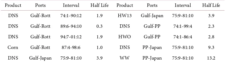
To save space, I omit the estimates of Equation (4). They are in [29]. Tables 2-4
re-port the half lives implied by those estimates.
Table 2 reports the half lives for grains implied by ln
( ) ( )
ptF −ln ptD . The average half life is four months.Table 3 reports the half lives for grains implied by ln
( ) (
1 ln 1)
F D
t t t
p+ − p + f− . While
the average half life in Table 2 is four months, in Table 3 it is only 1.1 months.
Omit-ting transportation costs and ignoring time substantially increases half lives for grains and, one would presume, does the same for other half lives.
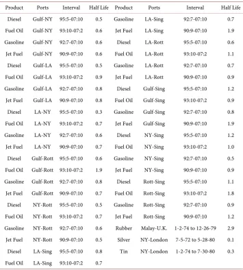
Table 4 reports the half lives for petroleum products, rubber and metals using
( ) ( )
ln ptF −ln ptD . The average half life in Table 4 is 1.1 months11.
As [6] points out, when using retail prices, half lives for price differentials commonly
run between 3 to 5 years. Although they have the best retail data, [6] cannot reject at
[image:9.595.194.555.451.552.2]even the 10% level that their differentials have unit roots, which would imply that their half lives are infinite.
Table 2. Half lives for grains measured in months using Equation (3).
[image:9.595.194.555.585.688.2]Product Ports Interval Half Life Product Ports Interval Half Life DNS Gulf-Rott 74:1-90:12 1.9 HW13 Gulf-Japan 75:9-81:10 3.9 DNS Gulf-Rott 89:6-94:10 0.3 DNS Gulf-PP 74:1-99:4 2.3 DNS Gulf-Rott 94:7-01:12 1.9 HWO Gulf-PP 74:1-86:4 2.8 Corn Gulf-Rott 87:4-98:6 1.0 DNS PP-Japan 75:9-81:10 9.3 DNS Gulf-Japan 75:9-81:10 3.9 WW PP-Japan 75:9-81:10 13.2
Table 3. Half lives for grains measured in months using Equation (2).
Product Ports Interval Half Life Product Ports Interval Half Life DNS Gulf-Rott 74:1-90:12 1.0 HW13 Gulf-Japan 75:9-81:10 0.7 DNS Gulf-Rott 89:6-94:10 1.5 DNS Gulf-PP 74:1-99:4 1.3 DNS Gulf-Rott 94:7-01:12 1.2 HWO Gulf-PP 74:1-86:4 1.1 Corn Gulf-Rott 87:4-98:6 0.9 DNS PP-Japan 75:9-81:10 0.9 DNS Gulf-Japan 75:9-81:10 1.8 WW PP-Japan 75:9-81:10 1.0
1026
Table 4. Half lives measured in months for petroleum products, rubber and metals.
Product Ports Interval Half Life Product Ports Interval Half Life Diesel Gulf-NY 95:5-07:10 0.5 Gasoline LA-Sing 92:7-07:10 0.7 Fuel Oil Gulf-NY 93:10-07:2 0.6 Jet Fuel LA-Sing 90:9-07:10 1.9 Gasoline Gulf-NY 92:7-07:10 0.6 Diesel LA-Rott 95:5-07:10 0.6 Jet Fuel Gulf-NY 90:9-07:10 0.6 Fuel Oil LA-Rott 93:10-07:2 1.1 Diesel Gulf-LA 95:5-07:10 0.5 Gasoline LA-Rott 92:7-07:10 0.7 Fuel Oil Gulf-LA 93:10-07:2 0.9 Jet Fuel LA-Rott 90:9-07:10 0.9 Gasoline Gulf-LA 92:7-07:10 0.8 Diesel Gulf-Sing 95:5-07:10 1.2 Jet Fuel Gulf-LA 90:9-07:10 0.8 Fuel Oil Gulf-Sing 93:10-07:2 0.9 Diesel LA-NY 95:5-07:10 0.3 Gasoline Gulf-Sing 92:7-07:10 0.8 Fuel Oil LA-NY 93:10-07:2 0.7 Jet Fuel Gulf-Sing 90:9-07:10 1.9 Gasoline LA-NY 92:7-07:10 0.6 Diesel NY-Sing 95:5-07:10 1.2 Jet Fuel LA-NY 90:9-07:10 0.7 Fuel Oil NY-Sing 93:10-07:2 1.0 Diesel Gulf-Rott 95:5-07:10 0.6 Gasoline NY-Sing 92:7-07:10 0.5 Fuel Oil Gulf-Rott 93:10-07:2 1.9 Jet Fuel NY-Sing 90:9-07:10 0.9 Gasoline Gulf-Rott 92:7-07:10 0.8 Diesel Rott-Sing 95:5-07:10 1.1 Jet Fuel Gulf-Rott 90:9-07:10 0.7 Fuel Oil Rott-Sing 93:10-07:2 1.8 Diesel NY-Rott 95:5-07:10 0.5 Gasoline Rott-Sing 92:7-07:10 0.9 Fuel Oil NY-Rott 93:10-07:2 0.7 Jet Fuel Rott-Sing 90:9-07:10 1.2 Gasoline NY-Rott 92:7-07:10 0.6 Rubber Malay-U.K. 1-2-74 to 12-26-79 2.9 Jet Fuel NY-Rott 90:9-07:10 0.5 Silver NY-London 7-5-72 to 5-28-80 0.1 Diesel LA-Sing 95:5-07:10 0.8 Tin NY-London 1-2-74 to 7-30-80 0.3 Fuel Oil LA-Sing 93:10-07:2 0.7
On the other hand, the half lives in Tables 2-4 are measured in months, not years.
Many of them are measured in fractions of a month. I conjecture that with better data they would be measured in weeks, days or even fractions of a day like the deviations from CIP.
Half lives in Tables 2-4 do not show any obvious signs of border effects. Half lives
between international ports like New York and Rotterdam are not obviously larger than between New York and Los Angeles. The next section, for the first time, uses auction prices to evaluate “Border Effects”.
3.5. Border Effects
Although the Borders literature uses other explanatory variables, it concentrates on how distance and borders affect the variance or standard deviation of changes in logs of
ratios of prices like F D
t t
p p . The log of F D
t t
p p is usually denoted Pt with the first
1027
it is often impossible to reject an infinite half life for retail price differentials even when the products are identical.
Standard deviations of ∆Pt and half lives of Pt are both natural measures of market
integration, but they measure different things. Consider the spectrum for ∆Pt. The area
under the spectrum for ∆Pt is the variance. The half life for Pt reflects how quickly that
spectrum falls as frequency falls. As a result, half lives for Pt and variances for ∆Pt can
be very different.
An extreme case would be where variances in ∆Pt are small and spectra flat. Small
standard deviations reject segmentation. Flat spectra imply infinite half lives. Or
va-riances for ∆Pt could be very large and spectra fall rapidly as frequency goes to zero.
Now standard deviations would support segmentation and half lives reject segmenta-tion. The bottom line is that neither half lives nor standard deviations are ideal meas-ures of integration. Here the two measmeas-ures agree; both standard deviations and half lives imply that international commodity auction markets are highly integrated.
Although there are many auction markets for commodities, there are far fewer auc-tion markets than retail markets. As a result, the number of commodities evaluated here is far smaller than in most of the Borders literature. To avoid unnecessary reduc-tions in degrees of freedom, tests use just borders and distance to evaluate Border
Ef-fects12. When there is a border, the border dummy is one. Otherwise it is zero. Distance
is the logarithm of the distance measure. There are three measures of distance: 1) dis-tance by ship (Ship), 2) disdis-tance as the crow flies (Crow), and 3) disdis-tance by highway
(Highway)13. For Ship, distance is measured as the shortest distance by sea. The source
for Ship is PORTWORLD.COM. For Highway it is MAPQUEST.COM. For Crow it is GeoBYTES.com/CityDistanceTool.htm.
Between portslike New York and Rotterdam, Ship is clearly the appropriate way to measure distance. Highways do not exist, and both great circle routes and “as the crow flies” can seriously understate the actual distance traveled. As a result, I use only Ship between international ports. I use all three measures between ports in the United States because it is not clear which is appropriate. To move products by ship from Los An-geles to New York by the shortest route they must go through the Panama Canal. The alternative is to ship by train or truck, which is much shorter but more expensive per mile.
It seems unlikely that grains or petroleum products would be shipped between New York and Los Angeles. If grain prices are higher in New York than Los Angeles, grain shipments from the Midwest would be diverted from Los Angeles to New York rather than shipped to Los Angeles by train or truck and then sent to New York by ship.
Something similar applies to petroleum products. Oil refineries are scattered around the United States with production and refineries concentrated in Louisiana, Oklahoma and Texas. As a result, conventional arbitrage probably does not operate between New York and Los Angeles. If petroleum prices are relatively high in New York, shipments
12Using dummies for classes of products such as grains, metals and oil produces similar results.
13Pacific ports are measured from Seattle, Gulf ports from New Orleans, Japan from Tokyo, Malay from Johor
1028
from Oklahoma or Louisiana are diverted from Los Angels to New York rather than sent to Los Angeles and then shipped to New York. This difference in market structure between international and domestic ports may help explain the “negative” Border Ef-fects reported below where borders appear to increase integration.
3.5.1. Borders and Half Lives
I use Equation (5) to evaluate Border Effects using half lives.
j j j
Z = +a dD +bB (5)
Zj is the log of a half life, e.g., for Diesel between NY and Rotterdam. Dj is the log of
distance, e.g., the log of Ship between the two ports. Bj is a border dummy that is one
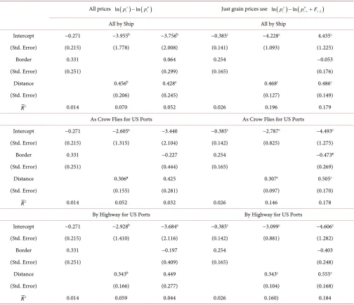
when there is a border and zero otherwise14. Table 5 reports the estimates of Equation
(5) using half lives.
On the left-hand side of Table 5, all half lives are for logs of F D
t t
p p . On the right-
hand side, half lives for just grains are for logs of 1
(
1)
F D
t t t
p+ p + f− while all other half
lives are for logs of F D
t t
p p . The first column on both sides excludes distance. The
second excludes the border. The third includes both.
In the first third of Table 5 all distance is by Ship. In the next third distance between
just US ports is by Crow. In the last third distance between just US ports is by Highway. Although cumbersome, this arraignment should reveal how different measures of dis-tance affect the results.
There is no evidence in Table 5 of a border effect in the sense that borders inhibit
trade. Estimates of b are never positive and significant. When Dj is included, b is usually
negative. How distance is measured does not appear to be important. The results for
distance are similar in all three parts of Table 5.
Distance itself is important. In the left-hand side, when B is excluded, d is always
sig-nificant. When B is included, most of the significance disappears. That result suggests
some multicolinearity. That multicolinearity largely disappears in the right-hand side.
Whether or not B is included, in the right-hand side d is always significant at the 1
per-cent level15.
When using half lives and spot auction prices, there is some suggestion that borders might increase integration. Standard deviations produce even stronger evidence of such an effect.
3.5.2. Borders and Standard Deviations
Presumably the Borders literature uses variances or standard deviations rather than half
lives because it is difficult to reject a unit root for retail Pt. As pointed out earlier,
auc-tion Pt are stationary.
To save space, I do not report the standard deviations. The relevant tables are in [29].
But some of their characteristics are interesting.
14Later Z
j is the log of the standard deviation of ∆Pt. Using actual half lives and standard deviations rather
than their logs produces similar, but somewhat weaker, results.
15Excluding tin, silver and rubber where there is at most one US port produces similar, but slightly weaker,
1029 Table 5. Estimates of Equation (5) using half lives.
All prices ln
( )
J ln( )
Pt t
p − p Just grain prices use ln
( )
ln(
1 2)
J P
t t t
p − p− +F−
All by Ship All by Ship
Intercept −0.271 −3.955b −3.756b −0.385c −4.228c 4.435c
(Std. Error) (0.215) (1.778) (2.008) (0.141) (1.093) (1.225) Border 0.331 0.064 0.254 −0.053 (Std. Error) (0.251) (0.299) (0.165) (0.176) Distance 0.456b 0.428a 0.468c 0.486c
(Std. Error) (0.206) (0.245) (0.127) (0.149)
2
R 0.014 0.070 0.052 0.026 0.196 0.179
As Crow Flies for US Ports As Crow Flies for US Ports
Intercept −0.271 −2.605a −3.440 −0.385c −2.787c −4.493c
(Std. Error) (0.215) (1.315) (2.104) (0.142) (0.825) (1.275) Border 0.331 −0.227 0.254 −0.473a
(Std. Error) (0.251) (0.444) (0.165) (0.269) Distance 0.306a 0.425 0.307c 0.505c
(Std. Error) (0.155) (0.281) (0.097) (0.170)
2
R 0.014 0.052 0.032 0.026 0.146 0.178
By Highway for US Ports By Highway for US Ports
Intercept −0.271 −2.928b −3.684a −0.385c −3.099c −4.606c
(Std. Error) (0.215) (1.410) (2.116) (0.142) (0.881) (1.282) Border 0.331 −0.197 0.254 −0.403 (Std. Error) (0.251) (0.409) (0.165) (0.248) Distance 0.343b 0.449 0.343c 0.555c
(Std. Error) (0.166) (0.277) (0.104) (0.168)
2
R 0.014 0.059 0.044 0.026 0.160) 0.184
aSignificant at 10% level. bSignificant at 5% level. cSignificant at 1% level.
These standard deviations are much smaller than the ones for retail prices. For
ex-ample, the average variance for ∆Pt in Table 2 of [32] is 2.12. The implied standard
deviation of 1.46 is almost 10 times larger than the largest of the standard deviations
using auction prices. The large standard deviations using commodity retail prices are at least partly the result of mixing sticky retail prices and volatile auction exchange rates. Using auction commodity prices solves this problem.
Including freight rates and lagging export prices generally reduces half lives for
grains, but generally increases standard deviations16. The average for grains using
16This difference is probably due at least partly to ε
t. The use of proxies tends to increase the short-run
1030
( ) ( )
ln ptJ −ln ptP , is 0.03. The average using ptF+1
(
ptD+ ft−1)
is 0.05. This differenceillustrates the point made earlier that half lives and standard deviations measure differ-ent things. Although they measure differdiffer-ent things, here they produce similar results. Both reject wide borders for commodity auction markets.
Table 6 is identical to Table 5 except that in Table 6 the Zj are standard deviations
rather than half lives. When Bj appears alone in Table 6, b is always negative, but never
significant. When Dj appears alone, d is always positive, but significant only when by
ship. When Dj and Bj appear together, d is positive and usually significant. But b is
al-ways negative and significant in Table 6.
With half lives in Table 5, b is occasionally negative, but never negative and
signifi-cant. In Table 6, all b are negative and some are significant at the 1% level. Excluding
[image:14.595.48.551.292.693.2]tin, silver and rubber produces similar, but slightly weaker, results.
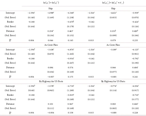
Table 6. Estimates of Equation (5) using standard deviations.
( )
( )
ln J ln P
t t
p − p ln
( )
1 ln(
1)
J P
t t t
p+ − p +F−
Ship Ship
Intercept −2.594c −4.909c −6.368c −2.516c −4.621c −5.939c
(Std. Error) (0.140) (1.169) (1.238) (0.104) (0.853) (0.870) Border −0.180 −0.470b −0.162 −0.424c
(Std. Error) (0.164) (0.179) (0.121) (0.126) Distance 0.254a 0.463c 0.231b 0.420b
(Std. Error) (0.136) (0.151) (0.099) (0.106)
2
R 0.004 0.046 0.145 0.015 0.079 0.235
As Crow Flies As Crow Flies
Intercept −2.594b −3.436c −6.876c −2.516c −3.189c −6.125c
(Std. Error) (0.140) (0.879) (1.265) (0.104) (0.901) Border −0.180 −0.934c −0.162 −0.792c
(Std. Error) (0.164) (0.267) (0.121) (0.190) Distance 0.084 0.574 0.066 0.484c
(Std. Error) (0.104) (0.169) (0.077) (0.120)
2
R 0.004 −0.007 0.175 0.015 −0.005 0.241
By Highway for US Ports By Highway for US Ports
Intercept −2.594b −3.578c −6.718c −2.516c −0.774c −6.056c
(Std. Error) (0140) (0.945) (1.289) (0.104) (0.114) (0.917) Border −0.180 −0.819c −0.162 −0.710c
(Std. Error) (0.164) (0.249) (0.121) (0.177) Distance 0.101 0.543c 0.083 0.466c
(Std. Error) (0.111) (0.169) (0.083) (0.120)
2
R 0.004 −0.004 0.158 0.015 −0.000 0.228
1031
Using Ship, Crow or Highway makes little difference. Using squares, square roots or reciprocals produces similar results. For auction prices, Border Effects appear to be
negative. Standard deviations for ∆Pt are generally smaller when there is a border.
Why?
The market structure in the US is the most likely explanation for the negative Border Effect. Shipping products from where they are produced to where the price is higher is more cost effective than conventional arbitrage between New York and Los Angeles. If prices are higher in New York than in Los Angeles, goods are not shipped from LA to NY. Instead grain or petroleum products that would have been shipped to LA are shipped to NY instead.
4. Summary
Dictionaries and encyclopedias clearly define arbitrage as a “risk-free” transaction. They also make it clear that the Law of One Price depends on effective arbitrage. As a result, for commodity price differentials to reject effective arbitrage and the Law of One price, they must represent risk-free profits.
Using retail prices, the Borders literature and most of the commodity LOP literature claim that arbitrage is ineffective and that the LOP fails. This view of commodity arbi-trage and the LOP seems to be the conventional wisdom. Pointing out that that con-ventional wisdom is mistaken because the retail price differentials used in that literature do not represent risk-free profits is a major objective of this article.
Using auction prices where arbitrage is possible, both the finance literature and the commodity literature support effective arbitrage and the Law of One Price. Using a wider range of commodity auction prices over longer intervals than before, my results reinforce that support for effective commodity arbitrage and the Law of One Price and also reject Border Effects.
References
[1] Armitrage, S., Chakarvarty, S.P., Hodgkinson, L. and Wells, J. (2012) Are There Arbitrage Gaps in the UK Gilt Strips Market? Journal of Banking and Finance, 36, 3080-3090.
http://dx.doi.org/10.1016/j.jbankfin.2012.07.001
[2] Akram, Q.F., Rime, D. and Sarno, L. (2008) Arbitrage in the Foreign Exchange Market: Turning on the Microscope. Journal of International Economics, 76, 237-253.
http://dx.doi.org/10.1016/j.jinteco.2008.07.004
[3] Lee, I. (2008) Goods Market Arbitrage and Real Exchange Rate Volatility. Journal of
Ma-croeconomics, 30, 1029-1042. http://dx.doi.org/10.1016/j.jmacro.2007.06.001
[4] Michael, P., Nobay, A.R. and Peel, D. (1994) Purchasing Power Parity yet Again: Evidence from Spatially Separated Commodity Markets. Journal of International Money and
Finance, 13, 637-657. http://dx.doi.org/10.1016/0261-5606(94)90036-1
[5] Pippenger, J. and Phillips, L. (2008) Some Pitfalls in Testing the Law of One Price in Com-modity Markets. Journal of International Money and Finance, 27, 915-925.
http://dx.doi.org/10.1016/j.jimonfin.2008.05.003
1032
[7] Haskel, J. and Wolf, H. (2001) The Law of One Price—A Case Study. Scandinavian Journal
of Economics, 103, 545-558. http://dx.doi.org/10.1111/1467-9442.00259
[8] Lutz, M. (2004) Pricing in Segmented Markets, Arbitrage Barriers, and the Law of One Price: Evidence from the European Car Market. Review of International Economics, 12, 456-475. http://dx.doi.org/10.1111/j.1467-9396.2004.00461.x
[9] Goldberg, P.K. and Verboven, F. (2005) Market Integration and Convergence to the Law of One Price: Evidence from the European Car Market. Journal of International Economics, 65, 49-73. http://dx.doi.org/10.1016/j.jinteco.2003.12.002
[10] Crucini, M.J. and Shintani, M. (2008) Persistence in Law of One Price Deviations: Evidence from Micro-Data. Journal of Monetary Economics, 55, 629-644.
http://dx.doi.org/10.1016/j.jmoneco.2007.12.010
[11] Protopapadakis, A. and Stoll, H. (1986) The Law of One Price in International Commodity Markets: A Reformulation and Some Formal Tests. Journal of International Money and
Finance, 5, 355-360. http://dx.doi.org/10.1016/0261-5606(86)90034-3
[12] Engel, C. and Rogers, J.H. (1996) How Wide Is the Border? American Economic Review, 86, 1112-1125. http://www.jstor.org/stable/2729977
[13] Parsley, D.C. and Wei, S.J. (2001) Explaining the Border Effect: The Role of Exchange Rate Variability, Shipping Costs and Geography. Journal of International Economics, 55, 87-105.
http://dx.doi.org/10.1016/S0022-1996(01)00096-4
[14] Morshed, A.K.M. (2003) What Can We Learn from a Large Border Effect in Developing Countries? Journal of Development Economics, 72, 353-369.
http://dx.doi.org/10.1016/S0304-3878(03)00081-6
[15] Borraz, F. (2006) Border Effects between U.S. and Mexico. Journal of Economic Develop-ment, 31, 53-62. http://www.jstor.org/stable/1913236
[16] Ceglowski, J. (2006) Is the Border Really That Wide? Review of International Economics, 14, 392-413. http://dx.doi.org/10.1111/j.1467-9396.2006.00651.x
[17] Cheung, Y.W. and Lai, K.S. (2006) A Reappraisal of the Border Effect on Relative Price Vo-latility. International Economic Journal, 20, 495-513.
http://dx.doi.org/10.1080/10168730601027120
[18] Horvath, J., Ratfai, A. and Döme, B. (2008) The Border Effect in Small Open Economies.
Economic Systems, 32, 33-45. http://dx.doi.org/10.1016/j.ecosys.2007.07.001
[19] Morshed, A.K.M. (2007) Is There Really a “Border Effect”? Journal of International Money
and Finance, 26, 1229-1238. http://dx.doi.org/10.1016/j.jimonfin.2007.06.002
[20] Gorodnichenko, Y. and Tesar, L.L. (2009) Border Effect or Country Effect? Seattle May Not Be So Far from Vancouver after All. American Economic Journal: Macroeconomics, 1, 219- 241. http://dx.doi.org/10.1257/mac.1.1.219
[21] Protopapadakis, A. and Stoll, H. (1983) Spot and Futures Prices and the Law of One Price.
Journal of Finance, 38, 1431-1455. http://dx.doi.org/10.1111/j.1540-6261.1983.tb03833.x
[22] Goodwin, B.K., Grennes, T. and Wohlgenant, M.K. (1990) Testing the Law of One Price When Trade Takes Time. Journal of International Money and Finance, 9, 21-40.
http://dx.doi.org/10.1016/0261-5606(90)90003-I
[23] Goodwin, B.K. (1992) Multivariate Cointegration Tests and the Law of One Price in Inter-national Wheat Markets. Applied Economic Perspectives and Policy, 14, 117-124.
http://dx.doi.org/10.2307/1349612
1033 [25] Working, H. (1960) Note on the Correlation of First Difference of Averages in a Random
Chain. Econometrica, 28, 916-918. http://dx.doi.org/10.2307/1907574
[26] Fama, E. and French, K.R. (1987) Commodity Futures Prices: Some Evidence on Forecast Power, Premiums, and the Theory of Storage. The Journal of Business, 60, 55-73.
http://dx.doi.org/10.1086/296385
[27] Kearns, J. (2007) Commodity Currencies: Why Are Exchange Rate Futures Biased If Com-modity Futures Are Not? The Economic Record, 83, 60-73.
http://dx.doi.org/10.1111/j.1475-4932.2007.00376.x
[28] Fukuda, H., Dyck, J. and Stout, J. (2004) Wheat and Barley Policies in Japan. Electronic Outlook Report, Economic Research Service, U.S. Department of Agriculture, November. [29] Pippenger, J. (2015) Arbitrage and the Law of One Price: Setting the Record Straight. UCSB
Department of Economics Working Paper Series. www.escholarship.org/uc/item/27t4q265 [30] Andrews, D.W.K. (1993) Exactly Median-Unbiased Estimation of First Order
Autoregres-sive/Unit Root Models. Econometrica, 61, 139-165. http://dx.doi.org/10.2307/2951781
[31] Murray, C.J. and Papell, D.H. (2002) The Purchasing Power Parity Persistence Paradigm.
Journal of International Economics, 56, 1-19.
http://dx.doi.org/10.1016/S0022-1996(01)00107-6
[32] Engel, C. and Rogers, J.H. (2001) Deviations from Purchasing Power Parity: Causes and Welfare Costs. Journal of International Economics, 55, 29-57.
http://dx.doi.org/10.1016/S0022-1996(01)00094-0
Submit or recommend next manuscript to SCIRP and we will provide best service for you:
Accepting pre-submission inquiries through Email, Facebook, LinkedIn, Twitter, etc. A wide selection of journals (inclusive of 9 subjects, more than 200 journals)
Providing 24-hour high-quality service User-friendly online submission system Fair and swift peer-review system
Efficient typesetting and proofreading procedure
Display of the result of downloads and visits, as well as the number of cited articles Maximum dissemination of your research work
Submit your manuscript at: http://papersubmission.scirp.org/