ISSN 2250-3153
A Comparative Study of Interpolation Using the Concept
of Mathematical Norm With a Proposed Model
*1Ndu Roseline, 1Nwuju Kingdom Department of Mathematics, Rivers State University
Port-Harcourt, Nigeria.
[email protected], [email protected]
2
Bunonyo Wilcox K.
Department of Mathematics & Statistics, Federal University Otuoke Nigeria
DOI: 10.29322/IJSRP.9.04.2019.p8809
http://dx.doi.org/10.29322/IJSRP.9.04.2019.p8809
ABSTRACT
Interpolation is a method of constructing new data point within the range of a discrete set of known data points. Different methods have been developed to construct useful interpolation formulae, for evenly as well as unevenly spaced data points. This paper is aimed at developing a central difference interpolation formula which is derived from Gauss’s Backward Formula and another formula in which we retreated the subscript in Gauss’s Forward Formula by two units and replacing u by u+2. Also we made the comparisons of the developed interpolation formula with the existing interpolation formulae based on differences. The result from the error analysis carried out using the concept of Mathematical Norm, shows that the New (proposed) formula is much more efficient and have good accuracy for resolving functional values between given data.
Keywords: Interpolation, Central Difference, Mathematical Norm, Gauss’s Formula.
1. INTRODUCTION
Interpolation is an estimation of a value within two known values in a sequence of values. Polynomial interpolation is a method of estimating values between known data points. When graphical data contains a gap, but data is available on either side of the gap or at a few specific points within the gap, interpolation allows for estimation of the values within the gap.
Over the years, many methods have been devised to build expedient interpolation formulae for even and unevenly spaced data points. Such methods include: Newton’s divided difference formula (e.g. Atkinson, 1989; Carl and Boor, 1980) and Lagrange’s formula (e.g. Burden, and Faires, 2001; Suli and Mayers, 2003;) are the most popular interpolation formulae for polynomial interpolation to any arbitrary degree with finite number of points.
Muthumalai(2008) studied new iterative methods for interpolation of,numerical differentiation and numerical integration formular for evenly and unevenly spaced data using Neville’s and Aitken’s concept of algorithms.
Muthumala and Uthra(2014) examined a new interpolation formular that generalized both Newton’s and langrange’s interpolation formula and futher derived new other ones based on differences and divided differences. The modified formulas, when compared with the former interpolation formulas (Newton’s,Guass’s, Sterling’s, Bessel’s) were more efficient and of good accuracy.
Garnero and Godone(2013) compared different interpolation tecchniques to analyse the digital terrain models which are used for environment and land-related applications.
Das and Chakrabarty(2016) derived a formular from Langrange’s interpolation method and this was used to obtain a numerical data for total population of India.The work was extended by deriving other methods for the same purpose. See Das and
ISSN 2250-3153
which we retreat the subscripts in Gauss’s Forward Formula by one unit and replacing u by u+1. Also, we make the comparisons of the developed interpolation formula with the existing interpolation formulas based on differences. Results show that the new formula is very efficient and possess good accuracy for evaluating functional values between given data.
Singh and Bhadauria. (2009), used Lagrange’s Interpolation Formula to develop Finite Difference Formulae for unequal Sub-interval. General finite difference formulae and corresponding error terms were derived considering unequally spaced grid points, and using Lagrange’s interpolation formula. Further, the finite difference formulae and the error terms for equally spaced sub-intervals were obtained as their special case of study.
Bater et al. (2009), used interpolation in evaluating errors associated with Lidar-Derived DEM. They discovered that light detecting and ranging (lidar) technology is capable of precisely measuring a variety of vegetation matrices, the estimates of which are usually based on relative heights above a digital evaluation model (DEM). They tested seven interpolation routines, using small footprint lidar data, collected over a range of vegetation classes on Vancourver island.
Reuter et al. (2007), proposed an evaluation of void-filling Interpolation method for Shuttle Radar Topography Mission (SRTM). Based on a sample of 1304 artificial but realistic voice across six terrain types are eight void size classes, they found that the choice of void- filling algorithm is dependent on both size and terrain type of the data.
Liu et al. (2006), proposed a radial point interpolation based on finite difference method (FRDM). In their novel method, redial points interpolation using local irregular nodes is used together with the convolutional finite difference procedure to achieve both adaptability to irregular domain and the stability in the solution that is often encountered in the collection method. A least-square technique was adopted, which lead to a system matrix with good properties such as symmetry and positive definiteness.
Fritsch et al. (1980), derived a necessary and sufficient conditions for a cubic to be monotone on an interval. These conditions are used to develop an algorithm which constructs a visually pleasing monotone piecewise cubic interpolant to monotone data. Several examples were given which compares the algorithm with other interpolation methods.
Akima (1970), developed a new mathematical method for interpolation from a given set of data points in a plane and for fitting a smooth curve to the point. The method was developed in such a way that the resultant curve will pass through the given point and will appear smooth and natural. In this method, the slope of the curve was determined at each given point locally, and each polynomial representing a portion of the curve between a pair of given point, was determined by the coordinates of the slope at that point. Comparison indicates that the curve obtained by the new method was closer to a manually drawn curve than those drawn by other mathematical methods.
In this paper, we try to develop a central difference interpolation formula which is derived from Gauss’s Backward Formula and another formula in which we retreated the subscript in Gauss’s Forward Formula by two units and replacing u by u+2. Also we will carry out a comparisons of the developed interpolation formula with the existing interpolation formulae, (Gauss’s, Stirling’s and Bessel’s etc) based on differences and use the concept of mathematical norm to select which method is best suitable for evaluating functional values between data.
2. NEW (PROPOSED) AND EXISTING INTERPOLATION FORMULAE
Given below are the Gauss’s Central-Difference Formulae (see James B. Scarborough, 1966)
Gauss’s Forward Formula:
(1)
Gauss’s Backward Formula
2 3 4 5
2 2 2 2 2
1 1 2 2
0 0
(
1)
(
1)
(
1)(
2)
(
1)(
2 )
...
2!
3!
4!
5!
y
y
y
y
ISSN 2250-3153
(2)
Sterling Interpolation Formula
We have the Sterling Interpolation Formula by taking the mean of the Gauss’s Forward and Gauss’s Backward Formula i.e. adding equations (1) and (2) and dividing by 2 (check james B.Scarborough,!966):
(3)
Bessel’s Interpolation Formula
To derive the Bessel’s Interpolation Formula, we take the Gauss’s Formula. To derive this formula, we take the third and advance the subscripts in Gauss’s Backward Formula (i.e. Equation (1)) by one unit and replace u by u-1 to obtain:
(4)
The mean of the Gauss’s Forward Formula and Third Gauss’s Formula gives the Bessel’s Formula as
(see, James B. Scarborough, 1966):
(5)
Equation (5) is the derived Bessel’s Interpolation Formula
Previously Proposed Formula by Abdulla et al.
This formula was derived by retreating the subscripts in Gauss’s Forward Formula by one unit and replacing u by u+1, to obtain a third Gauss’s Formula and then, the mean of the third formula and the Gauss’s Backward Formula, to obtain the New Formula.
(6)
New (Proposed) Interpolation Formula
To derive the proposed formula, we retreat the subscript in Gauss’s Forward Interpolation Formula by two units and replacing u by u+2.
5
2 3 4
2 2 2 2 2 3
1 2 2
0 1
(
1)
(
1)
(
1)(
2)
(
1)(
2 )
...
2!
3!
4!
5!
y
y
y
y
y
=
y
+ ∆ +
u y
−u u
+
∆
−+
u u
−
∆
−+
u u
−
u
−
∆
−+
u u
−
u
−
∆
−+
5 5
3 2
2 2 2 2 2 2 2
2 4
1 0 2 1 3 2
0 1 2
(
)
(
1)
(
)
(
1)
(
1)(
2 )
...
2
2!
3!
2
4!
5!
2
y
y
u
u u
y
y
u u
u u
u
y
y
y y
= +
u
∆ + ∆
−+ ∆
y
−+
−
∆
−+ ∆
−+
−
∆
y
−+
−
−
∆
−+ ∆
−+
2 3 4 5
2 2
1 2 2 2
1
(
1)
0(
1)
(
1)(
2)
(
1)(
2)
(
1)(
2)(
3)
...
2!
3!
4!
5!
y
y
y
y
y
= + − ∆ +
y
u
y
u u
−
∆
−+
u u
−
u
−
∆
−+
u u
−
u
−
∆
−+
u u
−
u
−
u
−
∆
−+
2 2 2 4 4
3
0 1 1 0 2 1
0 1
1
(
1)
(
)
(
)
1
(
1)
2
(
1)(
2)
2
2
2!
2
3!
4!
2
u u
u
y
y
u u
y
y
u u
u
y
y
y
u
y
−y
− − −
−
−
+
−
∆
+ ∆
−
−
∆
+ ∆
=
+ − ∆ +
+
∆
+
2 5 21
(
1)(
1)
2
...
5!
u u
u
u
y
−
−
−
−
+
∆
+
(
2)
(
4 4)
2 2
3 2
3
1 0 2 1
1 2
1
( 1) 1 ( 2)
(
1 ( 1) 2
2 2 2! 2 3! 4! 2
u u u u u u y y
y y u u y y
y − u y− − − y− − −
+ +
− + ∆ + ∆
+ + ∆ + ∆
= + + ∆ + + ∆ + +
(
2)
53
1
1 (
2)
2
...
5!
u
u
u
y
ISSN 2250-3153
Recall from equation (1) above
(7)
So we obtain,
(8)
Also recall from equation (2) above,
(9)
Taking the mean of equations (8) and (9) we get the New (proposed) Interpolation Formula
(10)
3. Comparisons of the Formulas by Examples
In order to compare our proposed formula of interpolation with the existing formulas we consider different
examples. They are discussing in below.
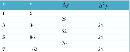
Problem 1:
Consider the function whose value of y for some equidistantly spaced values of x
x
1 3 5 7 9 11 [image:4.612.32.289.624.728.2]6 34 86 162 262 386
Table 1: Difference Table for Problem 1
x y
1 6
28
3 34 24
52
5 86 24
76
7 162 24
2 3 4 5
2 2 2 2 2
1 1 2 2
0 0
(
1)
(
1)
(
1)(
2)
(
1)(
2 )
...
2!
3!
4!
5!
y
y
y
y
y
=
y
+ ∆ +
u y
u u
−
∆
−+
u u
−
∆
−+
u u
−
u
−
∆
−+
u u
−
u
−
∆
−+
2 3 4 5
3 3 4 5
2 ( 2) 2 ( 1)( 2) ( 1)( 2)( 3) ( 1)( 2)( 3) ( 1)( 2)( 3)( 4) ...
2! 3! 4! 5!
y y y y
y=y− + + ∆ + +u y− u u+ ∆ − + +u u+ u+ ∆ − +u u+ u+ u+ ∆ − +u u+ u+ u+ u+ ∆ − +
5
2 3 4
2 2 2 2 2 3
1 2 2
0 1
(
1)
(
1)
(
1)(
2)
(
1)(
2 )
...
2!
3!
4!
5!
y
y
y
y
y
=
y
+ ∆ +
u y
−u u
+
∆
−+
u u
−
∆
−+
u u
−
u
−
∆
−+
u u
−
u
−
∆
−+
2 2 2 3
2 0 1 3 1 3 2
2 2
(
2)(
)
)
(
2)(
3)
(
1)
(
1)
(
1)
1
1
2
2
2!
2
3!
2
y
y
u
y
u
u
y
u y
u
u
u
y
u u
y
y
y
y
− − − − − −
− −
+
∆
+
+ ∆
+ ∆
+
+
+ ∆
+
− ∆
=
+ −
+
∆ +
+
+
∆
5 5
4 4
5 5
4 2
(
3)(
4)
(
1)(
2)
(
3)
(
1)
(
1)(
2)
(
1)(
2)
...
4!
2
5!
2
u
u
y
u
u
y
u
y
u
y
u u
+
u
+
+ ∆
−+ − ∆
−
u u
+
u
+
+
+ ∆
−+ −
− ∆
−
+
+
+
2
3
2
1
y
=
x
+
x
+
2
3
2
1
y
=
x
+
x
+
y
∆
2y
ISSN 2250-3153
100
9 262 24
124
11 386 24
148
13 534
Here we take 𝑥𝑥= 6,𝑥𝑥0= 7 ,ℎ= 2 , and 𝑢𝑢=𝑥𝑥−𝑥𝑥ℎ0=6−72 =−0.5
Actual value is: 𝑦𝑦(6) = 3(6)2+ 2(6) + 1 = 121
Gauss’s Forward Interpolation Formula gives
𝑦𝑦(6) = 162 + (−0.5)(100) +(−0.5)(−0.52! −1)(24)= 121
Gauss’s Backward Interpolation Formula gives:
𝑦𝑦(6) = 162 + (−0.5)(76) +(−0.5)(−0.5 + 1)(24)2! = 121
Stirling’s Interpolation Formula gives:
𝑦𝑦(6) = 162 + (−0.5)(100 + 76)2 +(−0.5)2! 2(24) = 121
Bessel’s Interpolation Formula gives:
𝑦𝑦(6) =162 + 2622 + (100) +(−0.5)(−20.5−1) = 121
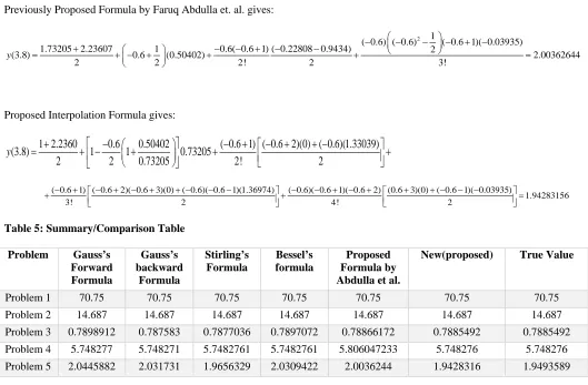
Previously Proposed Formula by Faruq Abdulla et. al. gives:
𝑦𝑦(6) =86 + 1622 + (76) +(−0.5)(−2!0.5 + 1) = 121
Proposed Interpolation Formula gives:
𝑦𝑦(6) =34 + 1622 + (52) +(−0.5 + 1)2! = 121
Problem 2:
The following table gives the value of the function for certain equidistant values of
1
0.5
2
−
−
24
24
2
+
1
0.5
2
−
+
24
24
2
+
0.5
76
1
1
2
52
−
+
( 0.5 2)(24) (0.5)24
2
−
+
−
3 2
2
7
3
y
=
x
−
x
+
x
−
x
x
0 1 2 3 4 5-3 3 11 27 57 107
3 2
2
7
3
ISSN 2250-3153
Table 2: Difference Table for Problem 3
x
0 -3
6
1 3 8
8 6
2 11 8
16 6
3 27 14
30 6
4 57 20
50
5 107
Here we take , and since , we have,
Actual value is:
Again, Gauss’s Forward Formula gives:
Gauss’s Backward Interpolation Formula gives
Stirling’s Interpolation Formula gives:
Bessel’s Interpolation Formula gives
3 2
2
7
3
y
=
x
−
x
+
x
−
∆
y
∆
2y
∆
3y
2.3
x=
x
0=
3
h=10
2.3 3
0.7
1
x
x
u
h
−
−
=
=
= −
3 2 3 2
2
7
3
(2.3)
2(2.3)
7(2.3) 3 14.687
y
=
x
−
x
+
x
− =
−
+
− =
(
2)
( 0.7) ( 0.7)
1 (6)
14
(2.3)
27 ( 0.7)(30) ( 0.7)( 0.7 1)
14.687
2!
3!
y
=
+ −
+ −
−
−
+
−
−
−
=
(
2)
( 0.7) ( 0.7)
1 (6)
14
(2.3)
27 ( 0.7)(16) ( 0.7)( 0.7 1)
14.687
2!
3!
y
=
+ −
+ −
−
+
+
−
−
−
=
(
2)
2
( 0.7) ( 0.7)
1
16 30
( 0.7)
6 6
(2.3)
27 ( 0.7)
(14)
14.687
2
2!
3!
2
y
=
+ −
+
+
−
+
−
−
−
+
=
1
0.7
0.7
( 0.7 1)(6)
57
27
1
0.7( 0.7 1) (14
20)
2
(2.3)
0.7
30
14.687
2
2
2!
2
3!
y
−
−
−
−
−
+
−
−
−
+
=
+ −
−
+
+
=
ISSN 2250-3153
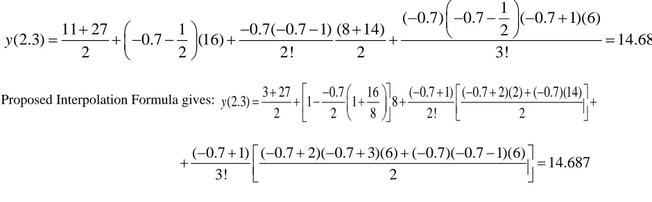
Previously Proposed Formula by Abdulla et. al. gives:
Proposed Interpolation Formula gives:
Problem 3:
[image:7.612.36.506.104.250.2]Consider the function for some equidistantly spaced values of
Table 3: Difference Table for Problem 4
x
0.7071
0.0589
0.7660 -0.0057
0.0539 -0.0007
0.8192 -0.0064
0.0468 0.8660
Here we take , and since , we have,
Actual value is:
Gauss’s Forward Interpolation Formula gives:
1
( 0.7)
0.7
( 0.7 1)(6)
11 27
1
0.7( 0.7 1) (8 14)
2
(2.3)
0.7
(16)
14.687
2
2
2!
2
3!
y
−
−
−
−
+
+
−
−
−
+
=
+ −
−
+
+
=
3 27 0.7 16 ( 0.7 1) ( 0.7 2)(2) ( 0.7)(14)
(2.3) 1 1 8
2 2 8 2! 2
y = + + − − + + − + − + + − +
( 0.7 1) ( 0.7 2)( 0.7 3)(6) ( 0.7)( 0.7 1)(6)
14.687
3! 2
− + − + − + + − − −
+ =
sin
y
=
x
x
sin
y
=
x
∆
y
2y
∆
3y
∆
0
45
0
50
0
55
0
60
0
52
x
=
x
0=
55
h
=
5
0
52 55
0.6
5
x
x
u
h
−
−
=
=
= −
0
sin 52
=
0.788010
x
0.7071 0.7660 0.8192 0.8660 0
45
50
055
060
0sin
ISSN 2250-3153
Gauss’s Backward Formula gives:
Stirling’s Interpolation Formula gives:
Bessel’s Interpolation Formula gives:
Previously Proposed Formula by Faruq Abdulla et al. gives:
Proposed Formula gives:
+
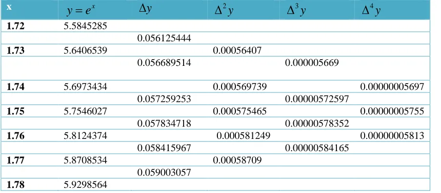
Problem 4:
The following table, gives the value of for certain equidistant values of . We find the value of x when
1.72 1.73 1.74 1.75 1.76 1.77 1.78
5.5845285 5.6406539 5.6973434 5.7546027 5.8124374 5.8708534 5.9298564
(
)
(
2)
0 2
0.0064
( 0.6) ( 0.6)
1 (0)
(52 )
0.8192 ( 0.6)(0.0468) ( 0.6) ( 0.6)
1)
0.7898912
2!
3!
y
=
+ −
+ −
−
−
−
+
−
−
−
=
(
)
(
2)
0
0.0064
( 0.6) ( 0.6)
1 ( 0.0007)
(52 )
0.8192 ( 0.6)(000539) ( 0.6)
0.6 1
0.787583
2!
3!
y
=
+ −
+ −
−
+
−
+
−
−
−
−
=
(
2)
2
0
0.0539 0.0468
( 0.6)
( 0.6) ( 0.6)
1
0.0007 0
(52 )
0.8192 ( 0.6)
( 0.0064)
0.7877036
2
2!
3!
2
y
=
+ −
+
+
−
−
+
−
−
−
−
+
=
2
1
0.6 0.6 ( 0.6 1)( 0.0007) 0.8660 0.8192 1 0.6( 0.6 1) ( 0.0064 0) 2
(52 ) 0.6 (0.0468) 0.7897072
2 2 2! 2 3!
y
− − − − − −
+ − − − − +
= + − − + + =
2
0
1
( 0.6) ( 0.6) ( 0.6 1)( 0.0007)
0.7660 0.8192 1 0.6( 0.6 1) ( 0.0057 0.0064) 2
(52 ) 0.6 (0.0539) 0.78866172
2 2 2! 2 3!
y
− − − − + −
+ − − + − −
= + − + + + =
0.7071 0.8192 0.6 0.0539 ( 0.6 1) ( 0.6 2)(0) ( 0.6)( 0.0064)
(2.3) 1 1 0.0589
2 2 0.0589 2! 2
y = + + − + + − + − + + − − +
0.6 1 ( 0.6 2)( 0.6 3)(0) ( 0.6)( 0.6 1)( 0.0007)
0.7885492
3!
2
−
+
−
+
−
+
+ −
−
− −
=
x
e
x
x
=
1.7489
x
x
ISSN 2250-3153
Table 4: Difference Table for Problem 2
x
1.72 5.5845285
0.056125444
1.73 5.6406539 0.00056407
0.056689514 0.000005669
1.74 5.6973434 0.000569739 0.00000005697
0.057259253 0.00000572597
1.75 5.7546027 0.000575465 0.00000005755
0.057834718 0.00000578352
1.76 5.8124374 0.000581249 0.00000005813
0.058415967 0.00000584165
1.77 5.8708534 0.00058709
0.059003057
1.78 5.9298564
Here we take , and since , we have,
Actual value is:
Now, Gauss’s Forward Interpolation Formula gives
Gauss’s Backward Interpolation Formula gives
Stirling’s Interpolation Formula gives:
x
y
=
e
∆
y
∆
2y
∆
3y
∆
4y
1.7489
x
=
x
0=
1.75
h
=
0.01
0
1.7489 1.75
0.11
0.01
x
x
u
h
−
−
=
=
= −
1.7489
5.748276093
x
y
=
e
=
e
=
(0.000575465)
(1.7489)
5.7546027 ( 0.11)(0.057834718) ( 0.11)( 0.11 1)
2!
y
=
+ −
+ −
−
−
+
(
2)
0.00000578352
(
2)
0.00000005755
( 0.11) ( 0.11)
1
( 0.11) ( 0.11)
1 ( 0.11 2)
5.748277091
3!
4!
+ −
+
−
+ −
+
− −
−
=
(0.000575465)
(1.7489)
5.7546027 ( 0.11)(0.057259253) ( 0.11)( 0.11 1)
2!
y
=
+ −
+ −
−
+
+
(
2)
0.00000572597
(
2)
0.00000005813
( 0.11) ( 0.11)
1
( 0.11) ( 0.11)
1 ( 0.11 2)
5.748271047
3!
4!
+ −
+
−
+ −
+
− −
+
=
2
(0.057259253 0.07834718)
( 0.11)
(1.7489)
5.7546027 ( 0.11)
(0.000575465)
2
2!
ISSN 2250-3153
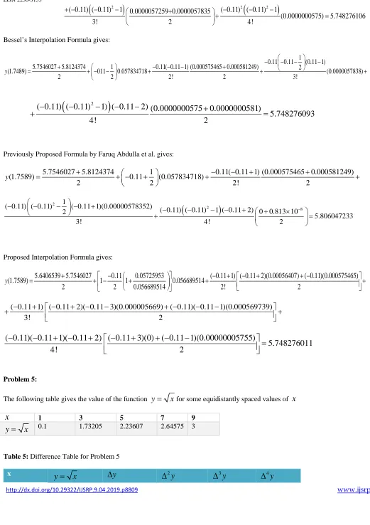
Bessel’s Interpolation Formula gives:
Previously Proposed Formula by Faruq Abdulla et al. gives:
Proposed Interpolation Formula gives:
Problem 5:
The following table gives the value of the function for some equidistantly spaced values of
1 3 5 7 9
[image:10.612.32.553.50.788.2]0.1 1.73205 2.23607 2.64575 3
Table 5: Difference Table for Problem 5
x
(
2)
2(
2)
( 0.11) ( 0.11) 1 0.0000057259+0.0000057835 ( 0.11) ( 0.11) 1
(0.0000000575) 5.748276106
3! 2 4!
+ − − − + − − −
=
1 0.11 0.11 (0.11 1) 5.7546027 5.8124374 1 0.11( 0.11 1) (0.000575465 0.000581249) 2
(1.7489) 011 0.057834718 (0.0000057838)
2 2 2! 2 3!
y
− − − −
+ − − − +
= + − − + + +
(
2)
( 0.11) ( 0.11)
1) ( 0.11 2) (0.0000000575 0.0000000581)
5.748276093
4!
2
−
−
−
−
−
+
+
=
5.7546027 5.8124374 1 0.11( 0.11 1) (0.000575465 0.000581249)
(1.7589) 0.11 (0.057834718)
2 2 2! 2
y = + + − + +− − + + +
(
)
2
2 8
1
( 0.11) ( 0.11) ( 0.11 1)(0.00000578352)
( 0.11) ( 0.11) 1 ( 0.11 2) 0 0.813 10 2
5.806047233
3! 4! 2
−
− − − − + − − − − +
+ ×
+ =
5.6406539 5.7546027 0.11 0.05725953 ( 0.11 1) ( 0.11 2)(0.00056407) ( 0.11)(0.000575465)
(1.7589) 1 1 0.056689514
2 2 0.056689514 2! 2
y = + + − − + + − + − + + − +
( 0.11 1) ( 0.11 2)( 0.11 3)(0.000005669) ( 0.11)( 0.11 1)(0.000569739)
3! 2
− + − + − − + − − −
+ +
( 0.11)( 0.11 1)( 0.11 2) ( 0.11 3)(0) ( 0.11 1)(0.00000005755)
5.748276011
4!
2
−
−
+ −
+
−
+
+ −
−
=
y
=
x
x
x
y
=
x
ISSN 2250-3153
1 1.0
0.73205
3 1.73205 -0.22803
0.50402 1.3694
5 2.23607 -0.09434 -0.03935
0.40968 1.33039
7 2.64575 1.23605
1.64573
9 3
Here we take , and since , we have,
Actual value is:
Gauss’s Forward Interpolation Formula gives:
Gauss’s Backward Interpolation Formula gives:
Stirling’s Formula Interpolation gives:
Bessel’s Interpolation Formula gives:
3.8
x
=
x
0=
5
h
=
2
0
3.8 5
0.6
2
x
x
u
h
−
−
=
=
= −
3.8
1.949358869
y
=
x
=
=
(
2)
( 0.6) ( 0.6)
1 (1.33039)
0.09434
(3.8)
2.23607 ( 0.6)(0.40968) ( 0.6)( 0.6 1)
2!
3!
y
=
+ −
+ −
−
−
−
+
−
−
−
+
(
2)
( 0.6) ( 0.6)
1 ( 0.6 2)( 0.03935)
2.044588174
4!
−
−
−
−
−
−
+
=
(
2)
( 0.6) ( 0.6)
1 (1.36974)
0.09434
(3.8)
2.23607 ( 0.6)(0.50402) ( 0.6)( 0.6 1)
2!
3!
y
=
+ −
+ −
−
+
−
+
−
−
−
+
(
2)
( 0.6) ( 0.6)
1 ( 0.6 2)( 0.03935)
2.03173096
4!
−
−
−
−
+
−
+
=
(
2)
2
( 0.6) ( 0.6)
1
0.50402 0.40968
( 0.6)
1.3694 1.33039
(3.8)
2.23607 ( 0.6)
( 0.22803)
2
2!
3!
2
y
=
+ −
+
+
−
−
+
−
−
−
+
+
(
)
2 2
( 0.6)
( 0.6)
1 ( 0.03935
1.96563288
4!
−
−
−
−
+
=
1
0.6
0.6
( 0.6 1)
2.64575 2.23607
1
0.6( 0.6 1) 0.09434 1.23605
2
(3.8)
0.6
(0.40968)
(1.33039)
2
2
2!
2
3!
y
−
− −
− −
+
−
− − −
+
=
+ − −
+
+
+
ISSN 2250-3153
Previously Proposed Formula by Faruq Abdulla et. al. gives:
Proposed Interpolation Formula gives:
[image:12.612.33.562.125.472.2]
Table 5: Summary/Comparison Table
Problem Gauss’s Forward Formula
Gauss’s backward
Formula
Stirling’s Formula
Bessel’s formula
Proposed Formula by Abdulla et al.
New(proposed) True Value
Problem 1 70.75 70.75 70.75 70.75 70.75 70.75 70.75
Problem 2 14.687 14.687 14.687 14.687 14.687 14.687 14.687
Problem 3 0.7898912 0.787583 0.7877036 0.7897072 0.78866172 0.7885492 0.7885492 Problem 4 5.748277 5.748271 5.7482761 5.7482761 5.806047233 5.748276 5.748276 Problem 5 2.0445882 2.031731 1.9656329 2.0309422 2.0036244 1.9428316 1.9493589
Error Analysis:
We shall now carry out an error analysis using the concept of mathematical norm, to determine which numerical method of interpolation from Table 5 above, is best.
Table 6: Comparing the Actual Values of the functions and the values obtained using Gauss’s Forward Interpolation Formula:
Actual(A) Gauss's Forward(P1) K1 = |A-P1| %Error
70.75 70.75 0 0
14.687 14.687 0 0
0.788549 0.7898912 0.001342 0.170186
5.748276 5.748277 9.98E-07 1.74E-05
(
2)
( 0.6) ( 0.6)
1) ( 0.6 2)
0.03935 0
2.03094224
4!
2
−
−
−
−
−
−
+
+
=
2 1
( 0.6) ( 0.6) ( 0.6 1)( 0.03935)
1.73205 2.23607 1 0.6( 0.6 1) ( 0.22808 0.9434) 2
(3.8) 0.6 (0.50402) 2.00362644
2 2 2! 2 3!
y
− − − − + −
+ − − + − −
= + − + + + =
1 2.2360 0.6 0.50402 ( 0.6 1) ( 0.6 2)(0) ( 0.6)(1.33039)
(3.8) 1 1 0.73205
2 2 0.73205 2! 2
y = + + − − + + − + − + + − +
( 0.6 1) ( 0.6 2)( 0.6 3)(0) ( 0.6)( 0.6 1)(1.36974) ( 0.6)( 0.6 1)( 0.6 2) (0.6 3)(0) ( 0.6 1)( 0.03935)
1.94283156
3! 2 4! 2
− + − + − + + − − − − − + − + + + − − −
+ + =
ISSN 2250-3153
1.949359 2.0445882 0.095229 4.88516
= 0.096572
= 0.095239
[image:13.612.30.352.367.471.2]= 0.095229
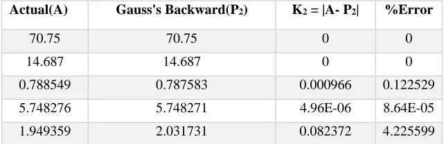
Table 7: Comparing the Actual Values of the functions and the values obtained using Gauss’s
Backward Interpolation Formula
Actual(A) Gauss's Backward(P2) K2 = |A- P2| %Error
70.75 70.75 0 0
14.687 14.687 0 0
0.788549 0.787583 0.000966 0.122529
5.748276 5.748271 4.96E-06 8.64E-05
1.949359 2.031731 0.082372 4.225599
=0.083343
=0.082378 1 1
0.7898912
5.748277009
2.
| 70.5 70.5 |
|14.687 14.687 |
| 0.7885492
|
|
4
044588
5.7 827601
|
|1.9
49358
87
1
7 |
4
K
=
−
+
−
+
−
+
−
+
−
2 2 2
1 2 2 2
(| 70.5
70.5 |)
(| 14.687 14.687 |)
(| 0.7885492
0.7898912
|
5.748277009
2.0
)
(| 5.748
27601
|)
(|
1.949
35887
445
8
8
1 4
7
|)
K
=
−
+
−
+
−
+
+
−
+
−
1
0.7898912
5.748277009
2.04458
| 70.5 70.5 |
|14.687 14.687 |
| 0.7885492
|
| 5.748276
8
01
|
max
|1.94935887
174
|
K
∞=
−
+
−
+
−
+
−
+
+
−
2 1
| 70.5 70.5 |
|14.687 14.687 |
| 0.7885492 0.787583 |
| 5.74827601 5.748271047 |
|1.94935887 2.03173096 |
K
=
−
+
−
+
−
+
−
+
+
−
(
) (
) (
)
(
)
2 2 2
2 2 2
| 70.5
70.5 |
| 14.687 14.687 |
| 0.7885492
0.787583 |
| 5.74827601 5.748271047 |
K
=
−
+
−
+
−
ISSN 2250-3153
[image:14.612.30.353.149.262.2]= 0.082372
Table 8: Comparing the Actual Values of the functions and the values obtained using Stirling’s Formula:
Actual(A) Stirling’s Formula(P3) K3 = |A- P3| %Error
70.75 70.75 0 0
14.687 14.687 0 0
0.788549 0.7877036 0.000846 0.107235
5.748276 5.7482761 9.50E-08 1.65E-06
1.949359 1.9656329 0.016274 0.834839
= 0.01712
= 0.016296
= 0.016274
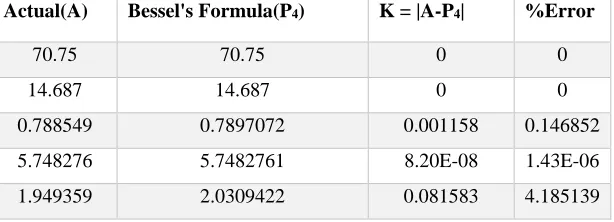
Table 9: Comparing the Actual Values of the functions and the values obtained using Bessel’s Interpolation Formula:
Actual(A) Bessel's Formula(P4) K = |A-P4| %Error
70.75 70.75 0 0
14.687 14.687 0 0
0.788549 0.7897072 0.001158 0.146852
5.748276 5.7482761 8.20E-08 1.43E-06
1.949359 2.0309422 0.081583 4.185139
[image:14.612.35.342.592.703.2]2
| 70.5 70.5 |
|14.687 14.687 |
| 0.788
7
5492 0.787583 |
max
| 5.74827601
5.748271
047 |
|
1.9493588
7
2.031 309
6
|
K
∞=
−
+
−
+
−
+
+
−
+
−
3 1
0.7877036
5.748276106
1
| 70.5 70.5 |
|14.687 14.687 |
| 0.7885492
|
| 5.7
2
4827601
|
|
1.
9
49
3
5887
.
9
6
5
6
3
88
|
K
=
−
+
−
+
−
+
−
+
+
−
(
) (
) (
)
(
) (
)
2 2 2
3 2 2 2
0.7877036
5.748276106
1.94935887 1.96563
| 70.5
70.5 |
|14.687 14.687 |
| 0.7885492
|
| 5.74
827601
|
|
2
8
8
|
K
=
−
+
−
+
−
+
−
+
−
3
| 70.5 70.5 |
|14.687 14.687 |
| 0.788
6
5492 0.787583 |
max
| 5.74827601
5.748271
047 |
|
1.9493588
7
1.965 328
8
|
K
∞=
−
+
−
+
−
+
+
−
+
−
ISSN 2250-3153
= 0.082741
= 0.081592
[image:15.612.30.426.306.414.2]
= 0.081583
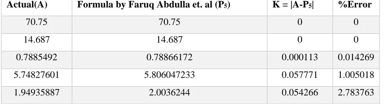
Table 10: Comparing the Actual Values of the functions and the values obtained using the proposed interpolation formula by Faruq Abdulla et al.
Actual(A) Formula by Faruq Abdulla et. al (P5) K = |A-P5| %Error
70.75 70.75 0 0
14.687 14.687 0 0
0.7885492 0.78866172 0.000113 0.014269
5.74827601 5.806047233 0.057771 1.005018
1.94935887 2.0036244 0.054266 2.783763
= 0.112149
=0.079261
= 0.057771
Table 11: Comparing the Actual Values of the functions and the values obtained using the New (proposed) Interpolation Formula:
Actual(A) Proposed Formula (P6) K = |A-P6| %Error
4 1
0.7897072
5.748276093
2
| 70.5 70.5 |
|14.687 14.687 |
| 0.7885492
|
| 5.7
2
4827601
|
|
1.
9
49
3
5887
.
0
3
0
9
4
24
|
K
=
−
+
−
+
−
+
−
+
+
−
(
) (
) (
)
(
) (
)
2 2 2
4 2 2 2
0.7897072
5.748276093
1.94935887
2.03094
| 70.5
70.5 |
|14.687 14.687 |
| 0.7885492
|
| 5.74
827601
|
|
2
2
4
|
K
=
−
+
−
+
−
+
−
+
−
4
0.7897072
5.748276093
1.94935887 2.0309
| 70.5 70.5 |
|14.687 14.687 |
| 0
2
.7885492
|
max
| 5.74827601
|
|
4
2
4 |
K
∞=
−
+
−
+
−
+
+
−
+
−
5 1
0.78866172
5.806047233
2.003
| 70.5 70.5 |
|14.687 14.687 |
| 0.7885492
|
| 5.74827601
|
|1.94935887
6244 |
K
=
−
+
−
+
−
+
−
+
+
−
(
) (
) (
)
(
) (
)
2 2 2
5 2 2 2
0.7886617
2
|
2
5.806047233
7
1.94935887
.0036
70.5
70.5 |
|14.687 14.687 |
| 0.78854
4
92
|
| 5. 4827
601
|
|
2 4
|
K
=
−
+
−
+
−
+
−
+
−
5
0.7885492
5.748276011
1.94935887 1.9428
| 70.5 70.5 |
|14.687 14.687 |
| 0
5
.7885492
|
max
| 5.74827601
|
|
3
1
6 |
K
∞=
−
+
−
+
−
+
+
−
+
−
ISSN 2250-3153
70.75 70.75 0 0
14.687 14.687 0 0
0.788549 0.7885492 0 0
5.748276 5.748276 0 0
1.949359 1.9428316 0.006527 0.334844
= 0.006527
= 0.006527
[image:16.612.32.374.54.145.2]= 0.006527
Table 11: Error Comparison
Norm Gauss’s
Forward
Gauss’s Backward
Stirling’s Formula
Bessel’s Formula
Formula by Abdulla et al.
Proposed Formula 0.096572 0.083343 0.01712 0.082741 0.112149 0.006527
0.095239 0.082378 0.016296 0.081592 0.079261 0.006527
0.095229 0.082372 0.016274 0.081583 0.05771 0.006527
4. CONCLUSION
This paper is on a New (proposed) Formula for Interpolation and Comparison with existing models of interpolation, using the concept of mathematical norm. The new model given in equation (8), is center based i.e. when the value to be interpolated is from the centre region in a given data set. The New formula was obtained by retreating the subscript in Gauss’s Forward Interpolation Formula by two units and replacing u by u+2, then the resulting equation was added to the Gauss’s Backward Interpolation Formula and the mean taken to obtain the New (proposed) Model. The New (proposed) Formula for Interpolation was then tested against the existing Formulae which includes: Gauss’s Forward Interpolation Formula, Gauss’s Backward Interpolation Formula, Stirling’s Interpolation
6 1
0.7885492
5.748276011
1
| 70.5 70.5 |
|14.687 14.687 |
| 0.7885492
|
| 5.7
1
4827601
|
|
1.
9
49
3
5887
.
9
4
2
8
3
56
|
K
=
−
+
−
+
−
+
−
+
+
−
(
) (
) (
)
(
) (
)
2 2 2
6 2 2 2
0.7885492
5.748276011
1.94935887 1.94283
| 70.5
70.5 |
|14.687 14.687 |
| 0.7885492
|
| 5.74
827601
|
|
1
5
6
|
K
=
−
+
−
+
−
+
−
+
−
6
0.7885492
5.748276011
1.94935887 1.9428
| 70.5 70.5 |
|14.687 14.687 |
| 0
5
.7885492
|
max
| 5.74827601
|
|
3
1
6 |
K
∞=
−
+
−
+
−
+
+
−
+
−
1
−
norm
2
−
norm
norm
ISSN 2250-3153
Formula, and Bessel’s Interpolation Formula and a Formula previously proposed by Faruq Abdulla et al. The results obtained, was analyzed using the concept of Mathematical Norm, and it was discovered that the New model has the minimum errors with respect to 1-norm, 2-norm and infinity-norm. Therefore, the New (proposed) model, is best for central difference based Interpolation
REFRENCES
Abdulla, F., Hossan, M. & Rahman, M. (2004). “A New (Proposed) Formula for Interpolation and Comparison with Existing Formula for Intepolation”. Journal of Mathematical Theory and Modeling. 4(4) , 33-48, 2004.
Akima, H. (1970). “A new method of interpolation and smooth curve fitting based on local procedure”. Journal of the ACM (JACM) 17(4), 589-602, 1970.
Bater, C.W. & Coops,N.C. (2009). ”Evaluating Errors Associated with Lidar-derived DEM Interpolation” Computer & Geoscience 35(2), 289-300, 2009.
Conte, S.D. & Carl de Boor (1980). Elementary Numerical Analysis, 3rd edition, McGraw-Hill, New York, USA
Das, B., & Chakrabarty, D. (2016). Lagranges Interpolation Formula: Representation of Numerical Data by a Polynomial Curve. International Journal of Mathematics Trend and Technology, 23-31.
Das, B., & Chakrabarty, D. (2016). Newton’s backward interpolation: Representation of numerical data by a polynomial curve. IJAR, 2(10), 513-517.
Das, B., & Chakrabarty, D. (2016). Newton’s Divided Difference Interpolation Formula: Representation Numerical Data by a Polynomial Curve. International Journal of Mathematics Trend andTechnology, 26-32.
Endre Suli, E., & Mayers, d. (2003). An Introduction to Numerical Analysis, Cambridge, UK.
Fritsch, F.N., & Carlson, R.E. (1980). “Monotone Piecewise Cubic Interpolation”. SAIM Journal of Numerical Analysis 17(2) 238-246, 1980.
Garnero, G., & Godone, D. (2013). Comparisons between different interpolation techniques. Proceedings of the international archives of the photogrammetry, remote sensing and spatial information sciences XL-5 W, 3, 27-28.
Liu, G.R., Zhang, J., Li, H., Lam, K.Y. & Kee , B.B. T (2006). “Radial Point Interpolation based on Finite Difference Method for Mechanic Problems” International Journal for Numerical Methods in Engineering 68(7), 728-754, 2006.
Kendall E. Atkinson (1989). An Introduction to Numerical Analysis, 2nd edition, John Wiley & Sons, New York.
Muthumalai, R. K. (2008). New Iterative Methods for Interpolation, Numerical Differentiation and Numerical Integration. arXiv preprint arXiv:0809.1643.
Muthumalai, R. K., & Uthra, G. (2014). • A NOTE ON POLYNOMIAL INTERPOLATION FORMULAE. International Journal of Mathematical Archive EISSN 2229-5046, 5(7).
Reuter, H.I., Nelson,A. & Jarvis, A. (2007). “An Evaluation of Void-Filling Interpolation Methods for STRM Data”. International Journal of Geographical Information Science 21(9), 983-1008, 2007.