Dynamical Modelling and Positioning Control Simulation of a Spherical Robot Driven by Three Omnidirectional Wheels

2017 2nd International Conference on Computational Modeling, Simulation and Applied Mathematics (CMSAM 2017) ISBN: 978-1-60595-499-8

Dynamical Modelling and Positioning Control Simulation of a Spherical

Robot Driven by Three Omnidirectional Wheels

Yong-hua HUANG

*

, Gan-min ZHU, Chang-sheng WANG and Hao HUANG

School of Mechanical and Electrical Engineering, Guilin University of Electronic Technology, Guilin, China, 541004

*Corresponding author

Keywords: Spherical robot, Omnidirectional wheels driving, Dynamical model, Position regulation.

Abstract. In this paper, we concerned on the dynamical modelling and the position control problem for a novel spherical robot which was driven by three omnidirectional wheels. We first introduce the mechanism of our spherical robot. And then considering the noholonomic constraints of the shell contacting with the omnidirectional wheels and the shell contacting with the ground, we developed a nonlinear dynamical model for the system by use of Chaplygin equation. With the model, we suggested that the robot was an under-actuated system which consists of six independent velocities and three driving-torque inputs. By linearized the position variables of the shell, we designed a controller to regulate the position of the system according to the Theorem of Partial Feedback Linearization. Numerical simulations were exploited to show the effectiveness of our controller.

Introduction

Driving mechanism is one of the most critical factors in determining the performance of a spherical robot. In the past four decades, several kinds of mechanism have been used to design a spherical robot. Considering the working principle differences of the driving mechanism, at present, the spherical robot can be sorted into two types, that is, the eccentric moment driving spherical robot and the angular momentum driving spherical robot.

For the former, the working principle was summarized as that the driving mechanism of the spherical robot force the COG (center of gravity) of the system deviating from the vertical sphere center line, in this case, the balance of the system is destroyed, and under the action of gravity moment the sphere shell then run on the ground. In [1], A. Halme et al. proposed a spherical robot with a single wheel on the bottom of the spherical shell. He believed when the wheel rolls along the inner surface of the shell, an eccentric moment would be aroused, so the shell began running at once. In [2], Ranjan Mukhejee et al. presented a spherical robot that was driven by four moving masses. Mukhejee gave the idea when the masses move on their individual leadscrew along the sphere diameter, the COM (center of mass) of the system should be changed, and as a result, the shell would begin to roll. In [3,4], There are similar scheme. In [5], J Alves et al. considered a four wheels vehicle in his spherical robot. Alves suggested that the running vehicle on the bottom of the inner shell could give a moment to drive the shell running. In [6], Zhan et al. exploited an omnidirectional as steering wheel and a longitudinal driving wheel to drive the sphere shell. Zhan addressed that if the exact rotations of the two wheels were perform, the shell should run in all direction. Similar to Zhan, in [7], Wang discussed a spherical robot of two omnidirectional wheels on two orthogonally axis. In [8], Sun et al. proposed a weight-pendulum of two degree of freedom in their spherical robot. Sun argued that, as the pendulum could be driven to swing in all directions, the robot then might run in omnidirection. In [9], Zhao et al. presented a spherical robot with two coaxial eccentric masses. Zhao believed when the masses run with different acceleration and velocity, the robot should consequently move in all direction. The similar mechanism was also proposed in [10].

the running shell and the ground, with the principle of the angular momentum conservation, the shell would rotate reverse to that of the running rotor. Furthermore, if we alternated the speed and direction of the rotating rotor, the omnidirectional motion of the spherical robot then could be gotten. In [11], Toshiaki Otani et al. developed a spherical robot driven by a three axis mechanical gyroscope. The robot’s gyroscope was fixed on a gimbal inside the sphere, and when it rotated with high speed, they believed, there would be a counter moment that can drive the shell to run definitely. In [12], V. Joshi et al. proposed a spherical robot with double rotors which shared the similar principle in [11].

By now, there is a trend that the spherical robot of the former showed more advantage than the spherical robot of the latter, e.g., more steering flexibility, lower speed of the driving mechanism. Especially, the robot developed recently in [9] and [10] that used omnidirectional wheels, have exhibited a great deal of extinguished performance. For this reason, the former is still attracting in spherical robot research. Furthermore, utilizing the omnidirectional wheels to develop a driving mechanism for a spherical robot might be a promising technology in the future.

In this paper, we consider a new type of spherical robot driven by three inner omnidirectional wheels. At first, we introduce the mechanical structure of our spherical robot in detail; and next, we develop a dynamical model for the robot system by using Chaplygin equation; moreover, we design a position regulating controller by the Theorem of Partial feedback Linearization for the system and perform a simulation to testify the effectiveness of our derivation.

Mechanism and Working Principle

The spherical robot in [9] and [10] were designed with one wheel contacting with their shell, which might restrict the driving capability of the system, thus we use three omnidirectional wheels to improve our robot’s performance.

Mechanical Structure

The structure of the system is shown in Figure 1~Figure 2.

Figure 1. Principle prototype of our spherical robot. Figure 2. The schematic diagram of our spherical robot.

Working Principle

The working principle of our robot is as follows:

At the beginning, the three motors drive the omnidirectional wheels to run regulated by a given law. Simultaneously, the running wheels would synthesize a couple to propel the shell to roll via the contacting friction. And in other word, if we control the rotational velocity and direction of the wheels, we could drive the sphere shell in all direction.

After the omnidirectional wheels being driven, because the three wheels are all fixed on the inner platform, there should be a reaction couple acting on the platform by the omnidirectional wheels. With the help of the four free-running ball wheels, the reaction couple would drive the platform to rotate about the geometric center of the shell.

Moreover, if we configure the COG of the platform in different position, the support platform could work either as a rotor of high speed rotating or a pendulum of low speed swinging.

Dynamics

For facilitating our analysis, we assume that our robot had the following characteristics:

Assumption 1: the omnidirectional wheels, the shell and the support platform are all rigid body.

Assumption 2: the joints between the platform and the omnidirectional wheels are frictionless.

Assumption 3: the sphere shell rolls on a horizontal plane without slipping; the omnidirectional wheels run on the inner surface of the shell without slipping.

Additionally, we represent the support platform asB₁, the shell as B₂, and the omnidirectional

wheels as B_i(i3, 4,5). The coordinates of the robot are set up as follow:

 Oe e e_{1 2 3}{0}is the global coordinate system fixed on the ground;

 (1) (1) (1) 1 1 2 3

O e e e {1} is the coordinate system of the inner supporting platformB₁ and its origin is

the geometric center of the sphere shellB₂;

 (2) (2) (2) 2 1 2 3

O e e e {2}is the coordinate system of the shellB₂ and its origin is the same as{1}

 ( ) ( ) ( ) 1 2 3

i i i

i

O e e e {i} (i3, 4,5) is the coordinate system of the omnidirectional wheelB_i and the origin locates at its geometric center.

Kinetic Model

We represent e_i( )j (i1, 2,3, j1, 2,3, ) as the ith base vector of coordinate{ }j , s_i sin( )q_i ,

cos( )

i i

c  q (i1, 2, ), and q_i(i1, 2,3) as the ith Eular angular rate of B₁. Because the sphere

shell rolls on a horizontal plane, the angular velocity ofB₁ can be given as:

(1) (1) (1) (1)

1 ( 3 2 2 3 1) 1 ( 2 1 3) 2 ( 2 3 1 3 2) 3

B  c q c s q  s q q  c c q s q

ω e e e . (1) Similarly, the angular velocity of B₂ can be given as:

(2) (2) (2) (2)

2 5 1 5 6 2 ( 4 5 6) 3

B q c q  q s q

ω e e e , (2) where (i4,5, 6) is the (i3)th angular rate of the sphere shell.

Considering B_i(i3, 4,5) rotate about B₁, we can get the angular velocity of B_i(i3, 4,5) as:

( ) (1) ( ) 1 1 ( 4) 3

j j j

Bj  B q j

ω R ω e ( j3, 4,5), (3)~(5)

where jR_i( ,i j1, 2, ) denotes the rotation transform matric from { }i to { }j , and q_i(i7,8,9)

denotes the angular rate of B_i(i3, 4,5), respectively.

(0) 0 (2) (0) 2 ( 2 2) 0

o  B  

υ R ω R , (6) where R(0) is the position vector of the shell-ground contacting point P in {0}. If we assume

(0) (0) (0)

2 1 2

o x y

υ e e (x,y) denote the longitudinal and the lateral velocity of the geometric center ofB2, respectively) and consider the first two items in (6), we would get:



 



5 4 4 /

q  s x c y lr , q6 



c x4 s y4

 

/ (lr c) 5



, (7)~(8)

where l is the distance between the geometer center of B₂ and that of B_i (i3, 4,5); ris the radius of the omnidirectional wheel.

Similarly, we investigate the velocities of the contact point between B₂ and B_i(i3, 4,5), then get

5

(6 5) (6 4) (6 3) 4 (6 5 ) (4 ) 3

i i i i i j j

j

q g _ x g _ y g _ q g _{ } q _



   



(i1, 2,3), (9)~(11)

in (9)~(11), g_j( j1, 2,3, ,18) is a function relating to q_i(i1, 2,3, 4,5).

Due to the velocity of the geometric center of B₂ satisfy υ_C(0)₂ υ_o(0)₂ , under the principle of the

relative motion we will get the velocity of B_i( ,i j1, 2, ,5) as:

(1) 1 (0) (1) (1)

1 0 2 1 1

C  o  B  C

υ R υ ω l , υ_Ck(1) 1R υ_{0 o}(0)₂ ω_B(1)₁



l_ok(1)1R l_{i Ci}( )k



(k 3, 4,5), (12)~(15)

where l_Ci( )i (i1,3, 4,5) denotes the position vector in { }i from the center of B₂ to that of B_i;

(1)

oi

l (i3, 4,5) is the position vector in {1} from the geometric center of B₂ to that of

i

B(i3, 4,5).

According to ( )j Bi

ω ( ,i j1, 2, ,5) in (1)~(5) and ( )k Ci

υ (i1, 2, ,5;k0,1) in (12)~(15), we can calculate the system’s kinetic energy as:

5

( ) ( ) ( ) ( ) 1

(( _Bij )T _Bi( _Bij ) ( _Cik )T _Bi( _Cik )) / 2

i

T M







ω J ω  υ υ , (16)

where J_Bi(M_i)(i1, 2, ,5) is the inertial matric(mass matrix) of B_i(i1, 2, ,5), respectively.

By substituting (7)~(11) into T , we will get another form of the kinetic energy T .

Dynamic Model

The external force acting on our spherical robot consist of the driving torque of B_i(i3, 4,5) and

the gravity. We consider the COM of B_i(i1,3, 4,5), which can be represented as:





(1) (1) (1) 1 (3) (1) 1 (4) (1) 1 (5) 1 1 3( 3 3 3) 4( 4 4 4) 5( 5 5 5) /

C  m C m o  C m o  C m o  C mt

l l l R l l R l l R l , (17)

where m_t m₁m₃m₄m₅. If we defined h 1R li C(1)[3] ( ( )[3] is the 3rd item of the vector),

we will find h is the function of q_i(i2,3). And if we take the first time derivative of h, we will get:

1 2 2 3

h f q  f q , (18)

in (18), f_i(i1, 2) denotes the explicit function of q_i (i2,3) and m_j( j1,3, 4,5). With (18),

we define τ_g



0 _g2 _g3



T, in which gk m g ft _k_1 (k 2,3).

Moreover, according to (9)~(11), we define a transform matric:

 

3 6

ij

g

 _

R . Consequently, the

g   

Q Q R τ , (19)

where Q



0 0 0 ₇ ₈ ₉



T, _i(i7,8,9) is the driving torque of B_j( j3, 4,5). Considering the following form of Chaplygin equation

, ,

1 1

B B

Q

d T T T

dt q q q q q q

 

     

 

    

 



 

  

 

 

 _  _  _

 

 







_   _  , (20) where T is the kinetic energy and T is the kinetic energy by substituting noholonomic constraints intoT ; B_{   ,} is the th coefficient of the th noholonomic constrain; q_ and

q_ are the generalized coordinates of the system;  and  are the numbers of the independent

generalized coordinates and the noholonomic constrains; Q_ is the th generalized force of the system.

We can get the system’s dynamics:

( ) _  ( , _) _ ( )

D q q C q q q G q Q, (21)

in (21), D q( )6 6 , C q q( , _)6 6 , and G q( )6 1 denote the inertia, centripetal-Coriolis,

and gravity terms; q_ and q are two kinds of generalized coordinates, which are represented as

follow:



4 7 8 9



T

x y q q q q

 

q and



1 2 3 4 5



T

q q q q q



q .

Equation (21) indicates our robot is an under-actuated system with six independent velocities, and the longitudinal displacement and lateral displacement (x,y) of the geometric center ofB₁, the

yaw angle (q₄) of B₁ are under-actuated; there are three driving inputs in q_i(i7,8,9), so we

could regulate control-force _i(i7,8,9) to control the trajectory (x,y,q₄) of the sphere shell.

Positioning Controller

Our control objective is to regulate the position of the COM of the sphere shell to a constant desired

setpoint:



4

 

0



T T

d d

x y q  x y . Accordingly, we should define an error signal as:



1 2 3 4 5 6

 

4 4



T T

d d d d

e e e e e e xx xx yy yy q q

, (22) We investigate the first three items of the dynamical model (Seeing Eq.(21)):

1( ) 1( ) 1( , )

u u a a  

D q q D q q F q q 0

, (23)

where q_u 



x y q₄



T, q_a 



q₇ q₈ q₉



T, and F q q₁( , _)3 1 is the first three items of



C q q q( , _) _ G q( )



, D_u1( ),q D_a1( )q 3 3 are a sub-matric ofD q( ). Then we will get



 

1



1( ) 1( , ) 1( )

a a u u

  



  

q D q F q q D q q . (24)

Substituting (24) into the last three items of the dynamical model, we will get:







1







1

2( ) 2( ) 1( ) 1( ) 2( ) 1( ) 1( , ) 2( , )

u a a u u a a   a

 

   

D q D q D q D q q D q D q F q q F q q τ , (25)

whereF q q₂( , _)3 1 is the last three items of



C q q q( , _) _ G q( )



, andD_u2( ),q D_a2( )q 3 3 are the corresponding sub-matric ofD q( ). If we define q_u v, we will get the input torque as:







1







1

2( ) 2( ) 1( ) 1( ) 2( ) 1( ) 1( , ) 2( , )

a u a a u a a  

 

   

where the virtual control law are defined as:v k ep 1k ed 1, 1



1 3 5



T

e e e



e , 1



2 4 6



T

e e e



e ,

3 3

,

p d

 

k k , and k_p diag k



_p1 k_p2 k_p3



, kd diag k



d1 kd2 kd3



, kpi, kdi(i1, 2,3) are

positive constant control gains. With (26), we will obtain the following theorem:

Theorem: The controller (26) ensures the system:



_{4 4}



0 ( ) ( ) ( ) ( ) ( ) ( )

T

t x t x t y t y t q t q t 

limit



xd 0 yd 0 0 0



T, where





T

d d

x y is the desired position of the COM of the sphere shell. Proof:In orderto prove the Theorem, firstly, we define

1 u ud  u 

e q q q v, (27)

where q_ud 



x y q₄

 

T  0 0 0



T. According to (27), we will obtain:

1 d 1 p 1 

e k e k e 0, (28)

In (28), if we set suitable k_d,k_p, we will get: _{1 1 1}

0 ( ) , 0 ( ) , 0 ( )

t t  t t  t t 

limit e 0 limit e 0 limit e 0. That is





0 ( ) , 0 ( ) 0

T

u u d d

t  t  t  t  x y

limit q 0 limit q . (29)

After substituting (29) into (23), we can obtain the zero dynamics of the robot system:

1( ) 1( , )

a a  

D q q F q q 0. (30)

Considering (30) around balanced point (q₁0,q₂ arcsin( 3 / 3), q₃  arcsin( 2 / 2)), we will obtain: F q q₁( , _)0 , F q q₂( , _)0 ; g₄g₆0, g₅  (in which  is a constant),

10 12

g  g , g₁₁0, g₁₆g₁₈ g₁₇/ 2. As a result, we can utilize (30) to show that q_a 0, and

utilize (26) to show τ_a 0. Eventually, we can get that q_a γ(where γ3 1 is a constant vector).

With (7)~(11), it is clear that q₁c,q₂q₃q₅q₆0 (where c is a constant). So we can get



1 2 3 4 5 6

 



0

( ) ( ) ( ) ( ) ( ) ( ) T 0 0 0 0 0 T

t

q t q t q t q t q t q t c

 

limit . (31)

Summarily, with (29) and (31), we can conclude that is the end of our proof.

Control Simulation

We preset the desired objective as:



x_d y_d



T  



1 e0.01t 0



T( )m , q_4d 0(rad). Considering the controller (26), we tuned the virtual control gains until there a better performance was achieved:

1 0.022

p

k  ,kp2 0.015, kp30.010, kd10.025, kd20.020, kd30.010.

The structural parameters of our system were set as: r0.06( )m ; l0.25( )m ;L₁0.20( )m (the

distance between the shell’s center and the COG of the platform); L₂0.25( )m (the distance

between omnidirectional wheel’s center and COG); m₁17.57(kg)

( m₂2.87(kg) , m₃0.45(kg) );





1

2

0.780 0.780 0.780 ( · )

B k

J diag gm , 2





2

0.130 0.130 0.130 ( · )

B k

J diag gm , J_B3 diag





2

0 100 200 300 400 500 600 700 800 0 0.5 1 t/s x/ m x x_d

0 100 200 300 400 500 600 700 800 -1

0 1x 10

-13 t/s y/ m y y_d

0 100 200 300 400 500 600 700 800 0 0.5 1 t/s x/ m x x d

0 100 200 300 400 500 600 700 800 -1

0 1x 10

-13 t/s y/ m y y d

[image:7.595.80.513.72.163.2]

a) The position coordinate ofx-axis b) The position coordinate ofy-axis

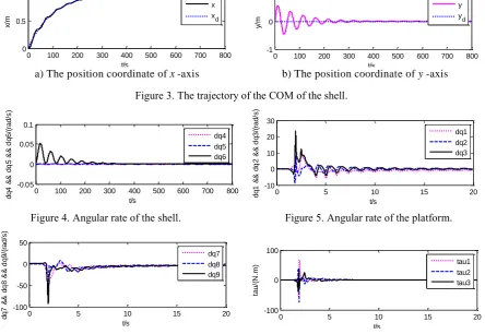
Figure 3. The trajectory of the COM of the shell.

0 100 200 300 400 500 600 700 800 -0.05 0 0.05 0.1 t/s d q 4 & & d q 5 & & d q 6 /( ra d /s ) dq4 dq5 dq6

0 5 10 15 20

-10 0 10 20 30 t/s d q 1 & & d q 2 & & d q 3 /( ra d /s ) dq1 dq2 dq3

Figure 4. Angular rate of the shell. Figure 5. Angular rate of the platform.

0 5 10 15 20

-100 -50 0 50 t/s d q 7 & & d q 8 & & d q 9 /( ra d /s ) dq7 dq8 dq9

0 5 10 15 20

-100 0 100 t/s ta u /( N .m ) tau1 tau2 tau3

Figure 6. Angular rate of the omnidirectional wheels. Figure 7. Input torques of the omnidirectional wheels.

Based on the results illustrated in Figs. 3~5, it is clear that the control laws describing in (26) exhibit certain performance to approach the desired objective.

The sphere shell stands by at the desired setpoint but the platform rotates around the vertical axis eventually. One reason for this result is that the variables of the shell (x and y) are feedback to the controller but the variables of the three driving omnidirectional wheels (q_i(i7,8,9)) are not to it.

Accordingly, the three omnidirectional wheels’ rotation converging to an equal speed value. Moreover, the maximum driving torque of the three driving omnidirectional wheels is less than 80N.m, and the input angular velocity of which is less than 100rad/s.

Conclusions

The first work of this paper is that we proposed a new type of spherical robot which is driven by three omnidirectional wheels. The second work of this paper is that we developed a dynamical model by using Chaplygin equation and investigated the positioning problem by using partial linearization controller for the system. Our modelling results show that the spherical robot is an under-actuated system of six independent velocities and three control-torque inputs. With numerical simulation, we validated that the feasibility of our model and the reliability of our controller.

Our next work should focus on performing the control experiments on the principle prototype so as to further testify the characteristics of the robot system.

Acknowledgements

[image:7.595.76.521.90.396.2]

References

[1] Halme A, Schonberg T, Wang Y. Motion control of a spherical mobile robot[C]. In Proceedings of the 4th International Workshop on Advanced Motion Control. 1996: 259-264.

[2] Mukherjee R, Minor M A. A simple motion planner for a spherical mobile robot[C]. Proceedings of the 1999 IEEE International Conference on Advanced Intelligent Mechatronics. 1999: 896-901.

[3] Amir H J A, Mojabi P. Introducing Glory: A novel strategy for an omnidirectional spherical rolling robot[J]. Journal of Dynamic Systems Measurement & Control, 2004, 126(3): 678-683.

[4] Li Tuan-Jie, Su Li, Zhang Yan. Design and Analysis of a Spherical Omnidirectional Rolling Robot Driven by Linear Motors[J]. Machine Design and Research, 2006, 22(4): 46-48.

[5] Alves J, Dias J. Design and control of a spherical mobile robot[J]. Proceedings of the Institution of Mechanical Engineers Part I Journal of Systems & Control Engineering, 2003, 217(6): 457-467.

[6] Zhan Q, Cai Y, Yan C. Design, analysis and experiments of an omin-directional spherical robot [C]. IEEE International Conference on Robotics and Autmation. 2011: 4921-4926.

[7] Wang Kejun. Mechanism Analysis and Research of Spherical Robot Driven by Omnidirectional Wheel [D]. Beijing Jiaotong University, 2017.

[8] Sun Hanxu, Wang Liangqing, Jia Qingxuan, Liu Daliang. Dynamic Model of the BYQ-3 Spherical Robot [J]. Journal of Mechanical Engineering, 2009, 45 (10): 8-14.

[9] Zhao Bo，Li Man-Tian，Sun Li-nin. Turning in place motion control of two pendulums driven spherical robot[J]. Journal of Harbin Institute of Technology, 2011, 43(11): 49-53.

[10]Yoon J C, Ahn S S, Lee Y J. Spherical robot with new type of two-pendulum driving mechanics [C]. IEEE International Conference on Intelligent Engineering Systems. 2011: 275-279.

[11]Otani T, Urakubo T, Maekawa S, et al. Positional and attitude control of a spherical rolling robot equipped with a gyro[C]. IEEE International Workshop on Advance Motion Control. 2006: 416-421.