Optimization for Realistic Real Time Rendering Method for Subsurface Scattering

2017 International Conference on Computer Science and Application Engineering (CSAE 2017) ISBN: 978-1-60595-505-6

Optimization for Realistic Real-Time Rendering

Method for Subsurface Scattering

Chang Qiu*, Zhiqiang Wang and Qing Zhu

Faculty of Information Technology, Beijing University of Technology, 100124 Beijing, China

ABSTRACT

Monte Carlo photon tracking is used to render translucent materials such as marble, milk, skin, etc. The technique encompasses excessive amount of subsurface scattering that is computationally expensive. Faster approaches are based on approximate models derived from observed results. While such models are efficient, they tend to miss some translucency effects in the rendered results. We present an improved approximation model for real-time rendering of materials based upon computational graphs. Excellent results are obtained improving upon the previous studies.

INTRODUCTION

The exact model of subsurface scattering can be obtained using the Monte Carlo method; However, the results are not optimal since the ultimate aim is to obtain realistic rendering in real time. Therefore, precise and efficient modeling of three-dimensional translucent objects is still problematic. Light propagation in translucent materials is complicated when the light exits from the surface of the material at a point different from the incident point. The reaction between the irradiation of the photon beam and the material at irregular angles is called subsurface scattering (SSS). In previously research on subsurface scattering, a number of approximate BSSRDF based models have been proposed to resolve this problem namely, Dipole model, QD model, PBD model. Donner et al. [1] analyzed the efficient common model for modeling different materials. Hybrid Monte Carlo method based on light beam diffusion was used to optimize rendering [2]. Directional Dipole Model was developed by Frisvad et al. [3].

Physical appearance based models have been replaced by approximations in order to render realistic images. A faster rendering process and simpler coding in approximations has been introduced, which is not only efficient but also produces realistic results[4].

BACKGROUND AND RELATED WORK BSSRDF

The function that describes the light path in materials is BSSRDF. The outgoing radiance, 𝐿𝑜, can be calculated using the incident radiance 𝐿𝑖, and the BSSRDF 𝑆𝑑 is given by the following equation[5] [6]:

To simplify the graphic computation, the BSSRDF is written as the product of one-dimensional factor called reflectance profile 𝑅𝑑, Fresnel transmission factors 𝐹𝑡, and constant 𝐶_∅ in order to prevent the effects induced from additional intensity [7][8]:

𝑆(𝑥⃗_𝑖, 𝜔⃗⃗⃗_𝑖; 𝑥⃗_𝑜, 𝜔⃗⃗⃗_𝑜) =1_𝜋𝐹_𝑡(𝑥⃗𝑖, 𝜔⃗⃗⃗𝑖)𝑅𝑑(𝑥⃗𝑜− 𝑥⃗𝑖)

𝐹𝑡(𝑥⃗𝑜,𝜔⃗⃗⃗⃗𝑜)

4𝐶∅(1 𝜇⁄ ) (2)

Reflectance Profile

In terms of the boundary condition [9], reflectance profile is equal to intensity divided by the radiant flux.

𝑅𝑑(𝑟) = −𝐷

(𝑛⃗⃗∙∇⃗⃗⃗∅(𝑥𝑠))

𝑑𝛷𝑖(𝑥𝑖)

(3)

Diffusion dipole approximation computes the intensity by assuming a virtual light source beneath the material at one mean free path, and the resulting radiant exposure is equal to:

𝛷(𝑥) = Ф

4𝜋𝐷( 𝑒−𝜎𝑡𝑟𝑑𝑟

𝑑𝑟 −

𝑒−𝜎𝑡𝑟𝑑𝑣

𝑑𝑣 ) (4)

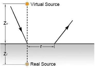
Effective transport coefficient is 𝜎𝑡𝑟 = √3𝜎𝑎𝜎𝑡′. 𝑑𝑟 and 𝑑𝑣 are the distances of the sources from the points at the surface. Thus, by assuming a normal incident light beam shining on the surface of material, we can easily derive:

𝑅_𝑑(𝑟) = 𝑧_𝑟(1 + 𝜎_𝑡𝑟𝑑_𝑟)𝑒−𝜎𝑡𝑟𝑑𝑟

4𝜋𝑑𝑟3 + 𝑧𝑣(1 + 𝜎𝑡𝑟𝑑𝑣)

𝑒−𝜎𝑡𝑟𝑑𝑣

4𝜋𝑑𝑣3 (5)

where 𝑧_𝑟 = 1 𝜎⁄ _𝑡′ and 𝑧_𝑣 = 𝑧_𝑟+ 4𝐴𝐷 are the projected distances in the direction of the normal to the surface while z = 0 represents the surface. Also, the equations

𝑑_𝑟 = √𝑟2_{+ 𝑧}

𝑟2 and 𝑑𝑣 = √𝑟2+ 𝑧𝑣2 represent the distances accurately as the light beam is perpendicular to the surface of the material shown in Figure 1. Also, D = 1 3𝜎_{⁄ 𝑡}′ _{represents the diffusion constant, while A = (1 + 𝐹}

𝑑𝑟)/(1 − 𝐹𝑑𝑟) represents the change in radiance exposure defined in terms of the internal reflection occurring at the surface.

Figure 1. BSSRDF Configuration.

𝛼′ _{is reduced albedo. 𝛼}′_{= 𝜎}

𝑠′⁄𝜎𝑡′. 𝜎𝑠′ and 𝜎𝑡′ are the reduced scattering coefficients affected by the phase function, where 𝜎𝑠′= 𝜎𝑠(1 − 𝑔) , 𝜎𝑡′= 𝜎𝑠′+ 𝜎𝑎 . A =

reflections off the surface. The relative index of refraction 𝜂 of the material is used to calculate 𝐹_𝑑𝑟 using the Fresnel formula:

𝐹_𝑑𝑟 ≈ {−0.44 + 0.71 𝜂⁄ − 0.33 𝜂

2

⁄ + 0.06 𝜂⁄ 3, 𝜂 < 1

− 1.44 𝜂⁄ 2+ 0.71 𝜂⁄ + 0.67 + 0.06𝜂, 𝜂 > 1 (6)

Oblique Incident Angles

The directional dipole diffusion is used to deal with the oblique incidence angle based on the physic, [3]. However, the inclination angle of the incident beam with the diffusion profile can cause a significant near-surface effect, which can be reduced by introducing an empirical correction factor. Donner et al. optimized the light emittance based upon the diffusion approximation [10]. By introducing an attenuation function

κ(x), we can shift the reflectance profile of the beam. By assuming that light scattering is always within the material, we have:

κ(x) = 1 − 𝑒−𝜎𝑡𝑥 ₍₇₎

Figure 2. BSSRDF Configuration with oblique incident light.

The actual sources are the infinite ones along the direction of the refraction (Figure 2); hence, we can use equation 7 to calculate the integral of the spatial differential:

R_𝑟𝑖(r) = ∫ κ(d𝑟)𝑒−𝜎𝑡

′_𝑥

[𝑧_𝑟(1 + 𝜎𝑡𝑟𝑑𝑟)

𝑒−𝜎𝑡𝑟𝑑𝑟

4𝜋𝑑𝑟3 + 𝑧𝑣(1 + 𝜎𝑡𝑟𝑑𝑣)

𝑒−𝜎𝑡𝑟𝑑𝑣 4𝜋𝑑𝑣3 ]𝑑𝑥

∞

0 (8)

where 𝑧_𝑟 = 𝑥 cos 𝜃 and, 𝜃 is the refraction angle between the refracted beam and the normal off the surface.

Approximate Reflectance Profile

Sum of a series of Gaussians provides optimal solutions for the approximation of the reflectance profile. A good-fitting approximate curve describes a sum of two exponential functions proportional to the reciprocal distance which is shown as follows:

𝑅_𝑑 = 𝑒−𝑟 𝑑⁄ +𝑒−𝑟 3𝑑⁄

8𝜋𝑑𝑟 (9)

where d determines the scale of curves described by the Equation 9. Parameter s are set to the reciprocal of d, and the surface albedo A is defined as follows:

A = ∫ Rd(r)2πrdr ∞

which ranges from 0 to 1 because of volume scattering and absorption. Thus, we have:

𝑅_𝑑 = 𝐴𝑠𝑒−𝑠𝑟+𝑒−𝑠𝑟 3⁄

8𝜋𝑟 (11)

OPTIMIZED APPROXIMATE REFLECTANCE PROFILE

Regardless of obliqueness of the incident light, reflectance profile follows the form of dipole model that contains two exponential terms as shown in equation 5. Based on the previous theories in 2.1-2.3, equation 11 can be redefined as follows:

𝑅𝑑 = 𝐴𝑠

𝐵1𝑒−𝑠𝑟+𝐵2𝑒−𝑠𝑟 𝐵3⁄

8𝜋𝑟 (12)

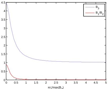
The coefficients before exponential terms, B1 and B2 are determined by the

locations of two sources and transport coefficient. The index of second exponential term, B3, is the ratio of dv to dr.

As the distances from any point to real source and virtual source are different, the coefficients in two exponential terms, B1 and B2, also have different values. The value

of B3 must, be larger than 1 because projected distance from the virtual source to the

surface is larger than projected distance from the real source to the surface. On the other hand, if r is equal to zero than the distance between incoming and outgoing rays is zero at the surface and, B3 will become maximal. Given the relative index of refraction η = 1.3 for whole milk, we can easily calculate the ratio of dv to dr which is 4.44 by

assuming the same point for both incident light and the outgoing ray. In other words, the maximum value of B3 is equal to 4.44 which is a higher result than the one in equation

11.

Figure 3. The relationship between B3, B1/B2 and r respectively for whole milk.

Assuming tanθ = rσ_t′/B3m, where θ is calculated using dr and r and, B3m is the maximum of B3 for any material, then we have

𝐵₃ = √ 𝑡𝑎𝑛2𝜃+1

(𝑡𝑎𝑛2_𝜃+1)/𝐵

3𝑚 (13)

𝐵1

𝐵2=

𝑡𝑎𝑛2_{𝜃+1+(𝑡𝑎𝑛}2_𝜃+1)3_{2√3(1−∝}′₎

(𝐵3𝑚2𝑡𝑎𝑛2𝜃+1) 3

2_{(𝑡𝑎𝑛}2_𝜃+1)−12_{+𝐵3𝑚√3(1−∝}′_)(𝐵

3𝑚2𝑡𝑎𝑛2𝜃+1)√𝑡𝑎𝑛2𝜃+1

(14)

0 0.5 1 1.5 2 2.5 3 3.5 4 4.5 5

0 0.5 1 1.5 2 2.5 3 3.5 4 4.5

r_t,/max(B₃)

The ratio of B₁ to B₂ is computed using equation 14, and the scale of B₁ and B₂ is calculated using energy conservation. The result is shown in Figure 4.

RESULTS

A = 0.20

A = 0.50

A = 0.80

Figure 4. Fit of various reflectance profile models for surface albedos A = 0.2, 0.5, and 0.8.

respectively 0.145, 0.203, 4.2 as seen on the curve in Figure 3. The results show that our approximation is close to the Monte Carlo reference with very small energy loss.

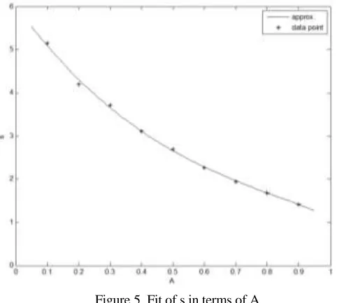
Figure 5. Fit of s in terms of A.

The Figure 5 shows the relationship between A and s. The approximation function is as follows:

s = −3.1229𝐴3+ 8.3943𝐴2 − 10.16𝐴 + 6.0302 (15) The average relative error is approximately 1.02% from the s in the previous simulation. There is not much difference between the shape of the curve and simulated data.

FUTURE WORKS

A new equation is derived from previous studies on subsurface scattering without beam diffusion distribution. Future work would contain the angular term to optimize the reflectance profile near the surface. Also, the different objects may vary in terms of physical properties that result in slight changes to the parameters.

REFERENCES

1. C. Donner, Jason L., Ravi R., Toshiya H., Henrik W., Jensen and Shree N. 2009. “An Empirical BSSRDF Model,” in ACM Transactions on Graphics, 28(3).

2. Ralf Habel, Per H. Christensen and Wojciech J. 2013. “Photon Beam Diffusion: A Hybrid Monte Carlo Method for Subsurface Scattering,” in Computer Graphics Forum (The Eurographics Association and Blackwell Publishing Ltd), 32(4).

3. J. R. Frisvad, Toshiya Hachisuka, and Thomas K. K. 2014. “Directional Dipole Model for Subsurface Scattering,” in ACM Transactions on Graphics.

4. P. Christensen, and B. Burley. 2015. “Approximate Reflectance Profiles for Efficient Subsurface Scattering,” ACM SIGGRAPH, 2015, Talks Article.25.

5. JT Kajiya. 1986. “The Rendering Equation,” in ACM Siggraph Computer Graphics, 20(4):143-150. 6. Jensen, H. W. and Christensen, P. H. 1998. “Efficient simulation of light transport in scenes with

7. Jensen H. W., Marschner S. R., Levoy M., and Hanrahan P. 2001. “A practical model for subsurface light transport,” in Proceedings of ACM SIGGRAPH, 200: 511-518.

8. D’Eon, E., and Irving, G. 2011. “A quantized-diffusion model for rendering translucent materials,” in

ACM Transactions on Graphics (TOG), 30, ACM, pp.56.

9. R. Aronsen, 1995. “Boundary Conditions for Diffusion of light,” Journal of the Optical Society of America An Optics Image Science & Vision, 12(11):2532-2539.

10. C Donner, and HW Jensen. 2007. “Rendering translucent materials using photon diffusion,”