University of Huddersfield Repository
Abdulshahed, Ali, Longstaff, Andrew P., Fletcher, Simon and Myers, Alan
Application of GNNMCI(1, N) to environmental thermal error modelling of CNC machine tools
Original Citation
Abdulshahed, Ali, Longstaff, Andrew P., Fletcher, Simon and Myers, Alan (2013) Application of
GNNMCI(1, N) to environmental thermal error modelling of CNC machine tools. In: The 3rd
International Conference on Advanced Manufacturing Engineering and Technologies. KTH Royal
Institute of Technology, Stockholm, Sweden, pp. 253262. ISBN 9789175018928
This version is available at http://eprints.hud.ac.uk/id/eprint/19044/
The University Repository is a digital collection of the research output of the
University, available on Open Access. Copyright and Moral Rights for the items
on this site are retained by the individual author and/or other copyright owners.
Users may access full items free of charge; copies of full text items generally
can be reproduced, displayed or performed and given to third parties in any
format or medium for personal research or study, educational or notforprofit
purposes without prior permission or charge, provided:
•
The authors, title and full bibliographic details is credited in any copy;
•
A hyperlink and/or URL is included for the original metadata page; and
•
The content is not changed in any way.
For more information, including our policy and submission procedure, please
contact the Repository Team at: [email protected].
Application of GNNMCI(1, N) to environmental thermal
error modelling of CNC machine tools
Ali M Abdulshahed, Andrew P Longstaff, Simon Fletcher, Alan Myers
Centre for Precision Technologies, University of Huddersfield, UK, HD1 3DH
Email: [email protected]
ABSTRACT
Thermal errors are often quoted as being the largest contributor to inaccuracy of CNC machine tools, but they can be effectively reduced using error compensation. Success in obtaining a reliable and robust model depends heavily on the choice of system variables involved as well as the available input-output data pairs and the domain used for training purposes. In this paper, a new prediction model “Grey Neural Network model with Convolution Integral (GNNMCI(1, N))” is proposed, which makes full use of the similarities and complementarity between Grey system models and Artificial Neural Networks (ANNs) to overcome the disadvantage of applying a Grey model and an artificial neural network individually. A Particle Swarm Optimization (PSO) algorithm is also employed to optimize the Grey neural network. The proposed model is able to extract realistic governing laws of the system using only limited data pairs, in order to design the thermal compensation model, thereby reducing the complexity and duration of the testing regime. This makes the proposed method more practical, cost-effective and so more attractive to CNC machine tool manufacturers and especially end-users.
KEYWORDS: Machine tool, Thermal error, Modelling, Grey neural network.
1.
INTRODUCTION
Longstaff et al. [2] presented several Environmental Temperature Variation Error (ETVE) tests conducted on a wide range of machine tools and discussed the implications for produced parts. The authors also described a number of interesting phenomena when the machines were subjected to a wide variety of environmental conditions. Attention was also drawn to the prohibitive downtime required to conduct the ETVE test. Modification of the machine shop conditions is possible and can effectively reduce thermal errors on a number of machines at once, but may be difficult and costly to achieve. Fletcher et al. [4] provided useful information about daily cyclic environmental temperature fluctuations and associated drifts. Experimental results indicated, through error compensation, a reduction of the environmental errors by more than 50% to just ±7μm over a 65 hour test, but also drew attention to the detrimental amount of machine downtime for the thermal characterisation tests. Rakuffand Beaudet [5] measured and modelled the ETVE of a machine tool over 23 h with no traffic in the workshop. They show how certain process variables, such as opening and closing of doors around the machine, affect the ETVE. Mian et al. [6] proposed a novel offline environmental thermal error modelling approach based on a finite element analysis (FEA) model that reduces the machine downtime usually needed for the ETVE test from a fortnight to 12.5 hours. Their modelling approach was tested and validated on a production machine tool over a one-year period and found to be very robust. However, building a numerical model can be a great challenge due to problems of establishing the boundary conditions and accurately obtaining the characteristic of heat transfer.
Research on thermal error compensation for machine tools by both academic institutions and industry has been rapidly accelerated recently in response to the growing demand of product quality. Effective compensation depends on the accuracy of the prediction model. Thermal error modelling and compensation techniques introduced to date have been found to suffer from a number of drawbacks that make their application in practical machining environments time consuming. Different structures of empirical models have been used to predict thermal errors in machine tools such as multiple regression analysis [7], artificial neural networks [7], adaptive neuro-fuzzy inference system [8, 9], Grey system theory [10] and a combination of several different modelling methods [11].
Whilst empirical models can be good at predicting thermal errors, they require a large amount of data with different working conditions to determine the governing laws of the original data. However, a realistic governing law may not exist even when a large amount of data has been measured. Furthermore, the process of obtaining such data can take several hours for internal heating tests and several days or more for the environmental test.
This paper aims to develop an effective and simple method to predict the Environmental Temperature Variation Error (ETVE) of machine tools. The work proposes a novel Grey Neural Network model with Convolution Integral GNNMCI(1,N), combining the Grey prediction model with convolution integral GMC(1,N) and PSO neural network model, and also adopting the GMC(1,N) model when selecting the inputs. The proposed model is a type of dynamic model described by a PSO neural network to extract realistic governing laws of the system using only a limited number of data pairs. The dynamic characteristic of the GNNMCI(1,N) model results from introducing the Grey accumulated generating operation (AGO) into the neural network. The benefits and novelty of this work are that a thermal model can be efficiently built with the minimum amount of temperature data in a very short time scale.
2.
MODELLING THE THERMAL ERROR USING A GREY
The Grey systems theory, established by Deng in 1982 [12], is a methodology that focuses on solving problems involving incomplete information or small samples. The technique works on uncertain systems with partially known information by generating, mining, and extracting useful information from available data. So, system behaviours and their hidden laws of evolution can be accurately described. GM(1, N) is the most widely used implementation in literature [13], which can establish a first-order differential equation featured by comprehensive and dynamic analysis of the relationship between system parameters. The accumulated generating operation (AGO) is the most important characteristic of the Grey system theory, and its benefit is to increase the linear characters and reduce the randomness of the samples. Based on the existing GM(1,N) model, Tzu-Li Ties [14] proposed a GMC(1,N) model, which is an improved grey prediction model. The modelling values by GM(1,n) are corrected by including a convolution integral. However, Grey models lack the ability to self-learn, self-adapt or otherwise considering a feedback value.
Compared with other empirical models, artificial neural networks (ANNs) have a strong capacity for processing information, parallel processing, and self-learning. However, they have some disadvantages such as the need for a large number of learning samples, thus needing a long training computation time, and the non-interpretable problem of such “black box” systems. In addition, the working conditions of machine tools are in general complex and susceptible to unexpected noises. Therefore, ANN models in isolation have significant drawbacks as a modelling approach for thermal error compensation [3].
Because the way of presenting information for neural network and Grey models have some commonality in format, the two methods can be fused. Two levels can be added; an initial Grey level will process the input information and a whitening level after to process the output information to obtain good results [15]. Therefore, the Grey meaning is contained in the neural network. The advantages of both can be used to build a high-performance neural network model with a minimum amount of training data.
2.1. GNNMCI(1, N) Prediction Model
The fusion model of Grey system and neural network is employed in the modelling of the ETVE of machine tools. The model can reveal the long-term trend of data and, by driving the model by the AGO, rather than raw data, can minimize the effect of some of the random occurrences. Therefore, the first step for building GNNMCI(1,N) is to carry out 1-AGO (first-order Accumulated Generating Operation) to the data, so as to increase the linear characteristics and reduce the randomness from the measuring samples. Then the GNNMCI(1,N) model is trained with a PSO algorithm to generate the desired GNNMCI(1,N) model. Finally an IAGO (inverse Accumulated Generating Operation) is performed to predict the ETVE and generate the final compensation values. The model fully takes the advantages of neural networks and Grey models, and overcomes the disadvantages of them, achieving the goal of effective, efficient and accurate modelling. The modelling details are described as follows:
The Grey prediction model with convolution integral GMC(1, n) [14] is:
̂ ∑ { [ ]}
Where is the unit step function [14]; ∑ k=1,2,….,n. To calculate the coefficients bj and , the neural network method can be used to map
equation (2) to a forward neural network. Then, the neural network model is trained until the performance is satisfactory. Finally, the optimal corresponding weights are used as the Grey neural network weights to predict ETVE.
We can process equation (2) more. Let
∑ { [ ]}
We can rewrite equation (2) as:
̂ ( ) (4)
Then equation (4) can be converted into equation (5) as follows:
̂ [
]
̂ [ (
) ]
[
]
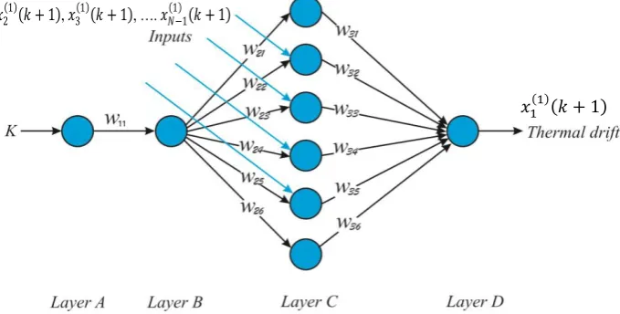
[image:5.479.63.403.435.607.2]Map equation (5) into a neural network, and the mapping structure is shown in Fig. 1.
Fig. 1. The mapping structure of GNNMCI(1, N).
𝑥 𝑘
Where k is the serial number of input parameters;
In this study, is chosen as the thermal displacement data series (network output) and , , …. , as a data seies of temprature sensores (N is the number of network inputs);
are the weights of the network;
Layer A, layer B, layer C, and layer D are the four layers of the network, respectively. Where, the corresponding neural network weights can be assigned as follows:
Let us assume that
The bias value of is:
( ) (6)
The transfer function of Layer B is a sigmoid function
, the transfer functions
of other layer’s neuron are adopted as a linear function
2.2. GNNMCI(1, N) learning algorithm
The learning algorithm of GNNMCI(1, N) can be summarised as follows:
Step 1: For each input series, , the output of each layer is calculated.
Layer A:
Layer B:
Layer C: Layer D:
Step 2: A PSO algorithm [16] is adopted to train the GNNMCI(1, N) model. Each weight of model is encoded to each component of particle position, which means that each particle represents a specific group of weights. In the course of training, the model is repeatedly presented with training pairs. The model parameters are then adjusted until the errors between the predicted output and real output meet a tolerance criterion, or a pre-determined number of epochs has passed (in this work, ten training epochs are determined as the stopping criteria).
Step 3: export the optimal solution. ( ).
3.
EXPERIMENTS
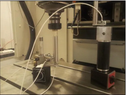
placed around the machine to detect the ambient temperature. Four non-contact displacement transducers (NCDTs) were used to measure the displacement of a test bar (used to represent the tool) while the spindle remained stationary. Three were used to measure displacement of the test bar in each axis direction. A fourth directly monitored displacement of the casting next to the spindle in the Z-axis direction to differentiate expansion of the tool from the machine. A general overview of the experimental setup is shown in Fig. 2.
Fig. 2. A general overview of the experimental setup.
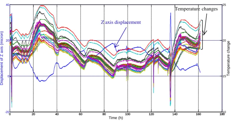
Results of an ETVE test are shown in Fig. 3. This test was carried out over a five-day period during spring bank holiday, with no significant activity in the workshop, followed by approximately three normal working days (160 hours). This data was sampled once every minute. The environmental temperature conditions for machine shop change due to the day /night cycle, where the temperature fluctuates by about 5 ˚C throughout the day, with lower temperatures in the morning and higher temperatures in the late afternoon and evening. The strongest response to the ambient change from the machine is in the Z-axis direction. There is a clear relation between the fluctuation in the environmental temperature and the resulting displacement. For example, the anomaly at the beginning of the test can be attributed to a short period (30 minutes) of the workshop door being opened. Externally, the conditions were snowy, which caused a drop in workshop temperature to below 11˚C. The overall movement caused by this phenomenon is 35 μm in the Z-axis and 25 μm in the Y- axis for an overall temperature swing of approximately 9 ˚C over the 30 minutes. Two similar events can be seen between 120 and 140 minutes. The magnitude of the environmental error can be compared to that from two hours spindle-heating test conducted according to ISO-230:3 which only produced 30µm of error in the Z-axis.
Fig. 3. Temperature measurements and machine movement due to environment.
For this study, a GNNMCI(1, 5) with a structure of 1-1-6-1was chosen. The details are: layer A has one node, the input time series k; layer B has one node; layer C has six nodes, the input variables nodes are from two to five, respectively; T1, T2, T5, and T9 are the input variable data. Layer D has an output variable node, which is the thermal displacement in Z-axis direction. The GNNMCI(1, 5) structure is shown in Fig. 1. The MATLAB software was used to realize the model.
Two compensation methods can be used to predict ETVE. The first is an off-line, pre-calibrated method. This means to obtain the GNNMCI(1, 5) model according to the thermal displacement and the temperature change during a short test, and then to use this model to predict the thermal displacement of other processes. The second method is to obtain the GNNMCI(1, N) model at the first stage of the manufacturing process, and then to use this model to predict the machine movement during the rest of the process. This uses additional measurement effort before the process begins.
To apply the first method, another test was carried out for 80 minutes on the same machine during a normal working day. During the experiment, the thermal errors were measured by the NCDTs and the temperature data was measured using the same selected sensors, sampling every ten seconds. The training samples were obtained from the first 5 readings (less than one minute) after the test had been started. All raw data was converted to AGO series, as discussed in section 2.1. Ten training epochs are adapted as the stopping criteria. In the PSO neural network, the number of population was set to be 90 whilst the maximum and minimum velocity values were 1.5 and -1.5, respectively. These values were obtained by optimization.
After finishing the training of the model, there were two ways to obtain the prediction values: directly obtaining the prediction values from the trained model; or taking out the Grey differential equation parameters from the trained model to equation (2) and then solving the equation to obtain the prediction values. Although both methods are similar theoretically, a large number of experiments have found that the first method needs less computation. Fig. 4 shows simulation results for 80 minutes.
0 20 40 60 80 100 120 140 160 180
-20 0 20 40
D
is
plac
em
ent
of
Z
ax
is
(m
ic
ron)
Time (h)
0 20 40 60 80 100 120 140 160 18010
15 20 25
T
em
perat
ure
c
hang
e
Z axis displacement
Fig. 4: Simulation results for 80 minutes.
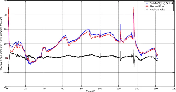
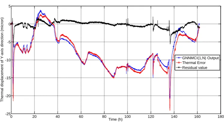
The process was repeated to create a GNNMCI (1, 5) model for the Y-axis direction. To validate the robustness of these proposed models on non-training data, a normal environmental simulation was run using the temperature data presented in Fig. 3. The measured and simulated profile results were plotted for the Z-axis and Y-axis. Compared to the measured results, the correlations were 97% for the Z displacement profiles Fig. 5, and 98% for the Y displacement profiles Fig. 6. The residual errors were less than ± 10 μm for the Z axis and less than ± 6 μm for the Y axis even when considering the rapid changes due to the opened workshop door. Under more predictable conditions, which could be achieved by better management of the environment, ±3µm would be achieved in each axis. Thus, the proposed GNNMCI (1, 5) model can predict the normal daily cyclic error accurately and also can track sudden changes of thermal error from a relatively small training sample.
Fig. 5.Correlation between the measured and simulated Z-axis displacement.
0 10 20 30 40 50 60 70 80
-5 -4 -3 -2 -1 0 1 Time (Minutes) T h e rm a l d isp la ce m e n t (m icr o n ) GNNMCI(1,N) Output Thermal Error Residual value
0 20 40 60 80 100 120 140 160 180
[image:9.479.49.417.414.606.2]Fig. 6. Correlation between the measured and simulated Y-axis displacement.
2.
CONCLUSIONS
Temperature-induced effects on machine tools are a significant part of the error budget. Changes in ambient conditions are an often overlooked effect that can be difficult to model, especially in unpredictable environments.
In this paper, a novel thermal error modelling method based on Grey system theory and neural networks was developed to predict the environmental temperature variation error (ETVE) of a machine tool. The proposed model has been found to be flexible, simple to design and rapid to train.
The model is trained using data obtained from a short test of less than ninety minutes, which is desirable for minimising machine downtime. The accuracy of the model has not been compromised by restricting the training data. ETVE results in the Z-axis direction over a 160 hour test showed a reduction in error from over 20µm to better than ±3µm considering the normal daily cycles. When also considering unexpected phenomena, such as the rapid change in temperature when a workshop door was opened, the model still performs well, with an improvement from 40µm to less than ±10µm.
Similar results were achieved in the Y-axis direction, with this study not considering the X-axis direction due to symmetry of the machine.
It is anticipated that further improvement in correlation could be achieved by including rapid changes as part of the training data. However, this would compromise the aim of this work which is to train the model with “normal” data, but validate across a range of conditions.
The proposed method is a significant advantage over other models based on a single technique that have been used by many previous scholars where the data used to build the models is obtained from very long tests. The proposed model has significantly reduced the machine downtime required for a typical environmental testing from hours to only few minutes. According to experimental work, little machine downtime is needed to apply this modelling approach except to re-establish the model if needed.
The thermal error compensation model using GNNMCI(1, N) introduced in this study can be applied to any CNC machine tool because the model does not rely on a parametric model of the thermal error behaviour. In addition, this method is open to extension of other
0 20 40 60 80 100 120 140 160 180
-25 -20 -15 -10 -5 0 5
Time (h)
T
herm
al
dis
plac
em
ent
of
Y-ax
is
direc
tion
(m
ic
ron)
different physical inputs meaning that alternative sensors can be deployed with minimal retraining required.
ACKNOWLEDGEMENTS
The work carried out in this paper is partially funded by the EU Project (NMP2-SL-2010-260051) “HARCO” (Hierarchical and Adaptive smaRt COmponents for precision production systems application). The authors do wish to thank all the partners of the consortium.
The authors also gratefully acknowledge the UK’s Engineering and Physical Sciences Research Council (EPSRC) funding of the EPSRC Centre for Innovative Manufacturing in Advanced Metrology (Grant Ref: EP/I033424/1).
REFERENCES
[1] J. Mayr, et al., "Thermal issues in machine tools," CIRP Annals - Manufacturing Technology, vol. 61, pp. 771-791, 2012.
[2] A. P. Longstaff, et al., "Practical experience of thermal testing with reference to ISO 230 Part 3," in Laser
metrology and machine performance VI, Southampton, 2003, pp. 473-483.
[3] A. White, et al., "A general purpose thermal error compensation system for CNC machine tools," in Laser
Metrology and Machine Performance V, Southampton, 2001, pp. 3-13.
[4] S. Fletcher, et al., "Flexible modelling and compensation of machine tool thermal errors," in 20th Annual
Meeting of American Society for Precision Engineering, Norfolk, VA, 2005.
[5] S. Rakuff and P. Beaudet, "Thermally induced errors in diamond turning of optical structured surfaces,"
Optical Engineering, vol. 46, pp. 103401-103409, 2007.
[6] N. S. Mian, et al., "Efficient estimation by FEA of machine tool distortion due to environmental temperature perturbations," Precision engineering, vol. 37, pp. 372-379, 2013.
[7] J. Chen, et al., "Thermal error modelling for real-time error compensation," The International Journal of
Advanced Manufacturing Technology, vol. 12, pp. 266-275, 1996.
[8] K. C. Wang, "Thermal error modeling of a machining center using grey system theory and adaptive network-based fuzzy inference system," in Cybernetics and Intelligent Systems, Bangkok, 2006, pp. 1-6. [9] A. Abdulshahed, et al., "Comparative study of ANN and ANFIS prediction models for thermal error
compensation on CNC machine tools," in Laser Metrology and Machine Performance X, Buckinghamshire, 2013, pp. 79-88.
[10] Y. Wang, et al., "Compensation for the thermal error of a multi-axis machining center," Journal of
materials processing technology, vol. 75, pp. 45-53, 1998.
[11] K. C. Wang, "Thermal error modeling of a machining center using grey system theory and HGA-trained neural network," in Cybernetics and Intelligent Systems, Bangkok, 2006, pp. 1-7
[12] D. Ju-Long, "Control problems of grey systems," Systems & Control Letters, vol. 1, pp. 288-294, 1982. [13] L. Sifeng, et al., "A brief introduction to grey systems theory," in Proceeding of IEEE International
Conference on Grey Systems and Intelligent Services 2011, Nanjing, 2011, pp. 1-9.
[14] T.-L. Tien, "A research on the grey prediction model GM (1, n)," Applied Mathematics and Computation,
vol. 218, pp. 4903-4916, 2012.
[15] J. Yuan, et al., "Modeling of Grey Neural Network and Its Applications," in Advances in Computation and Intelligence. vol. 5370, L. Kang, et al., Eds., ed: Springer Berlin Heidelberg, 2008, pp. 297-305.
[16] V. G. Gudise and G. K. Venayagamoorthy, "Comparison of particle swarm optimization and backpropagation as training algorithms for neural networks," in Swarm Intelligence Symposium, 2003.