2018 International Conference on Modeling, Simulation and Analysis (ICMSA 2018) ISBN: 978-1-60595-544-5
Hierarchical Bayesian Estimation of System
Parameters from Dynamic Responses
Qing YANG and Kun ZHANG
*School of Civil and Safety Engineering, Dalian Jiaotong University, Dalian, 116028, China
*Corresponding author
Keywords: Parameter estimation, Uncertainties, Hierarchical Bayesian, Dynamic responses.
Abstract. A hierarchical Bayesian approach is proposed for estimating system parameters by directly taking dynamic responses as the fixed target. The basic theories of hierarchical Bayesian model are first introduced, and then the estimation process of system parameters is illustrated. A mass-spring system of eight degrees of freedom is studied to validate the proposed method, and the effects of modeling errors, incompleteness of dynamic response data and measurement noise on the identification results are numerically investigated. The research results show that the proposed method can accurately identify physical parameters of the system with random modeling errors and measurement noise from only several dynamic responses of the system. This method can provide a new way for parameter estimation of the system with modeling errors, incompleteness of dynamic response data and serous pollution of measurement noise.
Introduction
Parameter estimation from system vibration information and structural model updating, fault diagnosis or damage identification based on the estimated system parameters have been receiving more and more attentions from researchers in the last few decades. However, the nature of the system model and observed data has strong uncertainty under the influence of some factors such as the observation noise, modeling error and environmental factors etc., which causes the estimation of system parameters become a kind of uncertain problems [1].
In this paper, the dynamic responses of systems are directly taken as the fixed target to construct the parameter estimation framework of hierarchical Bayesian model. Firstly, the basic theories of hierarchical Bayesian model are firstly introduced, and the relative estimation process of system parameters from dynamic responses is illustrated. After that, a mass-spring system of eight degrees of freedom is studied to validate the proposed method, and the effects of modeling errors, incompleteness of dynamic response data and measurement noise on the identification results are numerically investigated. Finally, the conclusions of this work are summarized.
Basic Theories of Hierarchical Bayesian Models Based on Dynamic Responses
In the hierarchical Bayesian model based on dynamic responses, the unknown parameters of the system are assumed to obey the Gaussian normal distribution ~N
u,
, and the error function vector is defined as the error between the calculated and the observed dynamic responses from chosen measurements. This can be represented by a multivariate Gaussian distribution as
e e
t D D Nu
e ~~ , (1)
where D and D~ represent the calculated and the observed dynamic responses of the system, respectively. ue is the mean of the error vectors, and e represents the co-variance matrix for the error function.
The posterior probability distribution of the unknown parameters can be expressed as
u t ue e D
P
D t ue e
p
t u
p
u ue e
p ,,
, , ~ ~
, ,
, ,, , (2) Different from the traditional Bayesian method, super parameters are introduced in the prior probability distribution of multistage Bayesian model. u,,ue,e in Eq.(2) all are the over-parameters in this distribution. Before determining the probability distribution, the transcendental probability distribution p
u,,ue,e
of the over-parameters is determined first,and then it constitutes the posterior probability distribution of multistage Bayes together with prior probability distribution and likelihood function.
In the case of having Nt independent data sets, the joint posterior probability distribution function
(PDF) can be stated as
Nt
t
e e t
e e t e
e D P D u p u p u u
u u
p
1
, , , ,
, , ~ ~
, , ,
,
(3)where
t,,
t,
Nt
. It is often reasonable to assume no correlation between these parameters and therefore the co-variance matrix can be presented as a diagonal matrix
2 2 2 2
, , , , ,
2
1 p Np
Diag
, with NP is the number of the unknown parameters in the
vector of . Note that the formulations can be extended for correlated system parameters by estimating all components of the full co-variance matrix . An inverse Gamma probability distribution is assumed for the prior probability of the 2
p
, and that is
2
,1
p
p Inverse Gamma (4) where and can be taken identically for all the unknown structural parameters. Based on the considered priors, the joint posterior probability distribution of all the updating parameters can be stated as
u u D
p t t p t e t N p p N t p tp N t e e t t N p N p N N e u u D J 1 2 1 2 1 1 1 2 2 2 1 2 2 2 2 , , ~ , exp ) ( 1 1 (5) where
e
t e
T e t e e t
t
D
u
e
u
e
u
J
,
~
,
,
1
(6)
p N p p p tp e e t t e e t u u D J D u u p 1 2 2 , , ~ , exp ~ , , , ,
(7)
t N t t t N N N u p t 1 , 1 1 (8)
t N t p tp t p u N ma InverseGam p 1 2 2 2 1 1 , 2
(9)
t e
N t t t N e N N u p t 1 , 1 1 (10)
1 , t N Te e e t e t e t e
t
p InverseWishart
I N e
e
N N
(11)The most common technique to solve Eq. (5) is the Gibbs Sampler, in which samples are generated from the full conditional probability distribution of each parameter until convergence is reached. Convergence is achieved when the changes in statistics of generated samples becomes smaller than a prescribed threshold. After convergence, the MAP estimates of all the updating parameters provide the global maxima of the posterior joint PDF of Eq.(7). The full conditional posterior probability distributions of all the unknown parameters are presented in Eqs.(7)-(11).
It can be observed that the full conditional probability distributions of all the unknown parameters except t are standard distributions.The posterior joint probability distribution of unknown
parameters can be accurately estimated if an adequate number of samples is generated. Generating samples from Eqs. (8)-(11) is trivial due to their known distribution functions. However, when samples are generated from the conditional probability distributions of t by using Eq. (7), it is required to use advanced sampling techniques such as Metropolis-Hasting [6]. Repeat the process until get the smooth Markov chain.The proposed distribution is based on the random distribution of the theoretical values of the unknown parameters in the process.
Numerical Simulation
Model Description
perturbation amplitudes of 5% and 20%, indicating that two levels of measurement noise are contained in the measured data, are simulated to investigate the effect of the observation noise uncertainties on the identification accuracy.
The system is assumed to be excited at the block one (as shown in Fig.1) by a random Gaussian white noise. The sampling frequency and the sampling time of structural dynamic responses are 500 Hz and 1 s, respectively. The identification accuracy is represented by the relative error between the identified stiffness coefficients and the true ones as
% 100
e
j tr
e j tr e j id
j
k k k
e , j=1,2,…,7 (12)
[image:4.595.140.463.248.306.2]where idkej and trkej are the jth identified and true stiffness coefficients respectively.
Figure 1. The schematic of the eight degrees of freedom mass-spring system. Result Analysis
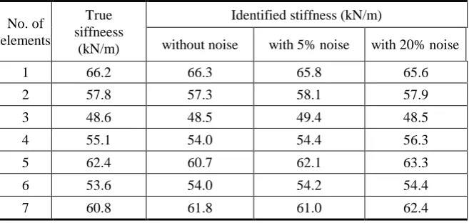
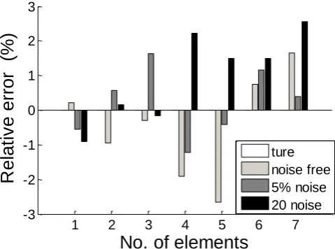
[image:4.595.134.463.514.670.2]Table 1 listed the true random stiffness coefficients of the system and their identified values with different level of noise. Fig.2 illustrates the relative errors between the identified stiffness coefficients and the true ones in the three cases listed in Table 1. As shown in Table 1 and Fig.2, for all the three cases with or without measurement noise, the identified stiffness coefficients all are close to their true values and the absolute maximum relative errors of all the three cases are below 3%. These results indicate the proposed method can accurately identify physical parameters of the system with random modeling uncertainties from only several dynamic responses of the system. The identification errors are mainly caused by the random nature of the Bayesian models, while the uncertainty of measurement noise has little negative influence on the estimating accuracy. The proposed hierarchical Bayesian approach has good robustness to measurement noise.
Table 1. Identification results of the system stiffness coefficients with different level of noise.
No. of elements
True siffneess
(kN/m)
Identified stiffness (kN/m)
without noise with 5% noise with 20% noise
1 66.2 66.3 65.8 65.6
2 57.8 57.3 58.1 57.9
3 48.6 48.5 49.4 48.5
4 55.1 54.0 54.4 56.3
5 62.4 60.7 62.1 63.3
6 53.6 54.0 54.2 54.4
1 2 3 4 5 6 7 -3
-2 -1 0 1 2 3
No. of elements
R
elat
iv
e
error
(%)
[image:5.595.174.414.74.252.2]ture noise free 5% noise 20 noise
Figure 2. The relative errors between the identified stiffness coefficients and the true ones.
Summary
Based on the existing hierarchical Bayesian algorithm, this paper proposes a hierarchical Bayesian system parameter estimation approach from the dynamic responses of the system in time domain. The validity of the proposed method is numerically verified by an eight-degree-of-freedom mass-spring system. The research results show that the proposed method can accurately identify physical parameters of the system with random modeling errors from only several dynamic responses of the system, and has good robustness to measurement noise uncertainty. This method can provide a new way for parameter estimation of the system with modeling errors, incompleteness of dynamic response data and serous pollution of measurement noise. Of course, further investigation on the performance and the validity of approach on identifying experimental or real engineering system are still on the way.
Acknowledgement
This research was financially supported by China National Science Foundation (51108130), Science Foundation of Liaoning Province (20170540130), Research Foundation from the Education Department of Liaoning Province (L2014192), and Scientific Research Foundation for Introduced Talents of Dalian Jiaotong University.
References
[1] I. Lopez, N. Sarigul-Klijn, A review of uncertainty in flight vehicle structural damage monitoring, diagnosis and control: Challenges and opportunities, Prog. Aerosp. Sci. 46 (2010) 247-273.
[2] J. L. Beck, L.S. Katafygiotis, Updating models and their uncertainties I: Bayesian statistical framework, J. Eng. Mech-ASCE 124 (1998) 455-461.
[3] M. W. Vanik, J. L. Beck, S.K. Au, Bayesian probabilistic approach to structural health monitoring, J. Eng. Mech-ASCE 126(2000) 738-745.
[4] J. L. Beck, S. K. Au, Bayesian Updating of Structural Models and Reliability using Markov Chain Monte Carlo Simulation, J. Eng. Mech-ASCE 128(2002) 380-391.
[5] W. J. Yan, L.S. Katafygiotis, A novel Bayesian approach for structural model updating utilizing statistical modal information from multiple setups, Struct. Saf. 52(2014) 260-271.
[7] E. P. Carden, Vibration based condition monitoring: A Review, Struct. Health Monit. 3(2004), 355-377.
[8] C.R. Farrar, D.A. Jauregui, Comparative study of damage identification algorithms applied to a bridge: I. Experiment, Smart Mater. Struct. Vol. 7(1998) 704-719.