MEMS microstructured surface characterisation based on wavelet transform techniques

Zhu, Hao, Xiao, Shaojun, Jiang, Xiang and Blunt, Liam

MEMS microstructured surface characterisation based on wavelet transform techniques

Original Citation

Zhu, Hao, Xiao, Shaojun, Jiang, Xiang and Blunt, Liam (2008) MEMS microstructured surface 

characterisation based on wavelet transform techniques. In: Proceedings of Computing and 

Engineering Annual Researchers' Conference 2008: CEARC’08. University of Huddersfield, 

Huddersfield, pp. 87­92. ISBN 978­1­86218­067­3 

This version is available at http://eprints.hud.ac.uk/id/eprint/3685/

The University Repository is a digital collection of the research output of the

University, available on Open Access. Copyright and Moral Rights for the items

on this site are retained by the individual author and/or other copyright owners.

Users may access full items free of charge; copies of full text items generally

can be reproduced, displayed or performed and given to third parties in any

format or medium for personal research or study, educational or not­for­profit

purposes without prior permission or charge, provided:

•

The authors, title and full bibliographic details is credited in any copy;

•

A hyperlink and/or URL is included for the original metadata page; and

•

The content is not changed in any way.

For more information, including our policy and submission procedure, please

contact the Repository Team at: [email protected].

STABILISING FIBRE INTERFEROMETERS

H. Martin and X. Jiang

University of Huddersfield, Queensgate, Huddersfield HD1 3DH, UK

ABSTRACT

Fibre interferometry holds many advantages for the online measurement of high precision surfaces. However, the method requires stabilising against path length change due to temperature drift and vibration. A method of stabilising such an interferometer using intensity feedback was examined and shown to be ineffective at low frequencies. A second method, using real-time calculated phase feedback was also investigated, and was observed to be more robust.

Keywords fibre interferometer vibration stabilised

1. INTRODUCTION

Technological advances in several fields have resulted in the increased use of nano-scale and ultra-precision surfaces. Such fields include optics, hard disc manufacture, micro-moulding and micro machining. Multi-axis machining and micro-fabrication techniques are seeing surfaces with sub-micron form accuracy and the production of nano-scale surface features. With ever decreasing manufacturing scales the current state of online metrology methods is found to be severely lacking.

Optical interferometric techniques for metrology hold many advantages such a speed, resolution, traceability and ncontact measurement. They are not however very suitable for application to on-line measurement due to the fact that any height disturbance is mapped directly onto the measurement result. This research hopes to try and alleviate this issue by providing immunity to disturbance during the measurement interval by way of active vibration compensation, thus realising an instrument with the benefits of an optical interferometer, but which is suitable for on-line applications.

In surface measurement applications, interferometers may be used to determine surface height variation by a variety of methods. They all have one element in common however, the determination of the phase value of the interferogram resulting from two interfering wave fronts. One wave front is a known reference, and the other is retro-reflected from the measurand. The resulting phase map, along with knowledge of the illuminating wavelength reveals a representation of the surface topology.

Interferometers are well established for high precision surface measurement, but they are in general full-field bulk optics devices in which a whole area is imaged and captured. Such devices are large and heavy and as such, unsuitable to on-line surface measurement. Another approach is to use single-point scanning, the idea being analogous to a traditional contact stylus, but realised in the optical domain. The concept of an optical stylus provides the advantages of speed and non-contact measurement.

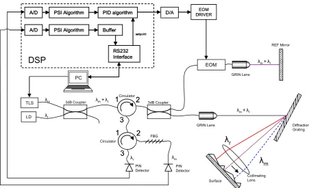
The optical stylus technique can be combined with optical fibre to produce a compact probe which is more suitable for use on-line. Not only is such a probe small and compact, but the requirements for alignment may be relaxed for a single point system. By using optical fibre, the probe can be mounted remotely from the interrogation apparatus. Single point scanning may be enabled by using a swept wavelength source, and a diffraction grating within the probe to create angular dispersion. In this way the optical stylus may be scanned along one axis, thus determining a height profile. The experimental set up investigated in this paper is shown in figure 1. Optical fibre interferometers, whilst providing a novel solution for some surface measurement applications, come with their own set of challenges however; these must be overcome to realise their full potential.

modulation in fringe visibility, and if any of the optical components show any polarisation dependence, variance in intensity. Mitigating the effects of these disturbances is essential if we are to gauge any meaningful information from the phase data acquired from a fibre interferometer. Optical path length change imposes itself directly on the measurement result, distorting the data. The magnitude of the path length change scales with the length of fibre; with approximately 20 metres of fibre in the current experimental setup, temperature drift alone can result in several microns of path change, completely obliterating any measurement at the nanometric scale.

2. INTENSITY FEEDBACK

By multiplexing two interferometers using separate source wavelengths, one may be used as a reference interferometer to track the path changes occurring due to environmental disturbance. If a suitable actuator is present in the system, the output from this interferometer can then be used as feedback in a closed loop to stabilise the interferometer. Because the reference interferometer beam remains stationary on the measurand surface during the measurement interval, the closed loop system can also attenuate the effects of vibration on the surface itself. This provides the possibility of making nanometric resolution measurements in unstable environments, a major boon to any online measurement methodology.

Previous work has shown that using a mirror mounted on a piezo-electric translator (PZT) and placed in the reference arm to modulate path length works well, but has a limited frequency response due to the dynamic limits of the PZT (Martin et al., 2008). This work replaces the PZT with an electro-optic phase modulator (EOM) in order to alter the path length. The main advantage of this technique is the hugely increased frequency response which extends to 1 GHz with the device used (Eospace). With such a device implemented, it is actually the response of the photo-detectors and their associated transimpedance amplifiers that produce the upper limit. EOMs take advantage of the Pockels effect, present to a relatively large degree in certain crystal types (in this case Lithium Niobate). By applying an electric field across the active crystal axis, the refractive index may be altered over that region; in this way the optical path length is also changed. Whilst there are clear advantages in using EOMs for their high frequency response, linearity and lack of moving parts, they invite some complications to proceedings.

In order to prove the concept of using an EOM in place of a PZT to stabilise an interferometer in the face of environmental disturbance, a proportional-integral (PI) controller was designed using high speed op amps. This was then used to actuate the EOM, feedback being obtained from the interferometer by way of PIN photodiodes. As with any control system, in order to provide robust and responsive control, suitable control parameters must first be chosen. The intensity response,

I

of an interferometer is given by;

[

cos

(

t

)

]

I

I

I

I

I

=

r

+

m

+

r m

⋅

ϕ

(1)

Where

I

r,

I

m are the light intensities from the reference and measurement arms respectively.

ϕ

(

t

)

is

the disturbance induced time varying phase difference between the two arms.

Modelling such a system is difficult, the dynamics of an interferometer are non-linear, due to the cosinusoidal response apparent from (1) and the associated modulo 2π ambiguity. Clearly the process parameters are position dependant, but if we assume the interferometer is to be held at quadrature, we can approximate a linear response over a small range of excursion. With this simplification in mind it is possible make use of the First Order Plus Dead Time (FOPDT) model to represent the response. The s-domain representation in transfer function format is;

p s p

sT

e

K

s

U

s

Y

p

+

⋅

=

−

1

)

(

)

(

θ

(2)

Where

Y

(

s

)

,

U

(

s

)

,

K

p,

T

_p and

θ

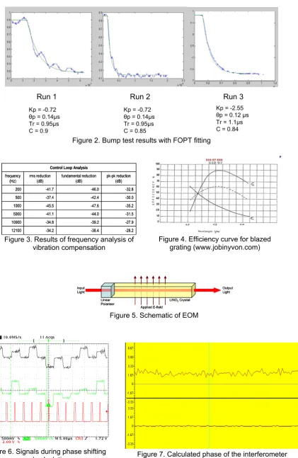
p are the process response, input, gain, time constant and dead

traces show the process (interferometer) response while green is the fitted FOPDT model. The first two runs were done with the same interferometer setup; the third was performed after having optimised the interferometer for maximum visibility. The magnitude of the step was such that it moved the response over the full range of one fringe. The only parameter that changes with visibility is the process gain, . Although the time constant shows slight variation, this can be accounted for by the ‘fitting by eye’ procedure; the values are within the 20% tolerance of any electronic components will be used to implement a controller anyway.

p

K

With an approximate model determined, internal model control (IMC) rules were used to determine suitable control parameters (Rivera et al., 1986). For a FOPDT model, a PI controller (in the ideal configuration) with IMC determined parameters is given by;

)

(

_{p c}

p p c

T

K

T

K

+

=

θ

and

T

i

=

T

p (3)

Where

K

c is the controller gain,

T

i the integrator reset time and

T

c the controller time constant and

which specifies the controller performance. The value of controller time constant, which creates control response from ‘aggressive’ to ‘conservative’ as defined by the IMC rules, is in the range of

. The final controller type (ideal PI configuration) then takes the s-domain form:

c p

T

T

1

.

0

<

<

10

T

_p

⎟⎟

⎠

⎞

⎜⎜

⎝

⎛

+

⋅

=

i c

sT

K

s

E

s

U

(

)

(

)

1

1

(4)

Where

E

(

s

)

is the error signal input to the controller.

The reference arm of the interferometer was disturbed over one full fringe (equating to 750nm pk-pk disturbance) to test the ability of the control loop to attenuate disturbance. This was done by applying a sinusoidal voltage to a PZT mounted mirror at varying frequencies. The experimental results only go up to 12 kHz as the limit of PZT operation is reached at that point. The quality of reduction does not appear to drop substantially however, so we can infer that the effective frequency response goes much higher. The best figure of merit for measuring the quality of the vibration reduction is not completely obvious. Three separate measurements were therefore taken; the reduction of the RMS value of the signal, the reduction of the fundamental peak and the reduction of the peak-to-peak values. The results are summarised in the figure 3.

The results of the initial test look very promising, with the interferometer locked to a specific voltage. However, when determining the phase of the interferometer over a longer time it appeared that drifting in the measurement was still apparent, even though the output voltage of the reference interferometer remained at the setpoint. In order to explain this we must consider the aforementioned variations in polarisation state within optical fibre.

Generally, the change in polarisation state in fibre may be modelled by considering any length of fibre as a lumped circular birefringence. The axis of orientation and rotational magnitude of the lumped birefringence varies as the core is subjected to stresses and distortions resulting from environmental influences. The result is a constantly evolving state of polarisation (SOP) at any point along a length of fibre (Kersey et al., 1990). SOP variations have two primary effects on the output of an interferometer. First, the fringe visibility,

V

is dependant on;

)

2

/

cos(

φ

=

V

₍₅₎

Where

φ

is the angle between the unit vectors of the SOPs of the two interfering waves when mapped on the Poincaré sphere. Clearly, as the SOPs of the beams meeting at the 3dB coupler vary over time, the fringe visibility varies also.

The efficiency of all diffraction gratings shows some polarisation dependency; generally the p-plane efficiency (parallel to the rulings) decays monotonically while the s-plane characteristic depends greatly on the blaze angle. For the model of grating used in our experiment (Jobin-Yvon 5210-97-020) the blaze angle is 42° 27′, and produces 62% difference in grating efficiency between the s and p plane polarisations at 1550 nm illumination (the curve is shown in figure 4). In our system the light in the measurement arm is diffracted twice on the round trip to the surface, further increasing the effect. Clearly for the randomly varying SOP of the light exiting the fibre, a variation in intensity will be produced back at the coupler; the effect can be described as intensity flickering.

In the reference arm another source of SOP dependant intensity flickering occurs due to the EOM. The schematic of the EOM shown in figure 5 reveals a linear polariser in line with the active crystal axis. This is required to ensure that only the purely phase modulated light is passed; otherwise the EOM would act as a linear birefringence with adjustable phase delay. While providing an important function, the nature of a linear polariser creates intensity flickering as the SOP of the light in the measurement arm changes.

The intensity of the light in each of the two interferometer arms can now be seen as time varying, and coupled with the overall fringe visibility dependence described by (5), we can write a new version of (1);

[

cos

(

)

]

)

(

)

(

)

(

)

(

)

(

t

I

t

V

t

I

t

I

t

t

I

I

=

_r

+

_m

+

_r

⋅

_m

⋅

ϕ

(6)

It should be clear from (6) that the output intensity is not just a function of phase; therefore it is not sufficient to lock the interferometer to a certain intensity value in order to keep it stable. Another method of locking the interferometer more effectively is required.

3. PHASE FEEDBACK

An alternative approach to providing feedback is to lock the interferometer using calculated phase information. This method is resource expensive because of the computational overhead required to provide the feedback signal. The method employed was to use a digital signal processor (DSP) (Texas Instruments TMS320F2812) in order to calculate the phase values on the fly. This was done by shifting the phase of the interferometer stepwise and then sampling the resulting intensity values. The Carré phase shifting algorithm was then executed on the DSP to retrieve the actual phase value (Creath, 1988). The principle concept is that the phase shifting routine should execute much faster than the relatively slowly time varying SOP evolution in the interferometer, making any errors between individual phase shifted intensity values negligible.

The calculated phase values ranging over ±π are then inverted and used as the error signal to a DSP implemented PI controller. The controller then acts on the EOM output in order to keep the calculated phase value at 0 radians. Overall execution time for the phase calculation and control algorithm is approximately 40 μs, yielding an overall control loop rate of 25 kHz. Figure 6 shows various signals occurring during the routines execution. The upper trace is the intensity output of the interferometer and clearly shows the phase stepping occurring due to the voltage applied to the EOM (middle trace). The lower trace (active high) shows the intervals at which the DSP is executing the required storage, phase calculation or control algorithms. It can be seen that the DSP actually spends a substantial amount of time in an idle state; this delay is a combination of the write time and settling time for the digital-to analogue converter (DAC). Currently, the DAC used (AD766JN) is written using a high speed serial link (12 Mbps, SPI interface) and requires 1.5 μs settling time. In the future, the loop rate will be increased by using a parallel loading DAC with a faster settling time, thus reducing the wait time between phase shifts.

Initial results look very promising with the reference interferometer phase output being held steady over a long duration. Modulating the input polarisation of the source had no effect on the output phase stability; however a full study of the vibration compensating ability has yet to be carried out. Calculated phase output for the reference interferometer is shown with the control loop dormant and activated in figure 7, upper and lower traces respectively.

4. CONCLUSION

been shown that this method is not very effective at low frequencies due to the time varying polarisation state evolution within the fibre. Fringe visibility and the light intensities in each interferometer arm are both seen unstable making intensity locking perform poorly. A second method of using rapidly calculated phase values to provide the feedback for a control loop was also investigated. Early results show a much more robust and stable result. Further improvements to the code and electronics should result in an increase in the control loop rate and an improvement in the overall performance.

REFERENCES

Jackson, D.A et al., “Elimination of drift in a single-mode optical fiber interferometer using a piezoelectrically stretched coiled fiber,” Appl. Opt. 19(17), 2926-2929 (1980)

Martin, H. et al., “Vibration compensating beam scanning interferometer for surface measurement,” Appl. Opt. 47(7), 888-892 (2008)

Rivera, D. et al., “Internal Model Control. 4. PID Controller Design,“ Ind. Eng. Chem. Process Des. Dev. 25, 252-265 (1986)

Kersey, A. et al., “Analysis of Input-Polarization-Induced Phase Noise in Interferometric Fiber-optic Sensors and Its Reduction using Polarization Scrambling”, J. Lightwave Technol. 8(6), 838-845(1990). Creath, K., "Phase-Measurement Interferometry Techniques," in Progress in Optics. XXVI, E. Wolf, ed.

(Elsevier Science Publishers, Amsterdam,1988), pp.349-393.

1 2

3

1 2

3

TLS

LD

EOM DRIVER A/D

A/D PSI Algorithm

PSI Algorithm PID algorithm

Buffer

RS232 Interface

setpoint

D/A

PC

EOM DRIVER A/D

A/D PSI Algorithm

PSI Algorithm PID algorithm

Buffer

RS232 Interface

setpoint A/D

A/D PSI Algorithm

PSI Algorithm PID algorithm

Buffer

RS232 Interface

setpoint

D/A

PC PC

1 2

3

1 2

3

λ

_r

λ

_m

REF Mirror

Diffraction Grating

Collimating Lens Surface

PIN Detector

PIN Detector Circulator

Circulator

FBG 3dB Coupler

λ_m λ_r

λ_r

λm λm +λr

λm +λr λm +λr

DSP

3dB Coupler

EOM

GRIN Lens

[image:6.595.86.538.383.658.2]

GRIN Lens

Kp = -0.72

θp = 0.14μs Tr = 0.95μs C = 0.9

Kp = -0.72

θp = 0.14μs Tr = 0.95μs C = 0.85

Run 1 Run 2 Run 3

Kp = -2.55

[image:7.595.83.505.76.724.2]

θp = 0.12 μs Tr = 1.1μs C = 0.84

Figure 2. Bump test results with FOPT fitting

Figure 4. Efficiency curve for blazed grating (www.jobinyvon.com) -28.2 -38.4 -34.2 12100 -27.9 -39.2 -34.8 10000 -31.5 -44.0 -41.1 5000 -35.2 -47.6 -45.5 1000 -30.0 -42.4 -37.4 500 -32.8 -46.0 -41.7 200 pk-pk reduction (dB) fundamental reduction (dB) rms reduction (dB) frequency (Hz)

Control Loop Analysis

-28.2 -38.4 -34.2 12100 -27.9 -39.2 -34.8 10000 -31.5 -44.0 -41.1 5000 -35.2 -47.6 -45.5 1000 -30.0 -42.4 -37.4 500 -32.8 -46.0 -41.7 200 pk-pk reduction (dB) fundamental reduction (dB) rms reduction (dB) frequency (Hz)

Control Loop Analysis

Figure 3. Results of frequency analysis of vibration compensation

LiNO3Crystal

Applied E-field Linear Polariser Output Light Input Light

LiNO3Crystal

Applied E-field Linear Polariser Output Light Input Light

Figure 5. Schematic of EOM

Figure 6. Signals during phase shifting

[image:7.595.90.478.85.265.2]