An analysis of costs in institutions of higher education in England

AN ANALYSIS OF COSTS IN INSTITUTIONS OF HIGHER EDUCATION IN

ENGLAND

Geraint Johnes1

Jill Johnes1

Emmanuel Thanassoulis2

This version: September 2007

1. Lancaster University Management School, Lancaster LA1 4YX, UK 2. Aston Business School, Aston University, Birmingham B4 7ET, UK

ABSTRACT

Cost functions are estimated, using random effects and stochastic frontier methods, for English higher education institutions. The paper advances on existing literature by employing finer disaggregation by subject, institution type, and location, and by introducing consideration of quality effects. Estimates are provided of average incremental costs attached to each output type, and of returns to scale and scope. Implications for the policy of expansion of higher education are discussed.

1. Introduction

During the last three decades, the UK higher education sector has been under pressure to provide its services as efficiently as possible, whilst undergoing huge changes in its size and structure. In 1992, former polytechnics were granted the status of universities. Since then, in the period from 1996 to 2003, total student numbers in the UK higher education sector have increased by 33.5% (with a declared aim of further increasing this so that the age-participation ratio reaches 50% by 2010), income from research grants and contracts has increased by 67.1% and expenditure has grown by 45.7%. Despite the drive for efficiency, little detailed information is available about the structure of costs in the UK higher education sector, yet, in an environment of expanding output and increasing costs, the importance of such a knowledge can surely not be overstated.

Any efficient expansion of output requires a knowledge of marginal cost, average cost, and economies of scale and scope. Higher education institutions (HEIs) are multi-product firms which, in the literature to date, have been assumed to produce two main outputs, namely

teaching and research (Cohn & Cooper 2004). These outputs are themselves composed of outputs that can be defined at a finer level of disaggregation, and which are arguably

heterogeneous – for example, teaching activity can be disaggregated by level and subject. An additional output that has become increasingly important in recent years is often referred to as third mission or third leg output; this encompasses, inter alia, the provision of advice and other services to business, the storage and preservation of knowledge, and the provision of a source of independent comment on public issues (Verry & Layard 1975). The term ‘third leg’ describes the third mission of higher education institutions in the contemporary era – the first two missions, or ‘legs’, are of course teaching and research. The third mission has become increasingly important to institutions following the Lambert Review, which concluded that universities could do much to support the business sector, especially small and medium enterprises. In the wake of this, institutions have internalised much work, on the cusp of

research and consultancy, that previously might have been done by academics in their own time.

The purpose of this paper is therefore to resolve these issues in order to estimate an up to date cost function of the English higher education sector. (We focus on England in order to avoid complications that arise from spatial differences in the higher education system arising from devolution of powers to Scotland and Wales.) Such a function can then be used to establish whether there are economies of scale or scope in English higher education institutions, in an effort to identify the best way of achieving expansion in the sector. In addition, the effect on costs of institution type, location and quality - areas of research which have been largely ignored in earlier analyses of costs - will also be examined in the subsequent analysis.

The paper is in 5 sections of which this is the first. Section 2 considers the methodological issues, and a short review of the literature on costs in UK higher education is provided in section 3. An empirical analysis of costs in more than 120 HEIs in England over a 3 year period is presented in section 4 and conclusions are drawn in section 5.

2. Methodology

Before proceeding to conduct an empirical analysis, there are three methodological questions to address: (i) what is an appropriate functional form for the cost equation? (ii) how can economies of scale and of scope be quantified in a multi-product context? and (iii) what is the appropriate estimating technique to use?

2.1 Functional Form

A cost function is an equation that allows costs (C) to be evaluated, given information about the level of output being produced by an organisation and information about the price (or quality) of the organisation’s inputs. This is written for HEI k as:

(

)

k f y w

C = ,

where y_ik= output i of HEI k (i = 1,…n; k = 1, … ,K) and

w

used in HEI k.

The first cost functions estimated for UK higher education were simple linear functions (Verry & Layard 1975), but these were restrictive and were limited in their ability to model economies of scale with any sophistication. A linear cost function is also unable to model economies of scope (or synergies) that are due to joint production. Thus, in order to perform a satisfactory analysis, more sophisticated cost functions need to be hypothesised. Baumol et al. (1982) have identified three candidate functions which have a number of desirable properties. Of these, we choose the quadratic cost function

( )

_∑∑

∑

+ =

i j

k jk ik ij i

ik i

k a b y c y y v

C 0 1/2

where yik and vk respectively denote type i outputs in the kth institution and an

estimates of cost functions in higher education, this specification does not explicitly include information about factor prices. Most estimates of cost functions in higher education do not include such information. With the exception of London (where a weighting attaches to pay), academics below the rank of full professor in the UK are remunerated on a common pay scale; while this is no doubt applied differently in different institutions, reliable information on factor price differences would be difficult to obtain. Nevertheless, later in the paper we do consider a variation of the model that allows factor prices to vary across groups of institutions based on locale.

2.2 Economies of Scale and Scope

Returns to scale in the context of a single product organisation are a familiar concept, and are often measured by the ratio of average cost to marginal cost; if this ratio exceeds unity, then average cost must be falling and scale economies are being realised. Analogous concepts have been developed for the case of the multi-product institution (Baumol et al., 1982). These concepts include measures of ray economies to scale and product-specific returns to scale (where values above unity indicate that scale economies are unexhausted), and of returns to scope (where values above zero indicate that economies of scope are unexhausted). These concepts are defined in detail in the appendix.

2.3 Estimation Methodology

The final methodological issue which must be addressed concerns the means of estimation. In the present case we have observations on k HEIs over t time periods (that is a panel of data), and so a technique appropriate for estimation in the context of panel data should be employed. The main focus of modelling panel data is how to model the heterogeneity across observations (here, HEIs).

The simplest solution is to adopt a fixed effects approach which allows the unobserved individual effects to be correlated with the included explanatory variables. One problem with this is that the model can only apply to observations in the sample for which the intercept has been estimated. Another difficulty, particularly relevant in the case of the present dataset, is that where the time dimension of the panel is short, most of the variation in the dependent and independent variables is across observations; introduction of fixed effects can then introduce severe multicollinearity and diminish the precision of the coefficient estimates. This difficulty could, of course be addressed by using a longer panel. There is, however, a trade-off between the length of a panel and the confidence we can have in the stability of the estimated parameters over time. The market environment for higher education in England has been fast moving, and so we have chosen to work with a short panel.

distributed over all units, that is a random effects (RE) approach (Scheffe, 1956; Wallace and Hussein, 1969; Nerlove, 1971). The advantage of this is that the number of parameters to be estimated is considerably less than for a fixed effects model. However, if the initial assumption is inappropriate, then estimates may be inconsistent. For HEI k in time period t the model is represented by

kt k kt

kt y u

C = ' β +(α + )+ε

where: kt

C is the observation of the dependent variable for the kth HEI in the tth time period; kt

y is the matrix of n explanatory variables (not including a constant);

α is the intercept term and denotes the mean of the unobserved heterogeneity;

uk is independent and identically distributed with zero mean and variance of σ2α. This should be

interpreted as the random heterogeneity specific to the kth observation and is constant over time; (The assumption of constancy over time can be relaxed at the expense of setting uk a

pre-specified function of time, a refinement we have not pursued in this paper.)

εkt is independent and identically distributed with zero mean and variance of σ2ε; it is

uncorrelated over time.

By assumption, u_k and ε_ktare mutually independent and are independent of x_kt ∀k,t, and so the OLS estimators for α and β are unbiased and consistent. However, since the composite error term u_k +ε_kt exhibits a pattern of autocorrelation (unless σ_α2 =0), generalized least squares (GLS) is used to estimate the RE model.

3. Literature review

Numerous studies of the costs of higher education have been conducted in a variety of countries. In this section, we focus primarily on those that have concerned the UK. The first reported study is an exception, and is included because it is the earliest study of university costs that is based on modern understanding of multi-product organisations (Cohn et al., 1989). These authors use a flexible fixed quadratic function and a cross section of 1887 HEIs to relate total education transfers and expenditures in 1981-82 to three outputs: FTE undergraduate enrolment; FTE postgraduate enrolment; and grants received by the HEI for research. The problem of the possibility of different objectives across HEIs is addressed by splitting the sample into public and private institutions, and performing the analysis separately for each subsample. Cohn et al. generalise the quadratic equation by augmenting it with average faculty salary and its square – something that we do not, owing to data constraints, do in the present paper (though we do experiment with a variable capturing an institution’s location in London, something which we expect to be positively correlated with staffing costs). It is worth noting that Cohn et al. find the salary terms to be statistically insignificant.

The results indicate that there are ray economies of scale up to the mean output level in the public sector and up to 6 times the mean output level in the private sector. Product-specific economies of scale, however, are observed only in the public sector, and only for postgraduate teaching and research output (although economies are also observed in undergraduate teaching in HEIs producing low levels of output). Economies of scope are found in both the public and the private sectors of higher education.

Several studies of costs in the UK higher education sector have also employed a quadratic functional form for the cost function (Johnes 1996; 1998). These studies differ from the Cohn et al. (1989) study, however, because each of the outputs (undergraduate student load, postgraduate student load, and value of research grants) is split by broad subject category, namely arts and science. In addition, the latter of the studies, which are based on data for 50 UK universities in the years 1989-90 and 1990-91, uses SFA as well as least squares to estimate the cost function. Ray economies of scale and product-specific economies of scale for science postgraduate teaching and for science research output are found using both estimating methods. Global economies of scope are observed when least squares is used but not when SFA is used to estimate the quadratic cost function. This reinforces the importance of eliminating inefficiency before addressing the issue of economies of scope or scale.

because the former CATs exploit economies of scale in science but not in arts. Turning to postgraduate teaching, the AIC of science postgraduate teaching exceeds that for science undergraduate teaching in small universities, but the two are virtually identical for a typical university with average levels of output. In the case of arts, postgraduate teaching has a lower AIC than undergraduate teaching in the typical university.

A constant elasticity of substitution (CES) functional form has been used in a number of studies of UK higher education (Johnes 1997; 1999; Izadi et al 2002). All three of these studies use data for 1994/95 (thereby including both pre- and post-1992 universities in the cost function for the first time), and disaggregate only undergraduate students into arts and science categories. The later two studies (Johnes 1999; Izadi et al 2002) differ from the first as they estimate a frontier cost function using SFA. AICs of postgraduate teaching are found to exceed those for undergraduate teaching, and AICs of science undergraduate teaching exceed those of arts undergraduate teaching. Ray economies of scale are close to unity but product-specific economies of scale are observed for arts undergraduate teaching, postgraduate teaching and research. There are no economies of scale for science undergraduate teaching. Economies of scope are observed nowhere.

The translog functional form has been used in several studies of the UK higher education sector (Glass et al 1995a; 1995b; Stevens 2005). The early studies use data for periods when the binary divide between universities and polytechnics was still in existence, and do not disaggregate the three main outputs by subject. These studies confirm the existence of ray economies of scale, and product-specific economies are consistently observed for undergraduate teaching (Glass et al 1995a; 1995b). There is no evidence of global economies of scope, and product-specific economies of scope are observed only for postgraduate teaching, while diseconomies of scope are identified in undergraduate teaching (Glass et al 1995a).

More recent data (academic years 1995/96, 1996/97, 1997/98 and 1998/99) form the basis of analysis in the Stevens (2005) study, which differs further from the Glass et al. (1995a; 1995b) studies because SFA is used to estimate the translog cost function. The only output to be disaggregated by subject is undergraduate teaching. This study is particularly remarkable for its attempt to control for quality by the inclusion of two variables namely A level/Scottish Highers score of the entry cohort, and the percentage of first and upper second class degrees achieved. Interpretation of the results regarding these variables is difficult because of the multicollinearity between the variables but there seems to be some evidence that variables reflecting quality of output are important in determining cost efficiency, suggesting that this issue would be worth pursuing in future research.

types of HEIs have not been investigated in British studies (in contrast to the US, where Cohn et al 1989 find differences between different types of universities). In addition, the disaggregation of outputs by subject is limited to just two types, science and arts, yet within the former group, for example, there are likely to be cost differences between clinical and laboratory-based teaching. Furthermore, only three outputs (ignoring any possible subject disaggregation) are considered: undergraduate and postgraduate teaching and research. The third mission activities of HEIs are not included as a determinant of costs in any study. Also, teaching outputs vary not just by subject, but also by type of qualification, and potential cost differences arising from these aspects have been ignored. Finally, most studies have not exploited the data to the full by using panel methods and frontier analysis. Our aim in the present paper is therefore to improve on the received literature along these dimensions.

4. Analysis

The sample of institutions included in the analysis comprises all HEIs in England. This sample therefore includes ancient universities, such as Oxford and Cambridge, traditional universities (in the pre-1992 sector), new universities (mainly former polytechnics that were granted university status in 1992), and colleges of higher education.

A panel of data has been collected across three years, 2000-01 through 2002-03. The data include information about total operating costs (net of residence and catering costs) measured in December 2002 values, undergraduate and postgraduate student load by subject area, research activity, third leg activities, degree results, and the quality of the student intake for each institution in each year (precise definitions of variables are provided in Table 1). The data have all been provided by the Higher Education Statistics Agency (HESA). As noted earlier, our desire to keep the panel reasonably short was motivated primarily by the need to ensure that we were not estimating parameters that may have changed considerably over the time frame under investigation. For some variables used in our preliminary analyses (not reported here) a longer time frame would in any event have been precluded by a lack of available data. Descriptive statistics for the sample data can be found in Table 2.

<Table 1 here> <Table 2 here>

The descriptive statistics for the entire group of HEIs conceals some considerable variations between HEI type, and these are revealed to some extent in the lower part of Table 2. Thus, post-1992 institutions have the largest number of undergraduates on average at over 10000, compared with over 6000 in the older HEIs and only 2000 in colleges of higher education. Postgraduate numbers are fairly evenly distributed between pre- and post-1992 HEIs (at a mean level of just under 2500), but are much lower in colleges of higher education (at 450). Research activity is heavily concentrated in the older institutions which have, on average, more than 10 times and more than 100 times the research income of post-1992 institutions and of colleges of higher education, respectively.

There is likely to be diversity within these specified groups because of the historical development of the institutions. Some institutions within the traditional university sector, for example, have developed from Colleges of Advanced Technology, and, as such, the subject mix that is provided by these institutions is heavily skewed towards the sciences. Others of the traditional universities, often but not always the so-called ‘civics’, have - in view of their presence in large cities - developed substantial medical schools. In addition, while Table 2 reveals that the post-1992 sector of higher education has a lower level of research activity, on average, compared to the traditional institutions, some of the HEIs in this sector are competing in this domain with some of the traditional universities.

It is therefore clear that there is considerable diversity across HEIs in the English higher education sector. This suggests that there may also be differences between HEIs in the way in which costs are determined, for example, higher education colleges may well have different cost functions to those that attach to Oxford and Cambridge. We therefore propose to analyse separately three groups of institutions: colleges of higher education; new universities; and traditional universities, the definition of the groups arising from the obvious distinctions between these groups highlighted in Table 2. While there are admittedly also differences within each group, it is impossible to disaggregate the data further for the analysis without running into degrees of freedom problems (as increasing the number of explanatory variables reduces the number of degrees of freedom, and this, in turn can affect the precision of the parameter estimates).

4.1 Estimates of Costs

Secondly, while it is common in the literature to use a Hausman test to evaluate the performance of RE versus FE models, it is not appropriate to do so in the present context. The quadratic specification of the cost function is chosen for theoretical reasons, and in practice the estimation of such equations is characterised by a high degree of multicollinearity. This is of little importance in terms of the ability of the equation to evaluate costs, but it does mean that the individual parameters are estimated with a high degree of imprecision. The Hausman test is based on a comparison of the parameter vectors and, as such, is unlikely to be informative in this context. Thirdly, we use the results of our cost equation estimates later in this paper to estimate measures of economies of scope and ray economies of scale. This would not be difficult to achieve using the results of a FE estimator, since this estimator does not provide a unique parameter for the intercept term. Fourthly, it would be difficult for institutions to effect any substantial change in the values of the explanatory variables in the short term, but it is of course possible for them to become more or less efficient; the error term is therefore independent of the explanatory variables and RE estimation is appropriate. Despite our preference, on all these grounds, for the RE estimator, we undertook some early experimentation using the FE model. The distribution of institution-specific constants was roughly normal with the exception of two outliers - Oxford and Cambridge. For this reason we include an OXBRIDGE dummy in the RE specification of the model.

The quadratic cost function estimated here includes interaction and quadratic terms involving student numbers of all types and research but not for third mission activities. In addition, note that we do not, at this stage, disaggregate postgraduate degrees (although we do so later in the present paper). The reason for this is that including a full set of explanatory variables and interaction terms would be costly in terms of degrees of freedom. Disaggregating postgraduates and including all interactions for these and for third mission work would almost double the total number of coefficients to be estimated. While, with a total of 363 observations, this might not appear to entail a serious loss of degrees of freedom, we reiterate a point made in the last paragraph: since much of the variation across observations is across institutions (rather than across periods) 121 is a more appropriate measure of the size of the sample.

The standard errors reported in Table 3 are robust. For many variables they are high in relation to the coefficient estimates; this is a typical finding in studies of this type owing to the multicollineraity that we referred to earlier. A test of the null hypothesis that the coefficients of all the interaction and quadratic terms are zero indicates that the interaction and quadratic terms are jointly significant (χ2(15) = 95.61 for the RE model). In addition, residual plots do not

of data in the panel, it is difficult to evaluate whether issues of serial correlation could affect our results.

<Table 3 here>

In order to compare and interpret the results, values of AICs for a typical HEI, (that is one which has mean output levels for each output type) are estimated for each the RE and SFA models (see table 4A). Recall that the AIC of output i evaluated at mean output levels is the cost increase per unit of output i when all outputs bar i are set to mean levels and the level of output i is increased from zero to mean. AICs at other output levels are defined in an analogous manner. The AICs reported here for a typical institution are given as a guide – each institution in reality has a different set of AICs, this being dependent on the level and mix of outputs

produced.

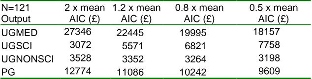
Since the size of AIC depends on the value assumed for the output vector, AICs are also estimated in Table 4B across small (50% and 80% of mean output) and large (120% and 200% of mean output) HEIs. This is done for the RE model only.

<Tables 4A and 4B here>

The results obtained from both models are broadly similar (see panel A of Table 4). The AIC of undergraduate medicine varies from £17600 per annum from the SFA model to £21000 per annum from the RE model); that associated with undergraduate science is around £6,000 a year, while undergraduate non-science has an AIC of about £3,500 per year. Meanwhile, postgraduate education has an AIC which varies from £7,500 (when estimated using SFA) to about £10,500 per year (when estimated using RE). It should be noted that the SFA method predicts cost levels that that are in general below those estimated using RE, and this is as we might expect given that SFA, unlike RE, is a frontier method.

The estimated AICs are indicative rather than definitive and should be used with some caution. There is no established method by which we can attach confidence intervals to these estimates. (It may in principle be possible to do this using bootstrapping methods, but this would be an innovation to this literature that lies beyond the scope of the present paper.) The AICs as noted above are computed by setting all outputs at prespecified values (for example mean or 120% of mean levels). The further the actual outputs at an HEI are from the levels used in the calculation the bigger the likely discrepancy in its actual AICs from those estimated in Table 4.

element; and group D refers to all other subjects. Groups A and B correspond exactly to our definitions of medicine and other science respectively, while groups C and D are combined into undergraduate non-science. The pattern of AICs in these figures corresponds with the pattern observed in the statistical estimates. This raises the question of whether the statistical cost functions are simply describing a funding formula. We would argue that this is unlikely to be the case for several reasons. First, while the pattern is the same, the level in the case of undergraduate medicine is considerably different. Second, the specification of the model includes several variables that are not formula funded – including postgraduate numbers, research, and third mission work. Indeed, it should be noted that less than 40% of universities' income comes from the funding council; other main sources of income include research grants and contracts, tuition fees (including those paid at higher rates by overseas students), and other income (often due to ‘third mission’ work). It is widely held that institutions cross-subsidise, for example from revenue gained from overseas students’ tuition fees, into other areas. All of this being so, it would appear to us to be perverse to suggest that costs mirror a formula that in any event attaches to less than half of all funding. The specification of the model is, moreover, non-linear, whereas formula funding is linear in nature. Third, the analysis is in line with other work of this kind – including work such as that of Cohn et al. (1989) which was conducted in the USA where resources are not allocated by formula. Finally, and in our view most tellingly, the use of SFA provides a safeguard against the misrepresentation of expenditures as costs since the functions estimated by SFA tell us what the parameters would be for a technically efficient institution. Nevertheless the possibility cannot be entirely dismissed that, as Bowen (1980) has argued, ‘each institution raises all the money it can’ and ‘each institution spends all it raises’.

4.2 Estimates using sub-samples

beyond the valid domain and means that the estimated AICs for these outputs in the post-1992 sector should be treated with caution.

<Table 5 here>

A further notable result is the difference between institutions in the cost of postgraduates: the AIC is around £3000 in colleges of higher education, £8000 in post-1992 HEIs and £14000 in pre-1992 universities, although the last AIC in particular should be interpreted with caution since its calculation involves extrapolation outside the valid domain. There are various possible explanations for these observed differences between groups of institutions in their estimated AICs. First, they may be a consequence of a technical problem with the model. If, owing perhaps to a paucity of observations, variation in one or more of the variables is limited, the quadratic specification can be particularly prone to problems of multicollinearity because variables appear not only in linear form but also in a multiplicity of interaction terms. Secondly, the inter-institutional difference in AICs may be a consequence of different mixes of outputs in the different groups of HEIs. Thirdly, the inter-institutional variation in the AIC of postgraduates may arise from the fact that the postgraduate output encompasses considerable variety in the type of qualifications obtained: for example, 1 year teacher training; 1 year taught masters; or 3 year doctorate. Clearly, the resources required for each type of qualification will vary and, if (as appears to be the case from the descriptive statistics in Table 2) different types of HEI specialise in different types of postgraduate qualification, this will give rise to the variation across institutions in AIC for postgraduate teaching. This is investigated further in section 4.6.

4.3 Estimates of economies of scale and scope

This section reports on measures of scale and scope economies that have been derived from the full (quadratic) specification of the model, estimated across all HEIs in the sample using both the RE and SFA estimation methods (reported in Table 3). Like AICs, these measures vary depending on the levels in the output vector used for their calculation, and so are reported for a hypothetical institution which produces average levels of all outputs identified in the model, one which produces 80% of the average level of each output, and one which produces 120% of the average level of each output. The results appear in Tables 6 and 7.

<Table 6 here> <Table 7 here>

decreasing returns with the RE model, but slightly increasing returns using SFA). Third, these broad conclusions remain the same across all sizes of institutions considered. On theoretical grounds the SFA estimates of returns to scale are to be preferred over those based on RE; economies of scale can only meaningfully be defined for efficient cost levels and the RE model estimates a cost function as a line of best fit through observations that inevitably embody some inefficiency. This may cause upward bias in both the numerator and the denominator of SR (see

Appendix section 1), and if the former bias exceeds the latter the measure of scale economies obtained by RE will exceed the true measure obtained by SFA. RE and SFA agree better on product-specific economies of scale and this in part could be because the slopes of the two functions estimated can be similar in a particular direction even if the functions are located at different levels of total cost estimated.

So far as economies of scope are concerned, there is a greater disagreement between the estimating methods than is the case for economies of scale. The RE model predicts both global and product-specific economies of scope (the former are substantial), while the SFA model predicts diseconomies of scope except in the case of undergraduate science where scope economies are observed across all sizes of institution. This is likely due to the fact that in the SFA specification there are fewer overhead costs to be allocated amongst the various outputs. These findings have implications regarding the appropriate choice of expansion policy. These are discussed further in section 4.8.

<Table 8 here>

4.4 Estimates of efficiency

to establish more conclusively what is going on – but it may be the case that specialised institutions have, for legitimate reasons, greater demands on space and other resources than do other institutions. For example, art students need studio space. Clearly further investigation into the possible determinants of cost efficiency is vital.

4.5 An augmented model

The model estimated thus far is extremely simple in that the vector of explanatory variables is made up only of the various outputs produced by HEIs. As suggested in section 2.1, a cost function might also include some measure of factor prices. Cohn et al (1989) included average annual faculty salary to reflect labour prices, but this is not a satisfactory measure of differences in academic labour costs for a number of reasons. First, the classification of staff as academic or non-academic may not be consistent across institutions. Second, in calculating average salary, an arbitrary decision needs to be made regarding what weighting to give part-time staff. Finally, even if these two problems were resolved, the resulting measure of average academic salary would reflect not just differences in labour prices faced by HEIs but also differences in the composition of their staff.

An alternative approach to allowing for differences in factor prices in the cost equation is therefore to construct a dummy for location in London where staff (and possibly capital) prices are likely to be higher than elsewhere. We have therefore estimated an equation which augments the vector of explanatory variables with a London dummy, and interactions between the London dummy and the 6 outputs (as in Cohn et al., 1989). The results, which we do not report in full for reasons of space, indicate that location in London and the additional interaction variables are insignificant in the cost equation (with the exception of the marginally significant interaction of LONDON and UGMED).

4.6 The role of quality

(first=80, upper second=65, lower second=55, third=45, unclassified=37.5). The initial result was confirmed.

4.7 Postgraduate education

The inter-institutional differences in the types of qualifications undertaken by postgraduates have been noted in Table 2. In fact, pre-1992 universities have a considerably higher percentage of postgraduates undertaking research (37%) than either post-1992 or colleges of higher education (which have 11% and 7% respectively), while post- and pre-1992 institutions have much higher percentages of taught postgraduates (at 55% and 47% respectively) than colleges of higher education (at 26%). Of the relatively small number of postgraduates in colleges of higher education, 67% are in the 'other' category which is made up of, inter alia, teacher training qualifications. In the preceding analysis lack of degrees of freedom determined that only a single measure of postgraduate activity was included on the right hand side, despite this variation.

To preserve degrees of freedom, a linear cost equation, which includes all of the outputs defined earlier but which splits postgraduates into three categories (namely research, taught and other), estimated using RE and SFA, respectively, is displayed in Table 9. The linear specification also makes the estimated coefficients easy to interpret, since these now equate to average incremental costs. The pattern of undergraduate AICs is as reported in Table 4. The AIC for postgraduate tuition, however, is between about £11,000 and £14,000, and is relatively high compared to the AICs for postgraduate research (£2500 to £3500) and other postgraduates (£3000 to £4000). The result regarding postgraduate research is, at first sight, surprising given the intensive supervision on a one-to-one basis often provided for research students. It may be the case that the gross cost associated with the provision of doctoral training is indeed low in some subject areas. More generally, though, the result may be a consequence of the fact that research postgraduates often provide input into the undergraduate teaching and research functions of the institution, thereby reducing the net costs associated with doctoral students. The low AIC of the other postgraduates category may be a consequence of the inclusion in this category of teacher training where much of the course involves practical experience in the workplace. The large percentage of postgraduates in colleges of higher education falling into this category may therefore explain the low AIC for postgraduates reported in Table 5, where costs were estimated for each subgroup of institutions separately.

4.8 Evaluating expansion policies

It is possible to use the estimated cost function to evaluate the costs of expanding higher education outputs, and, more importantly, to identify whether expansion should take place in existing institutions, or whether it would be better to provide new HEIs (although the latter policy would incur one-off building costs which have not been taken into account in the cost equations estimated in this paper). This section therefore considers a number of expansion scenarios and evaluates the costs of expansion using both the RE and SFA models. The application of the different estimating methods turns out to provide starkly different results, and the implications for policy need careful consideration. In using the RE model, the cost function is calculated as a line of 'best fit' through the data – this takes as a given the fact that HEIs are less than perfectly efficient. In applying the SFA model to this exercise, however, since the cost function is a frontier around the data, the estimates it provides of the costs of expansion will be founded on the premise that existing and new institutions are all made to be efficient. If policy-makers believe that it is possible to achieve such efficiency, then the results of the SFA analysis may provide a firm basis for policy. Otherwise, more weight should be given to the results of the RE analysis.

In all cases, the models (RE and SFA) from Table 3 are used in the expansion estimations, the Oxbridge dummy is set to zero, and the base situation is considered to be one in which there are 120 institutions each of which produces an identical output vector which is the average amount of each output. (In fact, there are 121 instutitions in our sample; the illustrative examples provided in the remainder of this section are easier to compute using 120, since 25% of 120 is an integer.) Initially, we consider the scenario in which higher education outputs are all simultaneously increased by 25%, and the cost effects will be evaluated using the RE and SFA models respectively. The RE model estimates total global current costs (that is costs of 120 HEIs producing average levels of output) to be £10008m, and if the 25% increase in output is effected by increasing output in existing HEIs, then costs rise to £12302m, a rise of 22.9%. The rise in costs from increasing the number of HEIs by 25% would, of course, be 25% (excluding the set-up costs). Thus the conclusion is that such an expansion should be achieved through increasing output in existing institutions, because of the ray economies of scale observed in the RE cost model.

introducing more 'typical' HEIs to the sector rather than by increasing the size of the existing HEIs. In order to make a definitive decision, however, the set-up costs need to be compared with the discounted annual savings in costs over the lifetime of the new HEIs.

It should be noted also that the above analysis raises by 25% the outputs of all institutions irrespective of whether, on an individual basis, the institution faces increasing, constant or decreasing economies of scale. It is possible to develop a more discerning policy so that changes are targeted in line with the nature of returns to scale faced by each individual institution. Such an approach would likely be more effective for securing savings as it would essentially move each institution to its own most productive scale size given its mix of activities and their current levels.

Consider now the scenario in which undergraduate numbers are expanded by 25% (in all subjects), but all other outputs remain at the current average level. The RE model predicts the total costs once this increase has been effected in existing institutions to be £11000m (or a 9.9% increase). This compares with £11430m (or a 12.4% increase) which are the costs when 30 additional HEIs specialising only in undergraduate teaching are introduced to the sector, each producing average levels of undergraduates (in each subject) and zero levels of other outputs. Alternatively, if 10 HEIs specialising in undergraduate medicine, 10 in undergraduate science and 10 in undergraduate non-science are introduced and set up to achieve the same increase in student numbers, total costs are estimated to be £11382m (an increase of 13.7%). The preference in the RE model is therefore to expand existing HEIs and should come as no surprise given the product-specific economies of scale and scope predicted by this cost model for undergraduates. By way of comparison, the SFA model predicts these figures to be £9685m (i.e. an 11.6% increase), £9889m (a 14.0% increase) and £9782m (a 12.7% increase), respectively, and therefore confirms the result of the RE model in this instance. Product-specific economies of scale for undergraduate science and non-science, and product-specific economies of scope for undergraduate science generate the observed result.

These results hold good so long as expansion does not entail such a diminution of intake quality that costs are markedly affected. The results on quality reported above do not suggest that this is likely to be a problem, but the planned expansion of the age-participation rate to 50% is not a marginal change, and it should be borne in mind that this increase in higher education provision may have implications for costs that cannot be modelled simply by looking at historical data as we do here.

functions. The calculations do also indicate the potential for conflicting policy implications arising from the choice of estimation method, which itself is underpinned by the analyst's assumptions about the attainability of technical efficiency both in existing and new institutions.

5. Conclusions

This paper extends the literature on higher education costs by refining the disaggregation of subjects, introducing third mission activities into the model, examining the cost differentials between different types of postgraduate qualification, considering the role played by location, and evaluating the importance of differentials in the quality of both student intake and output. The analysis also allows some simple examination of the cost implications of different expansion policies, and of the efficiency differentials that exist between institutions. This is all done using panel data drawn from the early years of the present decade for a sample of English institutions of higher education.

Amongst undergraduates, medical students are found to be the most costly, and non-science students the least. Amongst postgraduates, those on taught courses are costly, while research students (presumably because they provide a source of cheap teaching and research assistance) are relatively inexpensive. This last finding contrasts spectacularly with the results obtained by HEFCE’s cost transparency exercise (probably because the latter calculates the gross costs of research students rather than, as here, the net costs). Location in London and quality considerations do not appear to impact significantly on the analysis.

Estimates of economies of scale and economies of scope vary according to the choice of estimating technique. The RE model suggests that ray economies of scale and economies of scope are ubiquitous (though generally not huge). The SFA model suggests some product-specific economies of scale in research, but diseconomies elsewhere, and product product-specific economies of scope in undergraduate science, but diseconomies elsewhere. As a consequence, the RE model predicts that uniform expansion of all outputs can most efficiently be realised by expansion of the existing institutions rather than by creation of new ones, whereas the SFA model predicts that such an expansion should be effected by creating new (efficient) HEIs so long as the one-off set-up costs are less than the discounted savings in annual costs achieved over the lifetime of the new HEIs. When, however, an unbalanced expansion of outputs is considered (that is expansion only of undergraduates), both estimating techniques indicate that such an expansion is best achieved by expanding existing HEIs than by creating new institutions specialising in undergraduate provision.

Table 1: Definition of variables used in the analysis

Variable Description

COSTDEF (Dependent variable) Total operating costs in £000 in constant prices. This figure is inclusive of depreciation.

UGMED Full-time-equivalent (FTE) undergraduates in medicine or dentistry (000).

UGSCI FTE Undergraduate in science (000). Summation

of subjects allied to medicine, veterinary,

biological, agriculture, physical sciences, Maths, computing, engineering and architecture.

(Includes weighted average of combined category)

UGNONSCI FTE Undergraduate in non-science subjects (000). Summation of social economics, law, business, librarianship, languages, humanities, creative arts and education. (Includes weighted average of combined)

UG Total of UGMED, UGSCI and UGNONSCI

(000)

RESEARCH Quality related funding and research grants, in £000000, constant prices.

PG FTE postgraduate student numbers in 000s (NB

PG is the sum of PGR, PGT and PGOTHER).

PGR FTE postgraduate student numbers on research

programmes (000).

PGT FTE postgraduate student numbers on taught

courses (000).

PGOTHER FTE postgraduate student numbers on other postgraduate courses (000).

3RD MISSION Income from other services rendered in £m in constant prices. The ‘other services’ category of income includes all income in respect of services rendered to outside bodies, for example industrial and commercial companies and public

corportations.

Table 2: Descriptive statistics for the variables in the data set V a r i a b l e 1 M e a n S t d . D e v . M i n M a x A l l H E I s C O S T D E F 8 5 9 3 0 . 7 6 8 9 9 3 4 . 2 8 1 4 2 2 . 1 9 4 6 2 5 3 0 . 0 0 U G 6 . 1 4 8 4 . 7 5 0

0 2

0 . 1 4 9 U G M E D 0 . 2 0 7 0 . 5 4 4

0 2

. 7 2 4 U G S C I 2 . 5 5 2 2 . 2 4 3

0 7

. 7 1 9 U G N O N S C I 3 . 3 8 8 2 . 6 1 5

0 1

2 . 6 1 6 P G 1 . 7 3 3 1 . 4 4 7

0 6

. 0 6 8 P G R 0 . 4 0 . 6

0 4

5 1 8 3 5 6 P G T 0 . 8 2 9 0 . 7 2 7

0 3

. 1 2 0 P G O T H E R 0 . 4 5 3 0 . 4 5 4

0 2

. 3 4 6 R E S E A R C H 2 2 . 1 2 7 4 3 . 4 4 5

0 2

1 9 . 9 7 4 3 R D M I S S I O N 4 . 3 5 4 5 . 3 8 0

0 3

C o l l e g e s o f h i g h e r e d u c a t i o n C O S T D E F 1 7 6 3 9 . 3 6 1 2 9 7 4 . 0 1 1 4 2 2 . 1 9 5 1 0 4 6 . 4 8 U G 2 . 2 6 6 1 . 8 4 5 0 . 0 2 6 7 . 1 9 2 U G M E D

0 0 0 0

U G S C I 0 . 5 3 9 0 . 6 4 3

0 2

. 3 1 0 U G N O N S C I 1 . 7 2 6 1 . 3 7 1

0 5

. 6 2 1 P G 0 . 4 0 . 5

0 2

4 1 1 4 2 9 P G R 0 . 0 3 1 0 . 0 3 7

0 0

. 1 5 4 P G T 0 . 1 1 5 0 . 1 2 5

0 0

. 5 9 4 P G O T H E R 0 . 2 9 5 0 . 4 1 2

0 1

. 9 4 8 R E S E A R C H 0 . 4 4 5 0 . 5 7 1

0 2

. 4 6 8 3 R D M I S S I O N 0 . 7 1 5 1 . 5 3 7

0 8

5 9 0 0 0 U G 1 0 . 3 4 2 3 . 1 5 5 4 . 6 6 9 1 9 . 7 5 3 U G M E D

0 0 0 0

U G S C I 4 . 3 7 1 1 . 4 6 8 1 . 1 6 3 7 . 4 6 4 N O N S C I 5 . 9 7 1 2 . 1 6 9 2 . 5 9 0 1 2 . 6 1 6 P G 2 . 1 3 2 0 . 8 6 6 0 . 7 6 8 4 . 0 7 8 P G R 0 . 2 3 3 0 . 1 2 7

0 0

S S I O N 0 T r a d i t i o n a l ( p r e -1 9 9 2 ) H E I s C O S T D E F 1 3 5 9 6 0 . 9 3 1 1 4 4 7 3 . 6 3 9 6 1 6 . 4 0 4 6 2 5 3 0 . 0 0 U G 6 . 3 3 2 4 . 7 3 5

0 2

0 . 1 4 9 U G M E D 0 . 5 0 2 0 . 7 5 5

0 2

. 7 2 4 U G S C I 2 . 8 8 2 2 . 2 5 5

0 7

. 7 1 9 N O 2 . 2 .

0 1

N S C I 9 4 7 3 1 4 . 2 2 3 P G 2 . 4 5 2 1 . 5 7 7 0 . 1 1 0 6 . 0 6 7 P G R 0 . 9 1 5 0 . 8 6 0

0 4

. 5 5 6 P G T 1 . 1 5 0 0 . 7 3 1

0 3

. 1 2 1 P G O T H E R 0 . 3 8 8 0 . 3 6 4

0 1

. 6 1 3 R E S E A R C H 5 0 . 0 3 3 5 6 . 8 8 9 0 . 3 1 9 2 1 9 . 9 7 4 3 R D M I S S I O N 6 . 7 9 5 6 . 9 3 3

0 3

1 . 0 4 2

Table 3: Estimated coefficients of the quadratic cost function

Variables1

Random effects Coefficients

(z value)

Stochastic frontier Coefficients

(z value)

UGMED 15094.60 14477.65

(1.80) (1.28)

UGSCI 9320.50 9500.10

(5.50) (4.34)

UGNONSCI 3088.18 3879.17

(2.88) (2.36)

PG 8553.31 4822.26

(3.03) (1.45)

RESEARCH 921.02 986.07

(6.67) (4.57)

3RD MISSION 1154.03 1021.76

(6.13) (10.13)

UGMED X UGSCI 3135.91 1893.80

(1.65) (0.66)

UGMEDX UGNSCI 6110.62 6181.28

(3.66) (2.06)

UGMED X PG -16723.98 -17192.70

(6.68) (3.10)

UGMED X RES 294.60 310.15

(3.11) (1.29)

UGSCI X UGNSCI -341.05 -276.31

(0.84) (0.34)

UGSCI X PG -1233.85 -1221.13

(1.77) (1.12)

UGSCI X RES -24.97 -19.51

(0.87) (0.36)

UGNSCI X PG 898.74 801.92

(1.73) (0.92)

UGNSCI X RES -85.68 -83.43

(3.74) (1.44)

PG X RES 257.01 253.21

(7.13) (2.31)

UGMEDSQ -582.49 1340.00

(0.14) (0.26)

UGSCISQ 27.87 -16.03

(0.09) (0.02)

UGNONSCISQ 47.38 -22.25

(0.26) (0.07)

PGSQ -0.58 644.56

(0.00) (.51)

RESSQ -2.86 -3.11

(3.45) (1.08)

OXBRIDGE 57581.42 45107.88

(3.49) (1.44)

Constant 6299.86 -2679.10

(3.07) (0.95)

Lagrangian test for random effects chi2=183.78

Log likelihood function -3704.98

n 121x3 121x3

Table 4A: AICs calculated the two quadratic models at the mean levels of output (full sample)

N=121 Output

Random effects AIC (£)

Stochastic frontier AIC (£)

UGMED 21220 17603

UGSCI 6196 6368

UGNONSCI 3308 3925

PG 10664 7574

Table 4B: AICs calculated using RE at 1.2 times and 0.8 times the mean levels of output (full sample)

N=121 Output

2 x mean AIC (£)

1.2 x mean AIC (£)

0.8 x mean AIC (£)

0.5 x mean AIC (£)

UGMED 27346 22445 19995 18157

UGSCI 3072 5571 6821 7758

UGNONSCI 3528 3352 3264 3198

PG 12774 11086 10242 9609

Table 5: Average incremental costs across subgroups calculated at mean output level using a quadratic specification

SCOPs n = 38

Post-1992 HEIs n = 33

Traditional(pre-1992) HEIs n = 50

RE

UGMED 20449

UGSCI 8241 2581 8448

UGNONSCI 3180 2890 3581

PG 2788 7725 13914

Table 6: Economies of scale (all HEIs)

a) Based on the RE model shown in column 1 of Table 31

Evaluated at:

Mean2 80% of mean 120% of mean

Ray economies 1.09 1.11 1.08

Product-specific economies

Medicine Ug 1.01 1.00 1.01

Science Ug 0.99 0.99 0.98

Non-science Ug 0.95 0.96 0.95

Postgraduate 1.00 1.00 1.00

Research 1.07 1.05 1.08

b) Based on the SFA model shown in column 2 of Table 31

Evaluated at:

Mean2 80% of mean 120% of mean

Ray economies 0.96 0.96 0.97

Product-specific economies

Medicine Ug 0.98 0.99 0.98

Science Ug 1.01 1.00 1.01

Non-science Ug 1.02 1.02 1.02

Postgraduate 0.87 0.89 0.86

Research 1.07 1.05 1.08

1. Oxbridge is set to zero.

2. Mean is the arithmetic mean over the 3 years (i.e. 363 observations).

Table 7: Economies of scope (all HEIs)

a) Based on the RE model shown in column 1 of Table 31 Evaluated at:

Mean2 80% of mean 120% of mean

Global economies 0.38 0.46 0.32

Product-specific economies

Medicine Ug 0.06 0.08 0.04

Science Ug 0.17 0.17 0.18

Non-science Ug 0.07 0.09 0.06

Postgraduate 0.03 0.06 0.01

Research 0.04 0.06 0.01

Other services 0.08 0.09 0.06

b) Based on the SFA model shown in column 2 of Table 31 Evaluated at:

Mean2 80% of mean 120% of mean

Global economies -0.18 -0.23 -0.15

Product-specific economies

Medicine Ug -0.05 -0.05 -0.04

Science Ug 0.07 0.04 0.10

Non-science Ug -0.04 -0.05 -0.04

Postgraduate -0.08 -0.08 -0.08

Research -0.09 -0.09 -0.09

Other services -0.04 -0.05 -0.03

1. Oxbridge is set to zero.

Table 8: Descriptive statistics for the efficiency estimates from the stochastic frontier analysis (2002/03)

n mean standard deviation

All HEIss 121 0.69 0.32 post-1992 HEIs 33 0.84 0.077 pre-1992 HEIs 50 0.80 0.23 Colleges of higher

education

Table 9: Undergraduate and postgraduate activity disaggregated, RE estimation

Variable1 RE

coefficient (z value)

SFA coefficient (z value)

UGMED 17102.04 17133.67

(5.32) (5.36)

UGSCI 5232.08 4976.06

(8.27) (11.28)

UGNONSCI 4408.90 4630.67

(8.42) (10.08)

PGR 3641.65 2517.67

(1.08) (0.93)

PGT 13887.25 10822.43

(9.17) (8.42)

PGOTH 3045.69 4258.06

(1.49) (1.44)

RESEARCH 1226.68 1209.07

(20.93) (28.98) 3RD MISSION 1228.21 1114.39

(6.37) (1.49)

OXBRIDGE 59504.42 64322.27

(4.92) (3.48)

CONS 6076.04 -2941.36

(3.90) (1.37)

log likelihood -3750.65

n 121x3 121x3

1. See Table 1 for precise definitions of variables.

References

Aigner, D. and Chu, S-F. (1968) On estimating the industry production function, American Economic Review, 58, 826-839.

Battese, G.E. and Coelli, T.J. (1995), A model for technical inefficiency effects in a stochastic frontier production function for panel data, Empirical Economics, 20, 325-332.

Baumol, W.J., Panzar, J.C. and Willig, R.D. (1982) Contestable markets and the theory of industry structure, San Diego: Harcourt Brace Jovanovich.

Bowen, H.R. (1980) The costs of higher education, San Francisco: Jossey Bass.

Breusch, T.S. and Pagan, A.R. (1980) The Lagrange Multiplier test and its applications to model specifications in econometrics, Review of Economics Studies, 47, 239-253.

Cohn, E., Rhine, S. & Santos, M. (1989) Institutions of higher education as multi-product firms: economies of scale and scope Review of Economics and Statistics, 71, 284-290.

Cohn, E. & Cooper, S.T.(2004) Mulitproduct cost functions for universities: economies of scale and scope in Johnes, G & Johnes, J (eds) The International Handbook on the Economics of Education, Edward Elgar, Cheltenham.

Glass, J.C., McKillop, D.G. & Hyndman (1995a) Efficiency in the provision of university teaching and research: an empirical analysis of UK universities Journal of Applied Econometrics, 10, 61-72.

Glass, J.C., McKillop, D.G. and Hyndman (1995b) The achievement of scale efficiency in UK universities: a multiple-input multiple-output analysis Education Economics, 3, 249-263.

Greene, W. (2002) Fixed and random effects in stochastic frontier models, mimeo available at http://pages.stern.nyu.edu/~wgreene/fixedandrandomeffects.pdf.

Izadi, H., Johnes, G., Oskrochi, R. and Crouchley, R. (2002) Stochastic frontier estimation of a CES cost function: the case of higher education in Britain Economics of Education Review, 21, 63-71.

Johnes, G. (1996) Multi-product cost functions and the funding of tuition in UK universities Applied Economics Letters, 3, 557-561.

Johnes, G. (1997) Costs and industrial structure in contemporary British higher education Economic Journal, 107, 727-737.

Johnes, G. (1998a) The costs of multi-product organization and the heuristic evaluation of industrial structure Socio-Economic Planning Sciences, 32, 199-209.

Johnes, G (1999) 'The management of universities: Scottish Economic Society / Royal Bank of Scotland Annual Lecture', Scottish Journal of Political Economy, 46 pp505-522.

Johnes, G. (2004) A fourth desideratum: the CES cost function and the sustainable configuration of multiproduct firms, Bulletin of Economic Research, 56, 329-332.

Johnes, G., Johnes, J., Thanassoulis, E., Lenton, P. and Emrouznejad, A. (2005) An exploratory analysis of the costs of higher education in England, Nottingham: Department for Education and Skills.

Jondrow, J., Lovell, C.A.K., Materov, I.S. and Schmidt, P. (1982) On the estimation fo technical inefficiency in the stochastic frontier production function model, Journal of Econometrics, 19, 233-238.

Nerlove, M. (1971) A note on error components models, Econometrica, 39, 383-396.

Scheffe, H. (1956) Alternative models for the analysis of variance, Annals of Mathematical Statistics, 27, 251-271. Stevens, P.A. (2005) A stochastic frontier analysis of English and Welsh Universities, Education Economics, 13(4)

forthcoming.

Verry, D.W. and Layard, P.R.G. (1975) Cost functions for university teaching and research Economic Journal, 85, 55-74.

Appendix: Returns to Scale and Returns to Scope

1. Ray returns to scale

Ray economies (or diseconomies) of scale are defined in the multi-product case as the cost savings (or dissavings) arising when the size of the aggregate output expands but the composition of output (that is, the output mix) remains constant. The extent of the ray economies of scale (SR) that are observed may be calculated in the general case as:

∑

i i i R

y C y

y C S

) ( ) (

where C(y) is the cost of producing the output vector y and Ci(y) is the marginal cost of

producing the ith output so that C_i(y)=∂C(y)/∂y_i =MC_i. If SR > 1 (SR < 1) then there are said

to be ray economies of scale (diseconomies of scale).

2. Product-specific returns to scale

Product-specific economies (or diseconomies) of scale are the cost savings (or dissavings) which occur when the level of one product increases while the levels of the rest of the outputs remain fixed. The incremental cost of producing output i (IC(y_i)) is defined as:

) ( ) ( )

(y_i C y_n C y_{n i}

IC = − ₋

where C(y_n)is the total cost of producing all the outputs at the levels in yn, while C(y_n−_i)is the

total cost of producing all the outputs at the levels in yn except output i which is held at zero. The

average incremental cost of product i is then defined in the general case as:

[

]

i C y C y y IC y y

y

AIC( )= ( )− ( ₋ ) = ( )

If the average incremental cost of product i exceeds its marginal cost then we have product-specific returns to scale for product i. Thus, product-product-specific returns to scale for product i

(S_i(y)) are:

) ( ) ( )

(y AIC y C y

S_i = _{i i}

If S_i(y)>1 (S_i(y)<1) then there are product-specific economies (diseconomies) of scale for product i.

3. Global returns to scope

∑

i i

y C y

C( ) ( )

we have global economies of scope. The degree of global economies of scope is measured by

G

S where

( ) ( )

( )

S

i i G

    

  

−

=

∑

If S_G >0(< 0) then global economies (diseconomies) of scope exist for producing the outputs jointly rather than in separate firms.

4. Product-specific returns to scope

A measure of product-specific economies of scope (SC_i) is given by:

[

]